Sublinear Regret for Learning POMDPs
Abstract
We study the model-based undiscounted reinforcement learning for partially observable Markov decision processes (POMDPs). We propose a learning algorithm for this problem, building on spectral method-of-moments estimations for hidden Markov models, the belief error control in POMDPs and upper-confidence-bound methods for online learning. We establish a regret bound of for the proposed learning algorithm where is the learning horizon. This is, to the best of our knowledge, the first algorithm achieving sublinear regret for learning general POMDPs.
keywords
Partially Observable MDP, Online Learning, Exploration-Exploitation, Spectral Estimator1 Introduction
The partially observable Markov decision process (POMDP) is a framework for dynamic decision-making when some evolving state of the system cannot be observed. It extends the Markov decision process (MDP) and can be used to model a wide variety of real-world problems, ranging from healthcare to business. The solution to POMDPs is usually through a reduction to MDPs, whose state is the belief (a probability distribution) of the unobserved state of the POMDP, see e.g. Krishnamurthy 2016 for an overview.
We study the problem of decision making when the environment of the POMDP, such as the transition probability of the hidden state and the probability distribution governing the observation, is unknown to the agent. Thus, the agent has to simultaneously learn the model parameters (we use “environment” and “parameters” interchangeably) and take optimal actions. Such online learning framework has received considerable attention in the last decades (Sutton and Barto 2018). Despite the practical relevance of POMDPs, the learning of POMDPs is considered much more challenging than finite-state MDPs and few theoretical results are known. This is not surprising: even with a known environment, the corresponding belief MDP features a continuous state space. When the environment is unknown, we face the additional difficulty of not being able to calculate the belief accurately, whose updating formula is based on the environment. This is in contrast to the learning of standard MDPs, in which the state is always observed exactly.
To tackle this daunting task, we provide an algorithm that achieves sublinear regret, which is a popular measure for the performance of a learning algorithm relative to that of the oracle, i.e., the optimal policy in the known environment. This is the first algorithm that achieves sublinear regret, to our knowledge, in the general POMDP setup we consider. We summarize the three major contributions of this paper below.
In terms of problem formulation, we benchmark our algorithm against an oracle and measure the performance by calculating the regret. The oracle we consider is the strongest among the recent literature (Azizzadenesheli et al. 2016, Fiez et al. 2018). In particular, the oracle is the optimal policy of the POMDP with a known environment in terms of the average reward over an infinite horizon. Such an oracle has higher average reward than the oracles that use the best fixed action (Fiez et al. 2018) or the optimal memoryless policy (the action only depends on the current observation) (Azizzadenesheli et al. 2016). Still our algorithm is able to attain sublinear regret in the length of the learning horizon. This implies that as the learning horizon increases, the algorithm tends to approximate the strong oracle more accurately.
In terms of the algorithmic design, the learning algorithm we propose (see Algorithm 1) has two key ingredients. First, it builds on the recent advance on the estimation of the parameters of hidden Markov models (HMMs) using spectral method-of-moments methods, which involve the spectral decomposition of certain low-order multivariate moments computed from the data (Anandkumar et al. 2012, Anandkumar et al. 2014, Azizzadenesheli et al. 2016). It benefits from the theoretical finite-sample bound of spectral estimators, while the finite-sample guarantees of other alternatives such as maximum likelihood estimators remain an open problem (Lehéricy 2019).1. 1. endnote: 1. There are recent advances on the EM algorithm that are applied to likelihood-based methods for HMMs (balakrishnan2017statistical, yang2017statistical) with finite-sample analysis. However, the conditions on the function and the resulting basin of attraction are hard to translate to our setting explicitly. Second, it builds on the well-known “upper confidence bound” (UCB) method in reinforcement learning (Auer and Ortner 2006, Jaksch et al. 2010). We divide the horizon into nested exploration and exploitation phases. We use spectral estimators in the exploration phase to estimate the unknown parameters such as the transition matrix of the hidden state, which itself is a function of the action in the period. We apply the UCB method to control the regret in the exploitation phase based on the estimated parameters in the exploration phase and the associated confidence regions. Although the two components have been studied separately before, it is a unique challenge to combine them in our setting. In particular, the belief of the hidden state is subject to the estimation error. We re-calibrate the belief at the beginning of each exploitation phase based on the most recent estimate of the parameters. This helps us achieve the sublinear regret.
In terms of regret analysis, we establish a regret bound of for our proposed learning algorithm where is the learning horizon. Our regret analysis draws inspirations from Jaksch et al. 2010, Ortner and Ryabko 2012 for learning MDPs and undiscounted reinforcement learning problems, but the analysis differs significantly from theirs since there are two main technical challenges in our problem.
First, the belief in POMDPs, unlike the state in MDPs, is not directly observed and needs to be estimated. This is in stark contrast to learning MDPs (Jaksch et al. 2010, Ortner and Ryabko 2012) with observed states. As a result, we need to bound the estimation error of the belief which itself depends on the estimation error of the model parameters. In addition, we also need to bound the error in the belief transition kernel, which depends on the model parameters in a complex way via Bayesian updating. To control these errors, we extend the approach in De Castro et al. 2017 for HMM to POMDP, and relate the error in belief transitions to the estimation error of POMDP parameters and the belief state error.
Second, to establish the regret bound, we need an uniform bound for the span of the bias function (also referred as the relative value function) for the optimistic belief MDPs which have continuous state spaces. Such a bound is often critical in the regret analysis of undiscounted reinforcement learning of continuous MDP, but it is often shown under restrictive assumptions such as the Hölder continuity that do not hold for the belief state in our setting (Ortner and Ryabko 2012, Lakshmanan et al. 2015). We develop a novel approach to bound the bias span for the undiscounted POMDP by bounding the Lipschitz modulus of the optimal value function for infinite-horizon discounted problems when the discount factor tends to one. One key step is to bound the Lipschitz module of the belief transition kernels using the Kantorovich metric. Exploiting the connection with the infinite-horizon undiscounted problem via the vanishing discount factor method then yields an explicit bound on the bias span for the optimisitic belief MDPs.
1.1 Related Literature
This paper extends the online learning framework popularized by multi-armed bandits to POMDPs. There is a large stream of literature on the topic of bandits, see e.g. Bubeck and Cesa-Bianchi 2012 for a survey. In POMDPs, the rewards across periods are not independent any more. A stream of literature studies nonstationary/switching MAB, including Auer et al. 2002b, Garivier and Moulines 2011, Besbes et al. 2014, Keskin and Zeevi 2017, Cheung et al. 2022, Auer et al. 2019. The reward can change over periods subject to a number of switches or certain changing budget (the total magnitude of reward changes over the horizon), and the oracle is the best action in each period. It should be noted that the oracle considered is stronger than ours. However, all the designed algorithms in this literature require finite switches or sublinear changing budget (in the order of ). This is understandable, as there is no hope to learn such a strong oracle if the actions can be completely different across periods. In our setting, the number of changes (state transitions) is linear in and the algorithms are expected to fail to achieve sublinear regret even measured against our oracle, which is weaker than the oracle in this stream of literature. There are a few exceptions, including Zhu and Zheng 2020, Chen et al. 2021, Zhou et al. 2021, which study models with linear changing budget but specific structures. In Chen et al. 2021, the rewards are cyclic which can be leveraged to learn across cycles despite of the linear change. In Zhu and Zheng 2020, the reward grows over time according to a function. In Zhou et al. 2021, the reward is modulated by an unobserved Markov chain. Another stream of literature investigates the so-called restless Markov bandit problem, in which the state of each action evolves according to independent Markov chains, whose states may not be observable. See, for example, Slivkins and Upfal 2008, Guha et al. 2010, Ortner et al. 2014. The POMDP model we consider has a more complex structure. Thus the algorithms proposed in the above studies cannot achieve sublinear regret.
Our work is related to the rich literature on learning MDPs. Jaksch et al. 2010 propose the UCRL2 (Upper Confidence Reinforcement Learning) algorithm to learn finite-state MDPs and prove that the algorithm can achieve the optimal rate of regret measured against the optimal policy in terms of the undiscounted average reward. Follow-up papers have investigated various extensions to Jaksch et al. 2010, including posterior sampling (Agrawal and Jia 2017), minimax optimal regret (Azar et al. 2017, Zhang and Ji 2019), and the model-free setting (Jin et al. 2018). Cheung et al. 2019 consider the case where the parameters of the MDP, such as the transition matrix, may change over time. The algorithms are not applicable to our setting, because of the unobserved state in POMDPs. However, since a POMDP can be transformed to a continuous-state MDP, our setting is related to the literature, especially those papers studying MDPs with a continuous state space. Ortner and Ryabko 2012, Lakshmanan et al. 2015 extend the algorithm in Jaksch et al. 2010 to a continuous state space. Still, our problem is not equivalent to the learning of continuous-state MDPs. First, in this literature Hölder continuity is typically assumed for the rewards and transition probabilities with respect to the state, in order to aggregate the state and reduce it to the discrete case. However, this assumption does not hold in general for the belief state of POMDPs, whose transition probabilities are not given but arise from the Bayesian updating. Second, even if the continuity holds, the state of the belief MDP in our problem, which is the belief of the hidden state, cannot be observed. It can only be inferred using the estimated parameters. This distinguishes our problem from those studied in this literature. The algorithm and analysis also deviate substantially as a result. There are studies that focus on the applications such as inventory management (Zhang et al. 2018, Chen et al. 2019, Zhang et al. 2020, Chen et al. 2020, Nambiar et al. 2021) and handle specific issues such as demand censoring and lost sales.
Our work is related to studies on reinforcement learning for POMDPs, see e.g. Ross et al. 2011, Spaan 2012 and references therein. Guo et al. 2016 propose a learning algorithm for a class of episodic POMDPs, where the performance metric is the sample complexity, i.e. the time required to find an approximately optimal policy. Recently, Jin et al. 2020 give a sample efficient learning algorithm for episodic finite undercomplete POMDPs, where the number of observations is larger than the number of hidden states. Their focus is on the sample complexity, while the method may potentially be used in the regret analysis of our infinite-horizon average reward setting. There is also a growing body of literature that apply deep reinforcement learning methods to POMDPs, see e.g. Hausknecht and Stone 2015, Igl et al. 2018. Our work differs from these papers in that we study the learning of ergodic POMDPs in an unknown environment and we focus on developing an learning algorithm with sublinear regret guarantees. A concurrent study (Kwon et al. 2021) considers regret minimization for reinforcement learning in a special class of POMDPs called latent MDP. The hidden state is static in their work while it is dynamic in our setting.
Furthermore, our work is related to the literature on the spectral method to estimate HMMs and its application to POMDPs. For instance, Anandkumar et al. 2012, Anandkumar et al. 2014 use the spectral method to estimate the unknown parameters in HMMs, by constructing the so-called multi-views from the observations. The spectral method is not readily applicable to POMDPs, because of the dependence introduced from the actions. Azizzadenesheli et al. 2016 address the issue by restricting to memoryless policies, i.e., the action only depends on the observation in the current period instead of the belief state. They extend the spectral estimator to the data generated from an arbitrary distribution other than the stationary distribution of the Markov chain, which is necessary in learning problems when the policy needs to be experimented.
There are two papers whose methodology is closely connected to this paper that warrant more discussion (Azizzadenesheli et al. 2016, De Castro et al. 2017). Azizzadenesheli et al. 2016 use spectral estimators and upper confidence methods to learn POMDPs and establish a regret bound of . One main difference between our work and theirs is the choice of the oracle/benchmark. Specifically, their oracle is the optimal memoryless policy, i.e., a policy that only depends on the current reward observation instead of using all historical observations to form the belief of the underlying state. For general POMDPs, memoryless policies are suboptimal and the performance gap is linear in between their oracle and ours. Technically, it allows them to circumvent the introduction of the belief state entirely. In our setting, we need to design a new learning algorithm to achieve sublinear regret with our stronger oracle and analyze the regret. By considering the belief-based policies, several new difficulties arise in our setting. First, the spectral method can not be applied to samples generated from belief-based policies due to history dependency; Second, the belief states can not be observed and need to be calculated using the estimated parameters, which is not an issue in Azizzadenesheli et al. 2016 because the observation in the current period can be regarded as the state. We tackle these difficulties by using an exploration-exploitation interleaving approach in the algorithm design. In particular, we develop three recipes to analyze the regret. First, we develop a novel approach to upper bound the span of the bias function for the average-reward POMDP model. In general the bias span is a complicated function of the POMDP model parameters. Our paper appears to be the first to make the bound explicit in terms of the smallest element of the transition matrices, and this is one of our main methodological contributions. This result is significant as it simultaneously provides bounds on the bias span of the estimated POMDP and the optimistic POMDP when they are close to the true POMDP model in terms of model parameters. Our bound on the bias span is different from the diameter of the POMDP discussed in Azizzadenesheli et al. 2016. The diameter in Azizzadenesheli et al. 2016 is only for observation-based policies, not for belief-state based policies we consider. Second, to control the regret, we bound the error in the belief state incurred by the errors in the estimation of POMDP parameters. We extend the approach in De Castro et al. 2017, which study filtering and smoothing errors in the context of nonparametric hidden Markov models. Such HMM models do not involve actions or decision making as in the POMDP model we consider. Third, to control the regret, we also bound the error in the (estimated) belief transition law. This is similar to online learning of finite-state MDPs where one often bounds the error in the estimates of transition probabilities in model-based methods. However, our problem is more sophisticated because the belief state is not observed, and hence can not be directly estimated. Therefore, we control this error in the transition law of beliefs by relating it to the estimation error of POMDP parameters and the belief state error.
The rest of the paper is organized as follows. In Section 2 we discuss the problem formulation. Section 3 presents our learning algorithm. In Section 4, we state our main results on the regret bounds for the learning algorithm. In Section 5, we present numerical experiments. Finally, we conclude in Section 6. All the proofs of the results in the paper are deferred to the appendix.
2 Problem Formulation
We first introduce the notation for the POMDP. A POMDP model with horizon consists of the tuple
| (1) |
where
- •
denotes the state space of the hidden state. We use to denote the state at time .
- •
denotes the action space with representing the action chosen by the agent at time .
- •
is a finite set of possible observations and denotes the observation at time .
- •
describes a family of transition probability matrices, where is the transition probability matrix for states in after the agent takes action . That is, for .
- •
The observation density function is a distribution over observations that occur in state after the agent takes action in the last period, i.e., .
- •
The reward function specifies the immediate reward for each state-action pair , and we assume the reward function for some constant
The following sequence of events occur in order in each period. In period , the underlying state transits to . Then the agent observes , whose distribution depends on and . The agent then chooses an action and receives reward determined by reward function which depends on the state and the action . Then the time proceeds to and the state transits to , whose transition probability depends on the action .
In the POMDP model, the agent does not observe the state , but only the noisy observation , after which an action is chosen. Moreover, since the agent does not know the state at time , it does not know the reward . Hence, it is typical to assume that the action does not depend on the reward in the literature (Krishnamurthy 2016, Cao and Guo 2007). Therefore, the action taken in period , , depends on the history up to time , denoted by
| (2) | ||||
| (3) |
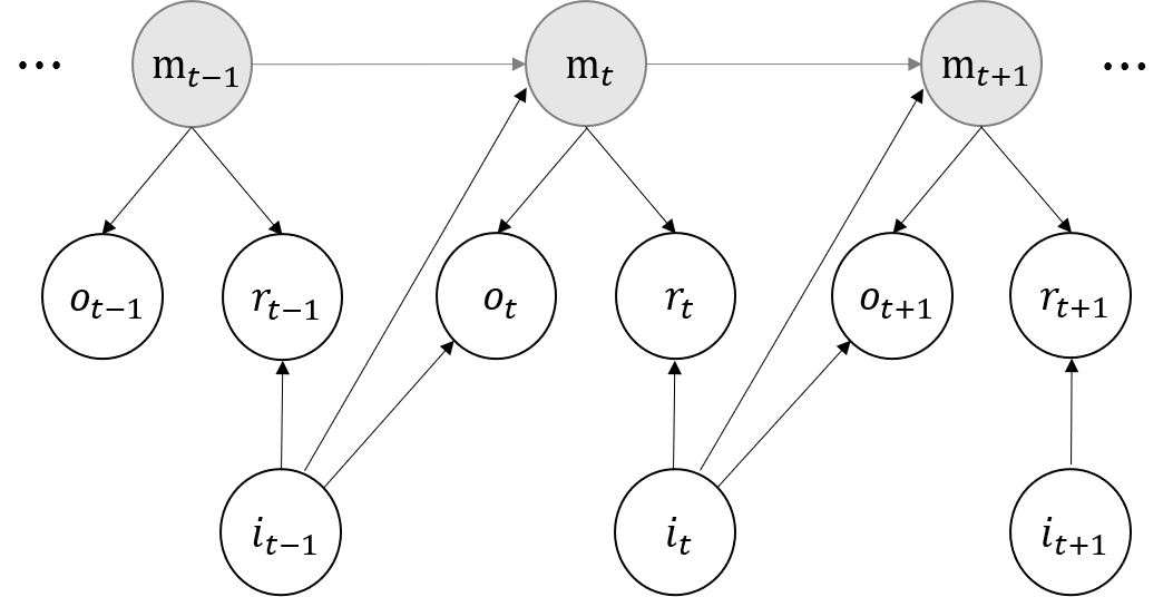
The agent attempts to optimize the expected cumulative reward over a finite horizon . The information structure is illustrated by the graph in Figure 1.
2.1 Reformulate POMDP as Belief MDP
If the model environment in (1) is known to the agent, then it is well-known (see, e.g., Krishnamurthy 2016) that to maximize the expected reward, the agent can reformulate the POMDP as an MDP with a continuous state space. The state of the MDP reflects the belief, or the distribution, over the hidden states, and thus it is referred to as the belief MDP. More precisely, define an -dimensional vector as the belief of the underlying state in period :
| (4) | ||||
Because of the Markovian structure of the belief, we can show (see, e.g., Krishnamurthy 2016, Puterman 2014) that the belief in period can be updated based on the current belief , the chosen action and the observation . In particular, the updating function determines
| (5) |
We may omit the dependence on and if it doesn’t cause confusion. By Bayes’s theorem, we have
| (6) |
where is the distribution of the observation under belief and action .
We next introduce some notations to facilitate the discussion and analysis. Define the expected reward conditional on the belief and action
| (7) |
We can also define the transition kernel of the belief conditional on the action:
| (8) |
A policy for the belief MDP is a mapping from the belief states to actions, i.e., the action chosen by the agent at time is . Following the literature (see, e.g., Agrawal and Jia 2017), we define the gain of a policy and the optimal gain.
Definition 2.1
The gain of a policy given the initial belief state , is defined as the long-run average reward for the belief MDP over an infinite horizon, given by:
| (9) |
where the expectation is taken with respect to the interaction sequence when policy interacts with the belief MDP. The optimal gain is defined by
| (10) |
2.2 Assumptions
Next we provide the technical assumptions for the analysis.
The entries of all transition matrices are bounded away from zero .
.
Assumptions 2.2 and 2.2 can be strong in general, but they are required by the state-of-art method to bound the belief error caused by the parameter miscalibration (see De Castro et al. 2017 for the HMM setting), which is essential in learning POMDPs. Moreover, the two assumptions provide sufficient conditions to guarantee the existence of the solution to the Bellman optimality equation of the belief MDP and the boundedness of the bias span; See Propositions 2.2 and 4.1. Note that Assumption 2.2 itself implies that for any fixed , the Markov chain with transition matrix is geometrically ergodic with a unique stationary distribution denoted by , and the geometric rate is upper bounded by . See e.g. Theorems 2.7.2 and 2.7.4 in Krishnamurthy 2016. This geometric ergodicity, which can hold under weaker assumptions, is needed for spectral estimations of the POMDP model as in Azizzadenesheli et al. 2016.
For each , the transition matrix is invertible.
For all , are linearly independent.
Assumption 2.2 and 2.2 are required for the finite-sample guarantee of spectral estimators (Anandkumar et al. 2012, Anandkumar et al. 2014). See Section 3.1 for more details. Since our learning algorithm uses the spectral estimator to estimate hidden Markov models, our approach inherits the assumptions.
Before we proceed, we first state a result on the characterization of the optimal gain given in Definition 2.1 and the existence of stationary optimal policies for the belief MDP (9) under the average reward criterion. Note that in general (without the assumptions), there is no guarantee that a stationary optimal policy would exist for problem (9) (see e.g. Yu and Bertsekas 2004).
Proposition 2.2
Suppose Assumptions 2.2 and 2.2 hold. There exists a bounded function and a constant such that the Bellman optimality equation holds for problem (10):
| (11) |
Moreover, there exists a stationary deterministic optimal policy for problem (10), which prescribes an action that maximizes the right side of (11). The constant is the optimal gain defined in (10).
Although Proposition 2.2 is necessary for the subsequent analysis, it mainly guarantees the regularity condition and the proof is independent of the algorithmic design. To understand its intuition at a high level, note that the function is referred to as the bias function, or the relative value function of the belief state for the undiscounted problem (9) (Chapter 8 of Puterman 2014). Conditions for the existence are known in the literature; see e.g., Ross 1968, Hsu et al. 2006. To establish the existence, the bias functions for the infinite-horizon discounted POMDPs with discount factor are studied. As , the problems converge to the undiscounted one. However, the key condition to ensure the convergence is that the bias functions are uniformly bounded in . For this purpose, we use the following ideas. First, to bound , it suffices to bound the Lipschitz modulus of the optimal value function for the infinite-horizon discounted problem since the belief state is a probability vector and is bounded. Then it reduces to bound the Lipschitz modulus of the optimal value function of the finite-horizon discounted problem by the results in Hinderer 2005. For finite-horizon problems, we use backward inductions to obtain bounds (uniform in ) on the Lipschitz modulus of optimal value functions recursively . A challenge in the last step is to show the transition kernel of the belief state is a contraction when the number of steps is large, i.e. it has Lipschitz modulus strictly smaller than one. This partly follows from the geometric ergodicity or uniform forgetting property of the belief (see Lemmas 7.1 and 8.1 in the appendix). Our proof technique yields an explicit upper bound on the bias span in terms of the smallest element of the transition matrices in Assumption 2.2. Such a bound on the bias span is known to be critical in the regret analysis of learning continuous MDPs, see e.g. Lakshmanan et al. 2015.
We also remark that solving the optimality equation (11) and finding the optimal policy for POMDP with average reward criteria in a known environment are computationally challenging due to the continuous belief states. Various methods have been proposed to compute an approximately optimal policy for belief MDPs or more general continuous-state MDPs with average reward criterion. See, e.g. Ormoneit and Glynn 2002, Yu and Bertsekas 2004, Yu and Bertsekas 2008, Saldi et al. 2017, Sharma et al. 2020 and the references therein. In this work, we do not focus on this planning problem and assume the access to an optimization oracle that solves the Bellman equation (11) and returns and the optimal stationary policy .
2.3 Learning POMDP
We consider learning algorithms to learn the POMDP model when some model parameters are unknown. In particular, the agent knows the state space , the action space , the observation space , and the reward function , but has no knowledge about the underlying hidden state , the transition matrices for all actions and the observation density function . The goal is to design a learning policy to decide which action to take in each period to maximize the expected cumulative reward over periods even if is unknown in advance. Note that the setting is slightly different from multi-armed bandits, in which the reward distribution of each arm is unknown. In POMDP, it is typical to assume to be a deterministic function and the random noise mainly comes from the observation. Moreover, the realized reward is usually not observed or used to determine the action, as mentioned previously. Therefore, it is reasonable to set up the environment to learn the parameters related to the observations. Our approach can be used to learn the reward function as well, if the historical reward can be observed.
For a learning policy , the action taken in period , which we denote by , is adapted to the history , where denotes the observation received under the learning policy in period . Note that maps the initial belief and the history to an action in period . Similar to Definition 2.1, we may define the reward in period for the policy when the initial belief as
| (12) |
Note that both and depend on the initial belief , which we omit in the notation.
To measure the performance of a learning policy, we follow the literature (see, e.g., Jaksch et al. 2010, Ortner et al. 2014, Agrawal and Jia 2017) and set the optimal gain as the benchmark. In particular, we define the total regret of in periods as
| (13) |
The objective is to design efficient learning algorithms whose regret grows sublinearly in with theoretical guarantees. In the sequel, the dependency of on may be dropped if it is clear from the context.
3 The SEEU Learning Algorithm
This section describes our learning algorithm for the POMDP, which is referred to as the Spectral Exploration and Exploitation with Upper Confidence Bound (SEEU) algorithm. We first provide a high-level overview of the algorithm and then elaborate on the details.
To device a learning policy for the POMDP with unknown (transition probabilities) and (observation distributions), one needs a procedure to estimate those quantities from the history, i.e., the past actions and observations. Anandkumar et al. 2012, Anandkumar et al. 2014 propose the spectral estimator for the unknown parameters in hidden Markov models (HMMs), with finite-sample theoretical properties. It serves as a major component in the SEEU algorithm.
However, the spectral estimator is not directly applicable to ours, because there is no decision making involved in HMMs. In a POMDP, the action may depend on past observations and such dependency violates the assumptions of the spectral estimator. To address the issue, we divide the horizon into nested “exploration” and “exploitation” phases. In the exploration phase, we choose each action successively for a fixed length of periods. This transforms the system into an HMM so that we can apply the spectral method to estimate and from the observed actions and observations in that phase. In the exploitation phase, based on the confidence region of the estimators obtained from the exploration phase, we use a UCB-type policy to implement the optimistic policy (the optimal policy for the best-case estimators in the confidence region) for the POMDP.
The SEEU algorithm is presented in Algorithm 1. The algorithm proceeds with episodes with increasing length, similar to the UCRL2 algorithm in Jaksch et al. 2010 for learning MDPs. Each episode is divided into exploration and exploitation phases. The exploration phase lasts periods (Step 3), where is a tunable hyperparameter and is the total number of actions in the action space. In this phase, the algorithm chooses each action successively for periods. In Step 7 it applies the spectral estimator (Algorithm 2 to be introduced in Section 3.1) to (re-)estimate and . Moreover, it constructs a confidence region based on Proposition 3.3 with a confidence level , where is a vanishing sequence with in episode (Step 8). The key information to extract from the exploration phase is
- •
the optimistic POMDP inside the confidence region (Step 9);
- •
the updated belief vector according to the new estimators (Step 11).
Then the algorithm enters the exploitation phase (Step 13), whose length is in episode and is another tunable hyperparameter. In the exploitation phase, an action is chosen according to the optimal policy associated with the optimistic estimators for and inside the confidence region. This is the principle of “optimisim in the face of uncertainty” for UCB-type algorithms.
Before getting into the details, we comment on the major difficulties of designing and analyzing such an algorithm. To apply the spectral estimator, in the exploration phase the actions are chosen deterministically to “mimic” an HMM, as mentioned above. This is necessary as the spectral estimator requires fast convergence to a stationary distribution, guaranteed by Assumption 2.2. Moreover, at the first sight, the re-calculation of the belief in Step 11 may deviate significantly from the actual belief using the exact parameters. The belief relies on the whole history, and a small error in the estimation may accumulate over periods and lead to an erroneous calculation. We show in Proposition 4.2 that the belief error can actually be well controlled. This is important for the algorithm to achieve the sublinear regret.
We remark that the horizon is divided into nested phases, instead of a single exploration phase followed by a exploitation phase, because we do not require the knowledge in advance. If is known to the agent, then it is indeed true that one can use a single episode (exploration followed by exploitation) to attain the same rate of regret. This is often not the case in practice.
3.1 Exploration: Spectral Method
We next zoom in to the exploration phase of a particular episode, in order to show the details of the spectral estimator in Step 7 and 8 (Anandkumar et al. 2012, Anandkumar et al. 2014, Azizzadenesheli et al. 2016). Suppose the exploration phase lasts from period 0 to , with a fixed action and realized observations sampled according to the observation density . When the action is fixed, the underlying state converges to the steady state geometrically fast due to Assumption 2.2. For the ease of exposition, we assume that the system has reached the steady state at . In Remark 3.2, we discuss how to control the error as the system starts from an arbitrary state distribution.
For , we consider three “views” . (Here a view is simply a feature of the collected data, a term commonly used in data fusion (Zhao et al. 2017). We stick to the term as in the original description of the spectral estimator.) We can see from Figure 1 that given and , all the three views are independent. Since the system has reached the steady state, the distribution of is also stationary. The key of the spectral estimator is to express the distribution of as a function of the parameters to learn. Then the relevant moments are matched to the samples, which is similar to the spirit of methods of moments.
We represent the views in the vector form for convenience. Formally, we encode into a unit vector , satisfying . Similarly, and can also be expressed as unit vectors and . Define three matrices for action such that:
| (14) | ||||
| (15) | ||||
| (16) |
By stationarity, the distribution of the matrices is independent of . We use and to denote the -th column of , and , respectively. Let be the correlation matrix between and , for .2. 2. endnote: 2. For any vectors , the tensor products are defined as follows: with , and with .
The spectral estimator uses the following modified views, which are linear transformations of and :
| (17) |
where represents the pseudoinverse of a matrix. It turns out that the second and third moment of the modified views,
| (18) |
can be compactly represented by the model parameters. More precisely, by Theorem 3.6 in Anandkumar et al. 2014, we have the following spectral decomposition:
| (19) |
where we recall that is the state stationary distribution under the policy for all .
With the relationship (19), we can describe the procedures of the spectral estimator. Suppose a sample path is observed under the policy . It can be translated to samples of , . They can be used to construct the sample average of for :
| (20) |
By (17) and (18), we can construct the following estimators:
| (21) | ||||||
| (22) |
Plugging and into the left-hand sides of (19), we can apply the tensor decomposition method (Anandkumar et al. 2014) to solve from (19), which is denoted as . It can also be shown that and , which naturally lead to estimators and . As a result, the unknown parameters and can be estimated according to the following lemma.
Lemma 3.1
The unknown transition matrix and the observation density function satisfy and .
We remark that Assumption 2.2 and Assumption 2.2 imply that all three matrices are all of full column rank (Azizzadenesheli et al. 2016), and hence the pseudoinverse in Lemma 3.1 is well defined. The subroutine to estimate POMDP estimators is summarized in Algorithm 2.
Remark 3.2
The stationary distribution for a fixed action is crucial for the spectral estimator and , which allows (18) and (19) to be independent of . In our case, the spectral estimator is applied to a sequence of samples in the exploration phase, which does not start in a steady state. This is a similar situation as Azizzadenesheli et al. 2016. Fortunately, Assumption 2.2 allows fast mixing so that the distribution converges to the stationary distribution at a sufficiently fast rate. We can still use Algorithm 2, which is originally designed for stationary HMMs. The theoretical result in Proposition 3.3 already takes into account the error attributed to mixing.
Note that Algorithm 2 is directly adapted from the spectral estimator studied in the literature, e.g., Anandkumar et al. 2012, Azizzadenesheli et al. 2016. The following result, adapted from Azizzadenesheli et al. 2016, provides the confidence regions of the estimators in Algorithm 2.
Proposition 3.3 (Finite-sample guarantee of spectral estimators)
The explicit expressions of constants are given in Section 10 in the appendix.
Remark 3.4
Note that and are identifiable up to a proper permutation of the hidden state labels, because the exact index of the states cannot be recovered. In Azizzadenesheli et al. 2016, because the reward can be observed, the states associated with the observations and rewards can be correctly identified up to a permutation. In this paper, since we follow the standard setup in the POMDP literature and assume unobserved rewards, we have to make sure the inferred states match the indices of the reward function. In practice, this issue can be resolved if one can rely on external identifiability conditions to sort and label the states (Stephens 2000): for example, in the application of financial economics, state one may represent a bullish market and state two maps to a bearish market. Once the observation density function is accurately estimated (suppose the observations are macroeconomic indicators), when the sample size is sufficiently large, the agent can naturally construct a mapping to the states. This is similar to the assumptions made in Azizzadenesheli et al. 2016. In the numerical experiment (Section 5), the algorithm always correctly labels the states. We do not explicitly mention the permutation in the statement of Proposition 3.3 for simplicity, consistent with the literature such as Azizzadenesheli et al. 2016.
3.2 Exploitation: UCB-type Method
After the confidence region and the implied coverage probabilities are derived in Proposition 3.3 at the end of the exploration phase, we adopt the principle of “optimism in the face of uncertainty” and the associated UCB algorithm (Auer et al. 2002a) in the subsequent exploitation phase. It is based on the intuition that the upper confidence bound creates a collection of “plausible” environments and selects the one with the largest optimal gain. The UCB algorithm has been successfully applied to reinforcement learning (UCRL) (Auer and Ortner 2006, Jaksch et al. 2010) to control the regret. We apply this idea to Step 9 of Algorithm 1. Selecting the optimal action based on the optimistic yet plausible environment helps to balance the exploration and exploitation.
3.3 Discussions on the SEEU Algorithm
We discuss a few points related to the implementation of Algorithm 1.
Computational cost of Algorithm 1. For given parameters , we need to compute the optimal average reward that depends on the parameters (Step 9 in Algorithm 1). Various computational and approximation methods have been proposed in the literature to tackle this planning problem for belief MDPs, which we have already discussed in the introduction. These methods can be applied to our algorithm. In addition, we need to find out the optimistic POMDP in the confidence region with the best average reward (Step 9 in Algorithm 1). For low dimensional models, one can discretize into grids and calculate the corresponding optimal average reward at each grid point so as to find (approximately) the optimistic model . However, in general it is not clear whether there is an efficient computational method to find the optimistic plausible POMDP model in the confidence region when the unknown parameters are high-dimensional. This issue is also present in other recent studies on learning continuous-state MDPs with the upper confidence bound approach, see e.g. Lakshmanan et al. 2015 for a discussion. In our regret analysis below, we do not take into account the approximation errors arising from the computational aspects discussed here. We point out that the main contribution of this paper is not computational. Rather, it is to develop a theoretical framework for learning model-based POMDPs. To implement the algorithm efficiently remains an intriguing future direction.
Dependence on the unknown parameters. Algorithm 1 requires some information about the unknown Markov chain to compute the confidence bounds. In particular, when computing the confidence region in Step 8 of Algorithm 1, the agent needs the information of the constants and in Proposition 3.3. Although and do not depend on the parameters to learn directly, such as the transition matrices, they do depend on a few “primitives” that are hard to know, for example, the mixing rate of the underlying Markov chain when the action is fixed. See Section 10 in the appendix for more details. Still, we would argue that it is relatively easy to acquire such information and this setup is innocuous: we only need upper bounds for and for the theoretical guarantee and not exact values. Therefore, a rough and conservative estimate would be sufficient. Such dependence on some unknown parameters is common in learning problems: the parameter of the sub-Gaussian noise in multi-armed bandits is usually assumed to be known; the confidence bound in Azizzadenesheli et al. 2016 is constructed based on similar information of the underlying Markov chain; Ortner et al. 2014, Lakshmanan et al. 2015 require the knowledge of the Hölder constant for rewards and transition probabilities. A common remedy is to dedicate the beginning of the horizon to estimate the unknown parameters, which typically doesn’t increase the rate of the regret. Alternatively, and can be replaced by parameters that are tuned by hand. See Remark 3 of Azizzadenesheli et al. 2016 for a discussion on this issue.
The ETC algorithm. As an alternative to the SEEU algorithm, the ETC (Explore-then-Commit) algorithm can also be applied to POMDPs. The structure of the ETC algorithm is similar to the SEEU algorithm. The main difference is that in each exploitation phase, the ETC algorithm uses the point estimator of the POMDP parameters directly while the SEEU algorithm uses the optimistic estimator in the confidence region. The detailed steps of the algorithm are summarized in Algorithm 3 in the appendix. The ETC algorithm is conceptually simpler than the SEEU algorithm, because it doesn’t need to calibrate the size of the confidence region and simply uses the point estimators. However, the regret analysis requires a different set of techniques, in particular, the sensitivity of POMDPs to its parameters. We show that it achieves the same rate of regret as the SEEU algorithm in Section 13 in the appendix.
4 Regret Analysis
In this section, we state our main results, the upper bound for the regret of Algorithm 1 in high probability and expectation. We first show a uniform bound on the span of , where is the bias function satisfying the Bellman equation (11) for the optimistic belief MDP in episode of Algorithm 1. Such a bound is known to be critical in the regret analysis of learning continuous MDPs.
Proposition 4.1 (Uniform bound for the span of the bias function)
Next, recall that in Algorithm 1, we re-compute the belief after re-estimating the parameters in each exploration phase. If a small error in the parameter estimation may propagate over time and cause the belief to deviate from the true value, then the algorithm cannot perform well in the exploitation phase. In the next result (Proposition 4.2), we show guarantees that the error doesn’t accumulate and as a result, the regret incurred in the exploitation phase is proportional to the estimation error.
Proposition 4.2 (Controlling the belief error)
Suppose Assumption 2.2 and Assumption 2.2 hold. Given the estimators of the true model parameters , for an arbitrary reward-action sequence , let and be the corresponding beliefs in period computed from the same initial belief under and , respectively. Then there exist constants such that
| (26) |
where and .
With Propositions 4.1 and 4.2, we are now ready to state our main result about the high-probability regret bound for our algorithm.
Theorem 4.3
Fix the hyperparameter in Algorithm 1 to be sufficiently large. Suppose Assumptions 1 to 4 hold. There exist constants such that for , with probability at least , the regret of Algorithm 1 satisfies
| (27) |
where and
| (28) | ||||
| (29) |
with given in Proposition 3.3, given in Proposition 4.1, and given in Proposition 4.2.
We briefly discuss the dependency of on the model primitives. The dependence is square-root in (similar to the learning of MDPs in Jaksch et al. 2010) and linear in . In contrast, the regret of MAB typically scales in . This is because only one arm emerges optimal. In our setting, all actions may be optimal depending on the belief of the underlying state, and thus their parameters need to be learned equally accurately. The dependency on and is directly inherited from the confidence bounds in Proposition 3.3 (see also Azizzadenesheli et al. 2016). In addition, depends on and which arise from controlling the propagated error when updating the belief of the hidden state (Proposition 4.2; see also De Castro et al. 2017). Finally, depends on the bound of the bias span (similar to the diameter of MDP in UCRL2 in Jaksch et al. 2010) in Proposition 4.1. The constant may not be tight, and its dependence on some parameters may be just an artefact of our proof, but it is the best bound we can obtain.
Since by the definition (13), we can choose in Theorem 4.3, and obtain
| (30) | ||||
| (31) |
We summarise this bound for the expected regret in the following result.
Theorem 4.4
Remark 4.5 (Lower bound of the regret)
The typical optimal regret bound for online learning is . The gap is probably caused by the split of exploration/exploitation phases in our algorithm, which resembles the regret for explore-then-commit algorithms in classic multi-armed bandit problems (see Chapter 6 in Lattimore and Szepesvári 2020). We cannot integrate the two phases because of the following barrier: the spectral estimator cannot use samples generated from the belief-based policy due to the history dependency. This is also why Azizzadenesheli et al. 2016 focus on memoryless policies in POMDPs to apply the spectral estimator. In some simpler settings such as linear bandit, the exploration-exploitation interleaving approach can lead to regret by adaptively varying the length of the phases, see e.g. Rusmevichientong and Tsitsiklis 2010. The reason for this difference in regret lies in the structure of the problem. In Rusmevichientong and Tsitsiklis 2010, the linear parametrization and smoothness assumption on the set of actions give rise to an instantaneous regret that is proportional to in the exploitation phase, while for us it is proportional to .
5 Numerical Experiments
In this section, we present proof-of-concept experiments to demonstrate the performance of the SEEU algorithm. Note that for large-scale POMDPs, it is computationally expensive even to solve the oracle, i.e., finding the optimal policy to maximize the long-run average reward in a known environment. Therefore, we focus on small-scale experiments, following some recent literature on reinforcement learning for POMDPs (Azizzadenesheli et al. 2016, Igl et al. 2018).
As a representative example, we consider a POMDP model (1) with 2 hidden states, 2 actions, and 2 possible observations where the model parameters given as follows.
- •
The transition matrices for action are and ;
- •
The observation densities are and where ;
- •
The reward function is , where denotes the reward for the pair
We compare the regret of our algorithm with two other benchmarks. First, we implement the ETC-type algorithm mentioned in Section 3.3. Second, we also implement the optimal memoryless policy for POMDPs with known parameters discussed in Azizzadenesheli et al. 2016. A memoryless policy maps the observation in the current period to an action. In Figure 2, we plot the average regret versus in the log-log scale. Due to computational cost of the search for the optimistic parameters in the confidence region for the SEEU algorithm, we run 100 replications of three algorithms. The relative standard error (the standard error divided by the estimated mean) of all three methods are less than 10%. For SEEU and ETC algorithms, we choose the hyperparameters and The choices of these parameters do not affect the order of the regret as shown in our theoretical results. We can observe from Figure 2 that the memoryless policy suffers linear regret. This is expected because the optimal policy for such a POMDP is a belief-based policy which relies on the historical observations and memoryless policies are generally suboptimal. On the other hand, both the SEEU and the ETC algorithm have sublinear growth of regret, where the slopes of the corresponding curves are both close to . The similar trends between SEEU and ETC is due to fact that they both share the same nested structure of exploration and exploitation phases.
6 Conclusion and Future Work
This paper studies learning of POMDPs in an unknown environment under the average-reward criterion. We develop a learning algorithm that integrates spectral estimators for hidden Markov Models and upper confidence methods from online learning. We also establish a regret bound of order of for the learning algorithm.
There are two research directions based on the work that is worth exploring. First, it is not clear if other algorithms can attain regret of order or the regret lower bound is . A related open problem is whether spectral methods can be applied to samples generated from adaptive policies, so that exploration and exploitation can be integrated to improve the theoretical regret bound. We hope to address both problems in future studies.
Acknowledgments.
We thank the department editor, the senior editor and two referees for many constructive comments which have led to an improved version of the paper. The research of Ningyuan Chen is supported by NSERC Discovery Grants Program RGPIN-2020-04038. The research of Xuefeng Gao is supported by Hong Kong RGC GRF (No. 14201520 and No. 14201421).References
- Agrawal and Jia (2017) Agrawal S, Jia R (2017) Optimistic posterior sampling for reinforcement learning: worst-case regret bounds. Advances in Neural Information Processing Systems 1184–1194.
- Anandkumar et al. (2014) Anandkumar A, Ge R, Hsu D, Kakade SM, Telgarsky M (2014) Tensor decompositions for learning latent variable models. Journal of Machine Learning Research 2773–2832.
- Anandkumar et al. (2012) Anandkumar A, Hsu D, Kakade SM (2012) A method of moments for mixture models and hidden markov models. Conference on Learning Theory 33.1––33.34.
- Auer et al. (2002a) Auer P, Cesa-Bianchi N, Fischer P (2002a) Finite-time analysis of the multiarmed bandit problem. Machine Learning 47(2):235–256.
- Auer et al. (2002b) Auer P, Cesa-Bianchi N, Freund Y, Schapire RE (2002b) The nonstochastic multiarmed bandit problem. SIAM Journal on Computing 32(1):48–77.
- Auer et al. (2019) Auer P, Gajane P, Ortner R (2019) Adaptively tracking the best bandit arm with an unknown number of distribution changes. Conference on Learning Theory 138–158.
- Auer and Ortner (2006) Auer P, Ortner R (2006) Logarithmic online regret bounds for undiscounted reinforcement learning. Advances in Neural Information Processing Systems 49–56.
- Azar et al. (2017) Azar MG, Osband I, Munos R (2017) Minimax regret bounds for reinforcement learning. International Conference on Machine Learning 263–272.
- Azizzadenesheli et al. (2016) Azizzadenesheli K, Lazaric A, Anandkumar A (2016) Reinforcement learning of pomdps using spectral methods. Conference on Learning Theory 193–256.
- Azuma (1967) Azuma K (1967) Weighted sums of certain dependent random variables. Tohoku Mathematical Journal, Second Series 19(3):357–367.
- Bertsekas (1976) Bertsekas D (1976) Dynamic programming and stochastic control (Academic Press, New York).
- Besbes et al. (2014) Besbes O, Gur Y, Zeevi A (2014) Stochastic multi-armed-bandit problem with non-stationary rewards. Advances in Neural Information Processing Systems 199–207.
- Blackwell (1965) Blackwell D (1965) Discounted dynamic programming. The Annals of Mathematical Statistics 36(1):226–235.
- Bubeck and Cesa-Bianchi (2012) Bubeck S, Cesa-Bianchi N (2012) Regret analysis of stochastic and nonstochastic multi-armed bandit problems. Machine Learning 5(1):1–122.
- Cao and Guo (2007) Cao X, Guo X (2007) Partially observable markov decision processes with reward information: Basic ideas and models. IEEE Transactions on Automatic Control 52(4):677–681.
- Cappé et al. (2005) Cappé O, Moulines E, Rydén T (2005) Inference in hidden Markov models (Springer Science & Business Media).
- Chen et al. (2019) Chen B, Chao X, Ahn H (2019) Coordinating pricing and inventory replenishment with nonparametric demand learning. Operations Research 67(4):1035–1052.
- Chen et al. (2021) Chen N, Wang C, Wang L (2021) Learning and optimization with seasonal patterns. ArXiv preprint arXiv:2005.08088.
- Chen et al. (2020) Chen W, Shi C, Duenyas I (2020) Optimal learning algorithms for stochastic inventory systems with random capacities. Production and Operations Management 29(7):1624–1649.
- Cheung et al. (2019) Cheung W, Simchi-Levi D, Zhu R (2019) Non-stationary reinforcement learning: The blessing of (more) optimism. Available at SSRN 3397818.
- Cheung et al. (2022) Cheung W, Simchi-Levi D, Zhu R (2022) Hedging the drift: Learning to optimize under nonstationarity. Management Science 68(3):1696–1713.
- De Castro et al. (2017) De Castro Y, Gassiat E, Le Corff S (2017) Consistent estimation of the filtering and marginal smoothing distributions in nonparametric hidden markov models. IEEE Transactions on Information Theory 63(8):4758–4777.
- Fiez et al. (2018) Fiez T, Sekar S, Ratliff L (2018) Multi-armed bandits for correlated markovian environments with smoothed reward feedback. ArXiv preprint arXiv:1803.04008.
- Garivier and Moulines (2011) Garivier A, Moulines E (2011) On upper-confidence bound policies for switching bandit problems. International Conference on Algorithmic Learning Theory 174–188.
- Guha et al. (2010) Guha S, Munagala K, Shi P (2010) Approximation algorithms for restless bandit problems. Journal of the ACM (JACM) 58(1):1–50.
- Guo et al. (2016) Guo Z, Doroudi S, Brunskill E (2016) A pac rl algorithm for episodic pomdps. International Conference on Artificial Intelligence and Statistics 510–518.
- Hausknecht and Stone (2015) Hausknecht M, Stone P (2015) Deep recurrent q-learning for partially observable mdps. Association for the Advancement of Artificial Intelligence Fall Symposium Series 29–37.
- Hinderer (2005) Hinderer K (2005) Lipschitz continuity of value functions in markovian decision processes. Mathematical Methods of Operations Research 62(1):3–22.
- Hsu et al. (2006) Hsu S, Chuang D, Arapostathis A (2006) On the existence of stationary optimal policies for partially observed mdps under the long-run average cost criterion. Systems & Control Letters 55(2):165–173.
- Igl et al. (2018) Igl M, Zintgraf L, Le T, Wood F, Whiteson S (2018) Deep variational reinforcement learning for pomdps. International Conference on Machine Learning 2117–2126.
- Jaksch et al. (2010) Jaksch T, Ortner R, Auer P (2010) Near-optimal regret bounds for reinforcement learning. The Journal of Machine Learning Research 1563–1600.
- Jin et al. (2018) Jin C, Allen-Zhu Z, Bubeck S, Jordan M (2018) Is q-learning provably efficient? Advances in Neural Information Processing Systems 4868–4878.
- Jin et al. (2020) Jin C, Kakade S, Krishnamurthy A, Liu (2020) Sample-efficient reinforcement learning of undercomplete pomdps. Advances in Neural Information Processing Systems 18530–18539.
- Keskin and Zeevi (2017) Keskin N, Zeevi A (2017) Chasing demand: Learning and earning in a changing environment. Mathematics of Operations Research 42(2):277–307.
- Krishnamurthy (2016) Krishnamurthy V (2016) Partially observed Markov decision processes (Cambridge university press).
- Kwon et al. (2021) Kwon J, Efroni Y, Caramanis C, Mannor S (2021) Rl for latent mdps: Regret guarantees and a lower bound. Advances in Neural Information Processing Systems 34.
- Lakshmanan et al. (2015) Lakshmanan K, Ortner R, Ryabko D (2015) Improved regret bounds for undiscounted continuous reinforcement learning. International Conference on Machine Learning 524–532.
- Lattimore and Szepesvári (2020) Lattimore T, Szepesvári C (2020) Bandit algorithms (Cambridge University Press).
- Lehéricy (2019) Lehéricy L (2019) Consistent order estimation for nonparametric hidden markov models. Bernoulli 25(1):464–498.
- Nambiar et al. (2021) Nambiar M, Simchi-Levi D, Wang H (2021) Dynamic inventory allocation with demand learning for seasonal goods. Production and Operations Management 30(3):750–765.
- Ormoneit and Glynn (2002) Ormoneit D, Glynn P (2002) Kernel-based reinforcement learning in average-cost problems. IEEE Transactions on Automatic Control 47(10):1624–1636.
- Ortner and Ryabko (2012) Ortner R, Ryabko D (2012) Online regret bounds for undiscounted continuous reinforcement learning. Advances in Neural Information Processing Systems 1772–1780.
- Ortner et al. (2014) Ortner R, Ryabko D, Auer P, Munos R (2014) Regret bounds for restless markov bandits. Theoretical Computer Science 62–76.
- Puterman (2014) Puterman M (2014) Markov decision processes: discrete stochastic dynamic programming (John Wiley & Sons).
- Ross (1968) Ross S (1968) Arbitrary state markovian decision processes. The Annals of Mathematical Statistics 39(6):2118–2122.
- Ross et al. (2011) Ross S, Pineau J, Chaib-draa B, Kreitmann P (2011) A bayesian approach for learning and planning in partially observable markov decision processes. The Journal of Machine Learning Research 1729–1770.
- Rusmevichientong and Tsitsiklis (2010) Rusmevichientong P, Tsitsiklis J (2010) Linearly parameterized bandits. Mathematics of Operations Research 35(2):395–411.
- Saldi et al. (2017) Saldi N, Yüksel S, Linder T (2017) On the asymptotic optimality of finite approximations to markov decision processes with borel spaces. Mathematics of Operations Research 42(4):945–978.
- Sharma et al. (2020) Sharma H, Jafarnia-Jahromi M, Jain R (2020) Approximate relative value learning for average-reward continuous state mdps. Conference on Uncertainty in Artificial Intelligence 956–964.
- Slivkins and Upfal (2008) Slivkins A, Upfal E (2008) Adapting to a changing environment: the brownian restless bandits. Conference on Learning Theory 343–354.
- Spaan (2012) Spaan M (2012) Partially observable markov decision processes. Reinforcement Learning 387–414.
- Stephens (2000) Stephens M (2000) Dealing with label switching in mixture models. Journal of the Royal Statistical Society: Series B (Statistical Methodology) 62(4):795–809.
- Sutton and Barto (2018) Sutton R, Barto A (2018) Reinforcement learning: An introduction (MIT press).
- Yu and Bertsekas (2004) Yu H, Bertsekas D (2004) Discretized approximations for pomdp with average cost. Conference on Uncertainty in Artificial Intelligence 619–627.
- Yu and Bertsekas (2008) Yu H, Bertsekas D (2008) On near optimality of the set of finite-state controllers for average cost pomdp. Mathematics of Operations Research 33(1):1–11.
- Zhang et al. (2018) Zhang H, Chao X, Shi C (2018) Perishable inventory systems: Convexity results for base-stock policies and learning algorithms under censored demand. Operations Research 66(5):1276–1286.
- Zhang et al. (2020) Zhang H, Chao X, Shi C (2020) Closing the gap: A learning algorithm for lost-sales inventory systems with lead times. Management Science 66(5):1962–1980.
- Zhang and Ji (2019) Zhang Z, Ji X (2019) Regret minimization for reinforcement learning by evaluating the optimal bias function. Advances in Neural Information Processing Systems 2827–2836.
- Zhao et al. (2017) Zhao J, Xie X Xand Xu, Sun S (2017) Multi-view learning overview: Recent progress and new challenges. Information Fusion 43–54.
- Zhou et al. (2021) Zhou X, Xiong Y, Chen N, Gao X (2021) Regime switching bandits. Advances in Neural Information Processing Systems 34.
- Zhu and Zheng (2020) Zhu F, Zheng Z (2020) When demands evolve larger and noisier: Learning and earning in a growing environment. International Conference on Machine Learning 11629–11638.
E-Companion for “Sublinear regret for learning POMDPs”
7 Two preliminary lemmas
This section states two preliminary lemmas that will be used later. The first result states that the Bayesian filter in (5), i.e. the belief, forgets its initial condition geometrically fast for all possible action-observation sequences under our assumptions. In the context of HMM, this is often referred to as the uniform forgetting property, see e.g. Chapter 4.3 in Cappé et al. 2005.
Lemma 7.1
Lemma 7.1 will be used in the proofs of Propositions 2.2, 4.1 and 4.2. Its proof largely follows the arguments in the proof of Theorem 3.7.1 in Krishnamurthy 2016 for the HMM setting, with minor changes to take into account of the action sequence. Since Assumptions 2.2 and 2.2 provide strong mixing conditions uniformly over the actions, the result readily follows and so we omit the details of the proof.
The second result, taken from Lemma 4.3.3 in Cappé et al. 2005, will be used in the proof of Proposition 4.2.
Lemma 7.2
For any two probability measures and supported on the space , define and . If there exists some constant such that for any bounded function on , then .
8 Proofs of Propositions 2.2 and 4.1
8.1 Proof of Proposition 2.2
Note the belief MDP (under the average-reward criterion) we consider has continuous belief state space , finite action space , and bounded one step reward function . We apply Theorem 7 in Hsu et al. 2006 to prove the existence of a bounded function and a constant that satisfy the Bellman optimality equation (11). The existence of a stationary deterministic policy then follows from Theorem 11 in Hsu et al. 2006.
We first introduce the discounted problem and a few notations. For any policy , and discount factor , consider maximizing
| (34) |
where the one-step reward is given in (7) and it is bounded. Since the action space is finite, one can show (see e.g. Blackwell 1965) that there is a stationary deterministic policy that is optimal for the problem (34), and we denote the corresponding optimal value function by . Pick any fixed belief state . Define the bias function for the infinite-horizon discounted problem (34):
| (35) |
To apply Theorem 7 in Hsu et al. 2006, we need to verify that is a uniformly bounded family of functions. We show below that for a constant that is independent of and . To this end, we first introduce distance to the belief space : . For any function , define the Lipschitz module of a function by
| (36) |
The function is Lipschitz continuous if . Then we can infer from (35) and (36) that
| (37) |
Hence, it suffices to bound the Lipschitz module of the optimal value function of the infinite-horizon discounted problem (34) with discount factor We use an approach based on Hinderer 2005, which provides general tools for proving Lipschitz continuity of value functions in MDP’s with general state spaces. To bound , it reduces to bound , where is the optimal value function for the horizon discounted problem:
| (38) |
where is an admissible policy. This is because (Proposition 1 in (Bertsekas 1976, Chapter 6)), and then Lemma 2.1(e) in Hinderer 2005 implies that
| (39) |
We next bound The strategy is to apply the results including Lemmas 3.2 and 3.4 in Hinderer 2005, but it requires a new analysis to verify the conditions there. To proceed, standard dynamic programming theory states that , and can be computed by the backward recursion:
| (40) | ||||
| (41) |
where is the (action-dependent) one-step transition law of the belief state, and are finite for each More generally, for a given sequence of actions the -step transition kernel for the belief state is defined by
| (42) |
To use the results in Hinderer 2005, we need to study the Lipschitz property of this multi-step transition kernel as we will see later. Following Hinderer 2005, we introduce the Lipschitz module for a transition kernel on belief states. Let be the Kantorovich metric of two probability measures defined on :
| (43) |
where is the set of functions on with Lipschitz module . Then the Lipschitz module of the transition kernel is defined as:
| (44) |
The transition kernel is called Lipschitz continuous if . To bound and to apply results in Hinderer 2005, the key technical result we need is the following lemma. We defer its proof to the end of this section. Recall that .
Lemma 8.1
For , the -step belief state transition kernel in (42) is uniformly Lipschitz in , and the Lipschitz module is bounded as follows:
| (45) |
where and with . As a consequence, there exist constants and such that for any . Here, we can take , and .
With Lemma 8.1, we are now ready to bound . Consider for some positive integer . We can infer from the value iteration in (41) that
| (46) | ||||
| (47) |
It is easy to verify that is uniformly Lipschitz in with Lipschitz module . We can then infer from Lemma 8.1, (47), and Lemmas 3.2 and 3.4 in (Hinderer 2005) that
| (48) |
where is the supremum of the Lipschitz module over actions:
| (49) |
Applying Lemma 8.1, we deduce that for with
| (50) | ||||
| (51) | ||||
| (52) |
where
| (53) |
and are given in Lemma 8.1. Iterating over and using , we obtain
| (54) |
Recall that for . Since and , we then get
| (55) |
Together with inequalities (37) and (39), we obtain:
| (56) |
where and are independent of . This proves the uniform boundedness of the bias functions . It then follows from Theorem 7 in Hsu et al. 2006 that there exists a constant and a bounded continuous function satisfying the Bellman optimality equation (11), where
| (57) |
The proof is therefore complete.
8.2 Proof of Proposition 4.1
Recall from (57) that the bias function satisfies the relation for . For two different belief states and , we obtain from (35) that
| (58) |
Applying Lemma 3.2(a) (Hinderer 2005) and inequalities (56) and (58), we have
| (59) |
Thus, from the definition of Lipschitz module (36) and the definition , we can deduce that for a POMDP model with , the bias span is bounded by
| (60) |
where is given in (53), and is given in Lemma 8.1. Simplifying the expression, we obtain
| (61) |
where with slight abuse of notations we use to emphasize its dependency on By Proposition 3.3, we can choose a sufficiently large so that the optimistic model with parameters in each episode satisfies . Hence, we have for all
| (62) |
The proof is therefore complete.
8.3 Proof of Lemma 8.1
To bound the Lipschitz module of the (step) belief transition kernel , we use the definition (44) and bound the following Kantorovich metric:
| (63) | ||||
| (64) | ||||
| (65) |
The last equality follows from the fact that for any , we have for and hence we can find a constant such that .
To facilitate the analysis, we introduce a few definitions and notations. Define the -step (conditional) observation kernel , which is a probability measure on :
| (67) |
Similar as the one-step belief updating function in (5), we also define the -step forward kernel for the belief states so that It is straightforward to check that for defined in (42) we have
| (68) |
Then to bound the Kantorovich metric in (), we can compute
| (69) | ||||
| (70) | ||||
| (71) | ||||
| (72) |
We first bound the second term of (72). By Lemma 7.1, for two different initial beliefs and , we have
| (73) |
where , and . It follows that the second term of (72) can be bounded by
| (74) | ||||
| (75) | ||||
| (76) |
where we use the fact that .
We next bound the first term of (72). From the fact that the observations are finite, we know that the -step observation kernel is a measure with probability mass function denoted by (with slight abuse of notations), and
| (77) | ||||
| (78) |
Then we have
| (79) | ||||
| (80) | ||||
| (81) | ||||
| (82) | ||||
| (83) | ||||
| (84) |
where we have used the fact that , and the function is defined as follows:
| (85) |
From the equation above, it is clear that the quantity , because . However to prove Lemma 8.1, we need a sharper bound so that we can find a constant (that is independent of and ) with
| (86) |
Suppose (86) holds. Then on combining (72), (76) and (84), we obtain
| (87) |
where . It then follows from equation () that the Kantorovich metric is bounded by
| (88) |
where , and . So is Lipschitz uniformly in any , and its Lipschitz module can be bounded as follows:
| (89) |
If we choose , so that , then we obtain the desired result
It remains to prove (86). Since the set is finite, we pick . We have
| (90) | ||||
| (91) | ||||
| (92) |
where the inequality follows from Hölder’s inequality with . We can compute
| (93) | ||||
| (94) | ||||
| (95) | ||||
| (96) |
where the second equality follows from the fact that given sequences and , is independent from , and the last equality holds due to the conditional independence. Using the assumption that , we can then infer that for any ,
| (97) | ||||
| (98) | ||||
| (99) | ||||
| (100) |
It follows that
Then we can obtain from (90) that
| (101) | ||||
| (102) | ||||
| (103) |
where The proof is complete.
9 Proof of Lemma 3.1
Firstly, consider the entry of matrix , we have
| (104) | ||||
| (105) | ||||
| (106) |
where the last equality is due to the deterministic policy .
Secondly, for the entry of matrix , we can get:
| (107) | ||||
| (108) | ||||
| (109) | ||||
| (110) |
where the last equality follows from the fact that given and , and are independent. Then we have
| (111) |
Thus, the transition matrix can be recovered by .
10 Proof of Proposition 3.3
Recall three matrices defined in (16):
| (112) | ||||
| (113) | ||||
| (114) |
Following from Theorem 3, Lemma 5 and Lemma 8 in Azizzadenesheli et al. 2016, we know that for fixed , for any action , when the number of samples , where
| (115) |
then with probability , the spectral estimators have the following guarantee:
| (116) | ||||
| (117) |
for and up to permutation, with
| (118) | ||||
| (119) | ||||
| (120) |
Here, is a numerical constant, is the smallest nonzero singular value of the covariance matrix , and with represents the smallest nonzero singular value of the matrix , for . Moreover, , where is the stationary distribution of the geometrically ergodic Markov chain with transition matrix . Furthermore, and are the mixing rate parameters of the Markov chain such that
| (121) |
where stands for the total variation distance. Using Assumption 2.2, one can take and have the (crude) bound with , see e.g. Theorems 2.7.2 and 2.7.4 in Krishnamurthy 2016. Finally, setting and , we complete the proof.
11 Proof of Proposition 4.2
We use a similar approach as the proof of Proposition 3 in De Castro et al. 2017, where they bound the filtering error in hidden Markov models. We extend it to the setting of POMDP.
We first introduce some notations to facilitate the presentation. Denote by the th iteration of the Bayesian filtering recursion (5) under the true model parameters and , so that we have , where
| (122) |
and we omit the dependency of on the action and the observation to simplify notations. Similarly, denote by the approximation of obtained by replacing and by the estimators and , so that , where
| (123) |
Using the fact that , we can compute for ,
| (124) | ||||
| (125) | ||||
| (126) | ||||
| (127) | ||||
| (128) |
where the third equality is due to the telescoping sum.
We first bound the second term of equation (128). Note we have the simple inequality for real numbers with From the definitions of and , we can then use this inequality to verify that for any bounded function on we have , where the notation denotes the inner product, and
where . The term can be bounded as follows:
| (129) | ||||
| (130) | ||||
| (131) |
where the last step is due to , , , and The same upper bound holds for . Thus, applying Lemma 7.2, we obtain
| (132) | ||||
| (133) |
We next bound the first term of (128). Note that can be viewed as the error between the corresponding belief states at time given two different belief states and at time under the true model. Thus, we can infer from Lemma 7.1 that
| (134) |
where , and . So the first term of (128) can be bounded by:
| (135) |
Thus, we have
| (136) | ||||
| (137) | ||||
| (138) | ||||
| (139) | ||||
| (140) | ||||
| (141) |
For any give sequence , we have
| (142) | ||||
| (143) |
Therefore, we can obtain:
| (144) |
Letting and , we have shown
| (145) |
The proof is therefore complete.
12 Proof of Theorem 4.3
We use an approach inspired by Jaksch et al. 2010. Fixing an arbitrary initial belief state , recall the regret of a learning policy defined in (13). For our learning policy (Algorithm 1), we proceed to bound
| (146) | ||||
| (147) |
where denotes the observable history.
We first bound the second term of (147). Define a stochastic process as follows:
| (148) | ||||
| (149) |
It is easy to check that is a martingale. Moreover, since rewards are non-negative and upper bounded by , we can use the simple inequality for and obtain Then we can apply the Azuma-Hoeffding inequality (Azuma 1967) to the martingale and obtain for
| (150) |
Next we bound the first term in Equation (147). Using the definition of in (12), then we can rewrite the first term in (147):
| (151) |
where is defined in (7). To bound (151), we study the regret in exploration phases and exploitation phases separately. To this end, let be the total number of episodes from time to . For each episode , let be the exploration and exploitation phases, respectively. Then we have the following decomposition:
| (152) |
We next proceed to bound (152). The first term in Equation (152) can be simply upper bounded by:
| (153) |
where we have used the fact that is non-negative and the length of each exploration phase is . Bounding the second term in (152) is more delicate, where the length of the exploitation phase is proportional to . We define a “success” event when the confidence regions contain the true POMDP model, that is, for all By the definition of in Algorithm 1, it is easy to see that
| (154) |
Thus, with probability at least , the “success” event occurs. Then it suffices to bound the regret incurred when the “success” event holds in exploitation phases. Note when this success event holds, we have for all , where are the optimal average reward associated with the true POMDP and the optimistic POMDP in the confidence region respectively. It follows that, when the “success” event holds, we have
| (155) | ||||
| (156) | ||||
| (157) |
where and are the beliefs at time updated from the initial belief under the true parameters and the optimistic parameters from the -th episode under our learning policy.
To bound (157), we first bound the second term. Using the definition of in (7), it is straightforward to check that
| (158) | ||||
| (159) | ||||
| (160) | ||||
| (161) |
By Proposition 4.2, we have
| (162) |
where , , and corresponds to the optimistic model in the th exploitation phase. Therefore, the second term in (157) can be bounded by
| (163) | ||||
We leave this here for now and move on to bound the first term in Equation (157). We first note that the gain satisfies the Bellman optimality equation for the optimistic belief MDP in th exploitation phase:
| (164) |
where is the bias function, is the optimal action for , and denotes the transition kernel of the belief states conditional on the action under the optimistic POMDP model . Then we can express the first term in (157) as follows:
| (165) | ||||
| (166) | ||||
| (167) |
where denotes the transition kernel of belief states conditional on the action under the true model parameters .
For the first term in (167), we have
| (168) | ||||
| (169) | ||||
| (170) |
Here, the first term in the last equality is due to the telescoping sum from period to , the start and end periods of the exploitation phase in episode . For the second term, if we denote by , then it comes from the relation , by using the Markovian property of the belief sequence.
Applying Proposition 4.1, we have
| (171) |
We also need the following result, the proof of which relies on a concentration inequality for martingales and is deferred to the end of this section.
Lemma 12.1
Let be the number of total episodes up to time . For each episode , let be the index set of the th exploitation phase, be the relative value function of the optimistic POMDP at the th exploitation phase. Then with probability at most ,
| (172) |
where the expectation is taken respect to the transition law of belief states under true parameters .
Applying Lemma 12.1 and using (171), we can infer that with probability at least , the first term in (167) satisfies
| (173) |
We now proceed to bound the second term in Equation (167). This part is significantly different from the proof in Jaksch et al. 2010 in that the belief transition is not directly estimated as the belief itself is not observed. Rather, it depends on the optimistic model via Equation (8). We can compute
| (174) | ||||
| (175) | ||||
| (176) | ||||
| (177) | ||||
| (178) |
where we use and to denote the belief updating function under the optimistic model and the true model , and we use and to denote the probability with respect to the optimistic model and true model respectively. To bound the first term in (178), we first note that if the bias function satisfies the Bellman equation (11), then so is for any constant . Thus, without loss of generality, we can assume that satisfies . Then from Proposition 4.1, we have Denote by . Now we can bound the first term in (178) as follows:
| (179) | ||||
| (180) | ||||
| (181) | ||||
| (182) | ||||
| (183) | ||||
| (184) | ||||
| (185) | ||||
| (186) | ||||
| (187) |
where for a matrix, the norm is the maximum of the absolute column sums, and the norm is the maximum of the absolute row sums of the matrix. For the second term in (178), we can also compute that
| (188) | ||||
| (189) | ||||
| (190) | ||||
| (191) | ||||
| (192) |
where the second inequality follows from the proof of Proposition 4.1 (see (62)) that is Lipschitz continuous with Lipschitz module , and the third inequality follows from Proposition 4.2. On combining (187) and (192), we infer that the second term in (167) can be bounded by
| (193) | ||||
| (194) |
Together with (173), we now obtain a bound for the first term in (157):
| (195) | ||||
| (196) | ||||
| (197) |
On combining (197) and (163), we can deduce that with probability , the regret incurred from “success” events, i.e., (157), can be bounded as follows:
| (198) | ||||
| (199) | ||||
| (200) |
To control the errors between the optimistic model and the true model in the above equation, we use the confidence intervals in Proposition 3.3 where the sample size needs to be appropriately large. To this end, denote the time period that the number of samples collected in the exploration phases for action to exceed given in Proposition 3.3, for all . Also let be the episode that is in. Under the confidence level , we can infer from Proposition 3.3 that on the “success” event, for
| (201) | |||||
| (202) |
Thus, formula (200), or the second term of (152), can be bounded as follows:
| (203) | ||||
| (204) | ||||
| (205) | ||||
| (206) | ||||
| (207) |
Note the “success” event holds with probability , and the bound in Lemma 12.1 holds with probability . Hence together with (153), we can get that with probability at least , the following bound holds for the regret in (152):
| (208) | ||||
| (209) | ||||
On combining (150) and (208), we can infer that with probability at least , the regret in (147) can be bounded by
| (210) | ||||
| (211) | ||||
| (212) |
It remains to bound the number of episodes Note that
| (213) |
so the number of episodes is bounded by . It follows that with probability at least ,
| (214) |
where
| (215) | ||||
| (216) |
Thus, the regret defined in (13) can be bounded
| (217) |
The proof is therefore complete.
12.1 Proof of Lemma 12.1
Let be the set of all exploitation time steps up to time , and be the total number of periods in the exploitation phases, and be the value function of the optimistic POMDP at the th exploitation phase. Define a stochastic process :
| (218) | ||||
| (219) |
where denotes the time step corresponding to the th period in the exploitation phases, and .
We first show that is a martingale. Note that by Proposition 4.1. Let . Then we can check that
| (220) |
where the last equality is due to and then applying the tower property of conditional expectations. Hence is a martingale, adapted to the filtration . Moreover, by Proposition 4.1, we have
| (221) |
Thus, is a martingale with bounded difference.
Applying the Azuma-Hoeffding inequality (Azuma 1967), we have
| (222) |
Note that and . Thus, setting , we can obtain
| (223) |
The proof is complete.
13 Regret analysis of the ETC algorithm
In this section, we discuss the ETC (Explore-then-Commit) algorithm for learning POMDPs and its regret analysis. The detailed steps of the algorithm are summarized below in Algorithm 3. The structure of the ETC algorithm is the same as the SEEU algorithm. The main difference is that in each exploitation phase, the ETC algorithm uses the point estimator of the POMDP parameters directly while the SEEU algorithm uses the optimistic estimator in the confidence region.
13.1 Sensitivity analysis of average-reward POMDPs
To establish regret bounds for the ETC algorithm, we first analyze the sensitivity of the optimal average-reward of the (undiscounted) POMDP with respect to the model parameters.
To this end, we first consider two distinct infinite-horizon discounted POMDPs with identical rewards and identical discount factor , with different model parameters and . Let and denote the optimal policies of these two POMDPs. Let and respectively denote the optimal discounted rewards of these two POMDPs with initial belief state . Then from Theorem 14.9.1 in Krishnamurthy 2016, we obtain
| (224) |
where and . It is easy to see that
| (225) | ||||
| (226) | ||||
| (227) | ||||
| (228) | ||||
| (229) | ||||
| (230) |
Equation (224) gives the sensitivity of the optimal infinite-horizon discounted reward with respect to model parameters. To study the the sensitivity of average-reward POMDP, we use the vanishing discount factor method. From the proof of Proposition 2.2 (see Equation 56), we know that when satisfy Assumptions 2.2 and 2.2, the bias functions for the infinite-horizon discounted problems are bounded uniformly in the discount factor. With this key condition verified, we can infer that for all . See also Equation (57). When for instance the purturbation is small, will also satisfy Assumptions 2.2 and 2.2 with and replaced by and respectively. Then, we can multiply at both sides of Equation (224), send to one, and obtain
| (231) |
where and respectively denote the optimal average reward of the two POMDPs.
13.2 Regret analysis of the ETC algorithm
In this section, we analyze the regret of the ETC algorithm, where point estimators are used in the exploitation phases instead of optimistic estimators. The regret analysis of the ETC algorithm is similar to the analysis of the SEEU algorithm given in the proof of Theorem 4.3, however, we need the sensitivity of average-reward POMDP in (231). In the analysis below, we only highlight the necessary changes. Specifically, for optimistic estimators we have used the following inequality (157) on the success event when the confidence region contains the true model:
| (232) |
where and are the optimal average reward associated with the true POMDP and the optimistic POMDP in the confidence region respectively, and by optimism. For point estimators, we can directly use the inequality
| (233) |
where denotes the optimal average reward of the estimated POMDP at episode . The same arguments to bound can be used to bound the term because optimism is not used in these arguments. Hence by using the point estimator in the exploitation phase, we only need to bound the extra term . As in the proof of Theorem 4.3, denote by the time period that the number of samples collected in the exploration phases for action to exceed given in Proposition 3.3, for all . Let be the episode that is in. It suffices to bound the term because the regret incurred before episode is simply bounded by the constant . From the proof of Theorem 4.3 we know that with probability , for all
| (234) | |||||
| (235) |
for all and where denotes the point estimators in episode By the sensitivity analysis of the optimal average reward in (231), we have
| (236) | ||||
| (237) | ||||
| (238) |
Since the length of the exploitation phase is , we can deduce that with probability
| (239) |
Since , we can follow the proof of Theorem 4.3 to obtain the following result which shows that the regret of the ETC algorithm is also of .
Theorem 13.1
Fix the hyperparameter in the ETC algorithm to be sufficiently large. Suppose Assumptions 1 to 4 hold. There exist a constant such that for , with probability at least , the regret of the ETC Algorithm satisfies
| (240) |
where and the constant is given in (29).