Staying in Shape: Learning Invariant Shape Representations using Contrastive Learning
Abstract
Creating representations of shapes that are invariant to isometric or almost-isometric transformations has long been an area of interest in shape analysis, since enforcing invariance allows the learning of more effective and robust shape representations. Most existing invariant shape representations are handcrafted, and previous work on learning shape representations do not focus on producing invariant representations. To solve the problem of learning unsupervised invariant shape representations, we use contrastive learning, which produces discriminative representations through learning invariance to user-specified data augmentations. To produce representations that are specifically isometry and almost-isometry invariant, we propose new data augmentations that randomly sample these transformations. We show experimentally that our method outperforms previous unsupervised learning approaches in both effectiveness and robustness.
1 Introduction
3D shape analysis is important for many applications, such as processing street-view data for autonomous driving [Pylvanainen et al. 2010], studying morphological differences arising from disease [Niethammer et al. 2007], archaeology [Richards-Rissetto et al. 2012], and virtual reality [Hagbi et al. 2010]. Deep learning methods for shape analysis have generally focused on the supervised setting. However, manual annotations are expensive and time-consuming to produce in 3D. In some cases, annotations may even be impossible to produce, for example in biomedical imaging, where annotating pathological specimens may be hindered by a limited understanding of the disease. Unsupervised learning allows us to avoid the need to produce manual annotations.
3D data comes in many formats, each of which has advantages and disadvantages, and their own methods for shape analysis. Voxel data consists of a 3D grid of voxels, but tends to suffer from data sparsity, low voxel resolution, and shape learning methods tend to be computationally expensive [Wei et al. 2020]. Point cloud data consists of a list of coordinates representing points on the shape, and is generally more dense than voxel data and also more easily permits direct transformations on the shape represented by the data. Because of these reasons, we will focus on point cloud data in our paper.
Previous unsupervised methods for learning shape descriptors have generally used either probabilistic models [Xie et al. 2018, Shi et al. 2020], generative adversarial networks (GANs) [Wu et al. 2015, Achlioptas et al. 2018, Han et al. 2019], or autoencoders [Girdhar et al. 2016, Sharma et al. 2016, Wu et al. 2015, Yang et al. 2018]. One approach that has been relatively unexplored for deep learning methods but common in hand-crafted methods is to design shape descriptors that are invariant to transforms that preserve distances, either the extrinsic (Euclidean) distance [Belongie et al. 2001, Johnson and Hebert 1999, Manay et al. 2004, Gelfand et al. 2005, Pauly et al. 2003] or intrinsic (geodesic) distance [Elad and Kimmel 2003, Rustamov 2007, Sun et al. 2009, Aubry et al. 2011]. Distance-preserving transformations are called isometries, and such transformations preserve only the underlying shape properties. In this paper, we will focus on extrinsic isometries, which include many common transformations such as rotations, reflections, and translations. Enforcing isometry-invariance leads to more effective representations by simplifying the learning problem for downstream tasks, since we will only need to learn the task for each possible shape and not each possible example. Furthermore, invariance also makes our learned representations robust to the variation in shapes. However, isometry-invariance is unable to distinguish between different poses of a shape, such as a when an object bends. These poses are instead almost-isometric, and we argue that almost-isometry invariance can capture these cases while retaining the benefits of isometry-invariance.
To learn isometry and almost-isometry invariant representations, we use contrastive learning in combination with methods that sample isometric and almost-isometric transformations to learn invariant representations in an unsupervised fashion. Contrastive learning allows the learning of representations that are both invariant and discriminative [Xiao et al. 2020] through the use of instance discrimination as a pretext task, where the model is trained to match an input to its transformed or augmented version. However, existing isometric data augmentation methods such as random rotation around the gravity axis, which were originally proposed for supervised point cloud learning, are not general enough to achieve our goal of learning invariance to general extrinsic isometries or almost-isometries. To do this, we introduce novel data augmentations that are capable of sampling general isometries and almost-isometries using mathematical results on sampling from groups, for isometries, and concentration of measure, for linear almost-isometries. We also propose a new smooth perturbation augmentation to capture additional non-linear isometries.
Our focus on learning transformation-invariant representations also leads to more robust representations. Robustness is useful for real-world applications where the data may be noisy or have arbitrary orientation or pose, and may also offer greater protection against adversarial attacks [Zhao et al. 2020]. However, few previous unsupervised shape representation learning methods have investigated the robustness of their methods, and those that do observe drop-offs in performance on downstream tasks as the noise level increases. Our invariance-based method is able to overcome these limitations.
We show empirically that previous point cloud data augmentations are insufficient for learning good representations with contrastive learning, whereas our proposed data augmentations result in much more effective representations. We also show the quality of representations learned with contrastive learning and our new data augmentations for downstream shape classification. Finally, we demonstrate that our representations are also more robust to variations such as rotations and perturbations than previous unsupervised work.
2 Related Works
Shape Descriptors
Shape descriptors represent 3D shapes as a compact -dimensional vector with the goal of capturing the underlying geometric information of the shape. Many hand-crafted shape descriptors have focused on enforcing invariance to various types of isometries, such as extrinsic isometries (i.e. isometries in Euclidean space) [Belongie et al. 2001, Johnson and Hebert 1999, Manay et al. 2004, Gelfand et al. 2005, Pauly et al. 2003] or isometries intrinsic to the shape itself [Rustamov 2007, Sun et al. 2009, Aubry et al. 2011].
Unsupervised methods for learning shape descriptors follow two major lines of research, with the first line leveraging generative models such as autoencoders [Girdhar et al. 2016, Sharma et al. 2016, Yang et al. 2018] or generative adversarial networks (GANs) Wu et al. 2016, Achlioptas et al. 2018, Han et al. 2019 and the second line focusing on probabilistic models [Xie et al. 2018, Shi et al. 2020]. Autoencoder-based approaches focus either on adding additional supervision to the latent space via 2D predictability [Girdhar et al. 2016], adding de-noising [Sharma et al. 2016], or improving the decoder using a folding-inspired architecture [Yang et al. 2018]. GAN-based approaches leverage either an additional VAE structure [Wu et al. 2016], pre-training via earthmover or Chamfer distance [Achlioptas et al. 2018], or using inter-view prediction as a pretext task [Han et al. 2019]. For probabilistic methods, Xie et al. 2018 proposes an energy-based convolutional network which is trained with Markov Chain Monte Carlo such as Langevin dynamics, and Shi et al. 2020 proposes to model point clouds using a Gaussian distribution for each point. Of these approaches, only Shi et al. 2020 focuses on producing robust representations.
Finally, some methods do not fall under any of these three approaches. Sauder and Sievers 2019 uses reconstruction as a pretext task to self-supervise representation learning. PointContrast [Xie et al. 2020] aims to learn per-point representations using a novel residual U-Net point cloud encoder and a per-point version of InfoNCE [Oord et al. 2018]. They use contrastive learning to pre-train on views generated from ScanNet [Dai et al. 2017], a dataset of 3D indoor scenes. In contrast, our work focuses specifically on learning isometry and almost-isometry invariant representations of shapes and developing algorithms to sample such transformations.
Contrastive Learning
Contrastive learning has its roots in the idea of a pretext task, a popular approach in unsupervised or self-supervised learning. A pretext task is any task that is learned for the purpose of producing a good representation [He et al. 2020]. Examples of pretext tasks for 2D image and video data include finding the relative position of two patches sampled from an image [Doersch et al. 2015], colorizing grayscale images [Zhang et al. 2016], solving jigsaw puzzles [Noroozi and Favaro 2016], filling in missing patches of an image [Pathak et al. 2016], and predicting which pixels in a frame of a video will move in subsequent frames [Pathak et al. 2017]. Contrastive learning can be thought of as a pretext task where the goal is to maximize representation similarity of an input query between positive keys and dissimilarity between negative keys. Positive keys are generated with a stochastic data augmentation module which, given an input, produces a pair of random views of the input [Xiao et al. 2020]. The other inputs in the batch usually serve as the negative keys. The main application of contrastive learning has been to learn unsupervised representations of 2D natural images [Chen et al. 2020a, He et al. 2020, Chen et al. 2020b, Xiao et al. 2020]. We focus on using contrastive learning as an means of producing shape-specific invariant representations for 3D point clouds.
Data Augmentation
Although data augmentation has been well-studied for 2D image data, there has been little work studying data augmentations for point clouds. Previously examined point cloud augmentations include rotations around the the gravity axis, random jittering, random scaling, and translation [Qi et al. 2017a, Qi et al. 2017b, Li et al. 2020] in the supervised learning setting, and applying a random rotation from 0 to 360∘ on a randomly chosen axis for unsupervised pre-training [Xie et al. 2020]. Chen et al. 2020c proposes to generalize image interpolation data augmentation to point clouds using shortest-path interpolation. To improve upon these hand-crafted data augmentations, Li et al. 2020 proposes an auto-augmentation framework that jointly optimizes the data augmentations and a classification neural network, but is not applicable in unsupervised settings. In contrast, our work focuses on generalizing previous data augmentations such as random rotation and jittering to much more general classes of invariant transformations, including Euclidean isometries and almost-isometries, for the purpose of invariant representation learning with contrastive learning.
3 Methods
In this section, we introduce our novel transformation sampling schemes and the contrastive learning framework we use to learn invariant representations. In Section 3.1, we introduce sampling procedures for isometry and almost-isometry invariant transformations, and in Section 3.2 we show how contrastive learning can be used to learn representations that are invariant to the transformations introduced in Section 3.1.
3.1 Sampling isometric and almost-isometric transformations


To achieve our goal of learning isometry-invariant and almost-isometry-invariant representations, we develop algorithms that allow us to sample randomly instances of these transformations from the set of all such transformations.
Preliminaries
An isometry is a distance-distance preserving transformation:
Definition 3.1.
Let and be metric spaces with metrics . A map is called an isometry if for any we have .
In this paper, we will only be concerned about isometries of Euclidean space (). Examples of Euclidean isometries include translations, rotations, and reflections. Mathematically, if two objects are isometric, then the two objects are the same shape. From a shape learning perspective, isometry-invariance creates better representations by allowing downstream tasks such as classification to learn only one label per shape, rather than having to learn the label of every training example.
3.1.1 Uniform orthogonal transformation
The isometries of -dimensional Euclidean space are described by the Euclidean group , the elements of which are arbitrary combinations of rotations, reflections, and translations. If we normalize each point cloud by centering it at the origin, then we only need to consider linear isometries, which are precisely the orthogonal matrices (for more details, see Appendix A). In the rest of the paper, we will use orthogonal transformation and isometry interchangeably.
To ensure robustness to all orthogonal transformations , we would like to sample uniformly from . A biased sampling method may leave our algorithm with “blind spots”, as it may only learn to be invariant to the more commonly sampled orthogonal transformations. A theorem of Eaton [Eaton 1983] shows that if a random matrix whose entries are distributed according to the standard normal distribution is QR-factorized, then distributed uniformly on . This provides a simple algorithm for sampling uniform orthogonal transformations, given in Algorithm 1. An example transformation is shown in Figure 1.
3.1.2 Random almost-orthogonal transformation
Many transformations preserve almost all shape information but may not be isometries. For example, the bending of a shape or rotation of part of a shape around a joint generally change geodesic distances on the shape very little and are thus almost-isometric transformations. Using almost-isometries instead of exact isometries may also allow our shape representations to account for natural variation or small amounts of noise between two shapes that otherwise belong to the same class of shape.
In the case of Euclidean isometries, an almost-isometric transformation is an almost-orthogonal transformation. To formally define almost-orthgonal matrices, we use the Restricted Isometry Property (RIP) first introduced by Candes and Tao 2005:
Definition 3.2 (Restricted Isometry Property of Baraniuk et al. 2008).
A matrix satisfies the Restricted Isometry Property of order if there exists a such that for all sets of column indices satisfying that we have
| (1) |
where is the matrix generated by taking columns of indexed by , and is the vector obtained by retaining only the entries corresponding to the column indices , and is an arbitrary parameter satisfying .
For more details on RIP matrices, see Appendix B. To sample from the set of RIP matrices, we leverage the concentration of measure result of Baraniuk et al. 2008 to create rejection sampling algorithm:
Theorem 3.1 (Theorem 5.2 of Baraniuk et al. 2008).
Suppose that and are given. If the probability distribution generating the matrices satisfies the concentration inequality
| (2) |
where and is a constant depending only on , then there exist constants depending only on such that RIP holds for with the prescribed and any with probability .
We note that many common distributions satisfy the concentration inequality, for example Baraniuk et al. 2008, where the concentration inequality holds with .
This theorem says that with the right setting of parameters, if we generate a random matrix where the entries are chosen from a distribution satisfying the concentration inequality and form a new matrix by taking random columns of , the result is an RIP matrix with high probability. This gives us a simple algorithm for sampling RIP matrices: first we generate a random matrix by sampling entries from , choosing columns of without replacement and forming a new matrix consisting of just these columns, and testing if the matrix is RIP (that is, it satisfies Equation 8, see Appendix B), repeating the procedure if is not RIP. The full algorithm is given in Algorithm 2, and an example RIP transformation is shown in Figure 1.
3.1.3 Smooth perturbation
RIP transformations are examples of linear almost-isometries, since they are represented by matrices. To capture some non-linear almost-isometries, we generalize the commonly used point cloud augmentation of Gaussian perturbation [Qi et al. 2017a, Qi et al. 2017b], which applies Gaussian noise with zero mean to each point of the point cloud. To generalize this augmentation to capture the variation in real-world shapes, we propose a data augmentation that generates a smooth perturbation, inspired by [Ronneberger et al. 2015, Çiçek et al. 2016]. We generate a smooth perturbation by sampling points uniformly in and values from a Gaussian with zero mean and standard deviation . We then use smooth interpolation to generate a perturbation for each point in the point cloud, and apply the perturbation as a translation of to get new points . An example is shown in Figure 1.
3.2 Contrastive Learning
The contrastive learning framework (see Figure 2) can be summarized as follows [Xiao et al. 2020]: we first define a stochastic data augmentation module from which we can sample transformations . Given a training example , two random views are generated, where . We then produce representations by applying a base encoder to and . The pair is called a positive pair, and our goal is to distinguish this pair from some set of negative examples . The model is then trained with a contrastive loss, which allows the model to learn representations that are invariant to the transformations in . We use InfoNCE [Oord et al. 2018] as our contrastive loss:
| (3) |
where the temperature is a tunable hyperparameter. Since the contrastive loss forces to be similar and to be dissimilar, our model learns invariance to the transformations used to generate . Many different strategies have been used to choose the negative keys , such as using the keys of the other training examples in the mini batch Chen et al. 2020a or drawing them from a queue of previously seen keys He et al. 2020, Chen et al. 2020a.
We choose momentum contrastive learning (MoCo) [He et al. 2020, Chen et al. 2020b] as our contrastive learning framework due to its state-of-the-art performance for 2D image data and its relatively lightweight computational requirements, but our method is framework-agnostic and could be used with any contrastive learning framework. To adapt this framework for learning shape representations for point clouds, we need a base encoder capable of producing representations from point cloud input and shape-specific data transformations . In our method, the stochastic data augmentation module comprises the transformation-sampling modules introduced in Section 3.1. Unlike the case of 2D image representations, where there are canonical choices of base encoder, there are not similar choices for point cloud data, due to the infancy of point cloud architectures [Xie et al. 2020]. PointNet [Qi et al. 2017a], DGCNN [Wang et al. 2019], and a residual U-Net architecture [Xie et al. 2020] and others have all been used in prior work. Our framework is model-agnostic and works with any point cloud encoder. We will discuss the choice of base encoder more in Section 4.
4 Experiments
4.1 Unsupervised Shape Classification Protocol
To show the quality of our learned shape representations, we compare our method to previous work on unsupervised shape classification. The procedure for our shape classification experiment follows the established protocol for unsupervised shape classification evaluation: first, the network is pre-trained in an unsupervised manner using the ShapeNet dataset [Chang et al. 2015]. Using the embeddings from pre-training, either a 2-layer MLP [Shi et al. 2020] or linear SVM [Wu et al. 2015] is trained and evaluated on the ModelNet40 dataset. Following previous work [Wu et al. 2015, Shi et al. 2020], we only pre-train on the 7 major categories of ShapeNet (chairs, sofas, tables, boats, airplanes, rifles, and cars). Other work pre-train on all 55 categories of ShapeNet [Achlioptas et al. 2018, Yang et al. 2018, Han et al. 2019, Sauder and Sievers 2019], but due to the differences in the amount of data used we are unable to make a fair comparison to these methods.
ShapeNet
ShapeNet [Chang et al. 2015] dataset consists of 57448 synthetic 3D CAD models organized into 55 categories with a further 203 subcategories, organized according to WordNet synsets. However, we only have access to the public version of ShapeNet, which contains the same categories but only 52472 models. For contrastive learning pre-training we use the normalized version of ShapeNet, where all shapes are consistently aligned and normalized to fit inside a unit cube.
ModelNet40
ModelNet40 [Wu et al. 2015] is a shape classification dataset consisting of 12311 3D CAD models organized into 40 classes. We use the official ModelNet40 train and test splits of 9843 training examples of 2468 test examples. For downstream shape classification training and evaluation, we use the normalized and resampled version of ModelNet40, where models are normalized to be centered at the origin and and lie within the unit sphere and the points resampled as in Qi et al. 2017a. ModelNet10 is a 10-class subset of ModelNet40.
Training
We use PointNet Qi et al. 2017a as our base encoder. For ShapeNet pre-training using MoCo, we follow He et al. 2020, Chen et al. 2020b and use SGD as our optimizer with weight decay 0.0001, momentum 0.9, temperature , and latent dimension 128. Unlike He et al. 2020, we train with only a single GPU with batch size 64 and a learning rate chosen from , which is tuned using the final MoCo accuracy. Models are trained until the MoCo accuracy converges, up to a limit of 800 epochs. Convergence typically takes 200 epochs for single transformation models but up to or even exceeding 800 epochs for multiple transformation models. We use a cosine learning rate schedule [Chen et al. 2020a, Chen et al. 2020b]. For both pre-training and supervised classification training, we sample 2048 points from each point cloud.
For ModelNet40 shape classification we choose to use a two layer MLP, which is known to be equivalent to a linear SVM, and train with a batch size of 128, and a learning rate chosen from {0.01, 0.001}. The learning rate was selected using a validation set sampled from the official training set of ModelNet40. Following Shi et al. 2020, our hidden layer has 1000 neurons.
Experimental setup
Unless otherwise stated, the setting of our data augmentation modules are as follows: for uniform orthogonal matrices, we set to generate orthogonal matrices. For random RIP matrices, we set and (see Section 3.1.2, Algorithm 2). For the smooth perturbation data augmentation, we generate points according to an isotropic Gaussian with mean and standard deviation , and perform radial basis interpolation to get smooth noise at every point in the point cloud, which we add to each point of the point cloud. For Gaussian noise, we perturb each point in the point cloud by a random perturbation sampled according to a Gaussian with mean and standard deviation .
Training with individual data augmentations
Table 1 shows different versions of our method when trained with each individual transformation. We compare our proposed data augmentations against three existing data augmentations: random -rotation [Qi et al. 2017a], random rotation [Zhao et al. 2020], and point cloud jitter/Gaussian perturbation [Qi et al. 2017a]. We do not investigate random scaling or translations since their effect can always be negated by normalization.
We first consider the linear transformations, which are the random -rotation, random rotation from previous works and the uniform orthogonal transformation and random RIP transformations we propose. Each of the earlier classes of transformation is a subset of the later classes of transformations. We find that as the class of transformations get more general, the performance improves. This is similar to earlier contrastive learning work [Chen et al. 2020a], which finds that increasing the strength of a data augmentation improves the performance of contrastive learning. In particular, we find that the RIP transformation performs the best, followed by the uniform orthogonal transformation, showing that almost-isometry invariance provides further improvement over the more-strict isometry invariance. We also find that our proposed transformations (uniform orthogonal, random RIP) greatly outperform previously used transformations for contrastive learning, and that these previous transformations are insufficient for learning good representations with contrastive learning (c.f. Table 3).
We find that the non-linear transformations (Gaussian perturbation and smooth perturbation) perform noticeably worse than the best linear transformations. We believe that this is because the best linear transformations captures more diversity in object variation. Both of the transformations in this category perform similarly, which is likely is due to the two transformations being similar in strength, since they are both based on noise sampled from a Gaussian distribution with the same standard deviation.
| Type | Data augmentation | Accuracy |
| Linear | Random -rotation | 71.8% |
| Random rotation | 72.9% | |
| Uniform Orthogonal | 83.0% | |
| Random RIP | 86.3% | |
| Non-linear | Smooth perturbation | 78.6% |
| Gaussian perturbation | 78.7% |
Training with multiple data augmentations
Previous contrastive learning literature finds that training with multiple transformations is generally more effective than training only a single transformation [Chen et al. 2020a], leading us to examine combinations of data augmentations. When training with multiple transformations, we uniformly randomly apply one of the transformations to each mini-batch. Due to the large number of combinations and the fact that many transformations are generalizations of other transformations, we only investigate the top two linear and non-linear transformations from Table 1. Additionally, we only investigate all pairs of transformations.
Table 2 shows the results of our method trained with pairs of data augmentation. Training was stopped for all models at 800 epochs regardless of whether the model was converged or not, due to the computational expense of training with single GPUs. Under these conditions, we find that the combination of the uniform orthogonal and random RIP transformations produces the best classification accuracy. We find that the random RIP and Gaussian perturbation and random RIP and smooth perturbation models do not fully converge after 800 epochs, in the sense that their instance discrimination accuracy after MoCo pre-training is still improving but not close to the accuracy achieved by the other models (above 90%). In line with previous work, models trained with combinations of transformations improve over models trained with just the individual transformations in every case where the models converge. We conjecture that if computational resources were significantly increased, this would also hold for the models that have not converged, and for even greater combinations of data augmentations.
| Data augmentations | Accuracy |
|---|---|
| RIP + Interpolation∗ | 73.0% |
| RIP + Perturbation∗ | 75.9% |
| Orthogonal + Interpolation | 83.6% |
| Orthogonal + Perturbation | 83.9% |
| Perturbation + Interpolation | 84.4% |
| Orthogonal + RIP | 86.4% |
Comparison to previous results
Table 3 shows the performance of our method compared to previous unsupervised shape classification methods using the shape classification protocol. In the table, “Ours” refers to our model trained with the uniform orthogonal and random RIP transformations.
Our model outperforms all comparable prior unsupervised work. This shows the importance of learning invariance to shape-preserving transformations in shape representation learning, as no previous unsupervised methods explicitly consider learning invariant representations, as well as the importance of considering broadly invariant transformations in contrastive learning. Since most of the classes are unseen by the model during ShapeNet pre-training, our model also shows good ability to generalize to novel classes.
| Supervision | Method | MN40 | MN10 |
|---|---|---|---|
| Supervised | PointNet [Qi et al. 2017a] | 89.2% | – |
| PointNet++ [Qi et al. 2017b] | 91.9% | – | |
| PointCNN [Li et al. 2018] | 92.2% | – | |
| DGCNN [Wang et al. 2019] | 92.2% | – | |
| RS-CNN [Liu et al. 2019] | 93.6% | – | |
| Unsupervised | T-L Network [Girdhar et al. 2016] | 74.4% | – |
| VConv-DAE Sharma et al. 2016 | 75.5% | 81.5% | |
| 3D-GAN [Wu et al. 2016] | 83.3% | 91.0% | |
| Point Distribution Learning [Shi et al. 2020] | 84.7% | – | |
| Ours | 86.4% | 92.8% |
4.2 Robustness
Our focus on learning transformation-invariant representations also leads to better representation robustness. Robust representations allow our method to better handle the natural variation in shapes and is useful in real-world settings where the input shapes may not always be consistently aligned. Additionally, robustness may also make our method more resistant to adversarial attacks. In this section, we assess robustness to common changes such as rotation and noise as well as more complex transformations based on our proposed data augmentations.


Experimental Setup
In our first experiment, we examine robustness to rotation. Robustness to rotation can alleviate the need to align shapes before performing downstream tasks as well as provide greater defense against adversarial attacks [Zhao et al. 2020]. We apply a rotation along each axis from 0 to 45 degrees in increments of 9 degrees to each shape during both supervised classification training and testing, following Shi et al. 2020. All other experiment details are the same as Section 4.1. For this experiment, our model is trained with the uniform orthogonal and random RIP transformations.
As a second experiment, we evaluate the resistance of our method to noise, which is useful in real-world settings due to the imprecision of sensors. For this experiment, we apply a Gaussian perturbation with standard deviation 0 to 0.08 in increments of 0.02, and train our model with only the Gaussian perturbation with standard deviation 0.08.
Finally, we evaluate robustness with respect to more complex variations such as the data augmentations proposed in this work. We show that our model is also robust to our proposed transformations, which are much more difficult than fixed-degree rotations around each axis and Gaussian noise. For this experiment, we apply our random RIP transformation with noise parameters (see Section 3.1.2) from 0.75 to 0.9 in increments of 0.05, and our smooth perturbation with standard deviation 0.05 to 0.02 in increments of 0.05 (see Section 3.1.3). We pre-train our models with the RIP transformation and perturbation and interpolation transformations, respectively.
Results
Results for all experiments can be found in Figure 3. For the first experiment, we find that our method’s accuracy actually increases slightly with the rotation angle, unlike Figure 7 of Shi et al. 2020, where the accuracy degrades as the rotation angle increases. We also find that our method achieves higher accuracy on the robustness experiment than the best unsupervised baseline Shi et al. 2020 at all rotation angles. In the Gaussian noise experiment we find that our method experiences only a slight decrease of around 2% from the setting without noise to the highest level of noise, unlike Figure 8 of Shi et al. 2020, where the accuracy decreases significantly as the noise level increases. Shi et al. 2020 achieves robustness by learning their representations by mapping the distribution of points to the corresponding point origin, but our method achieves much better robustness through a much stronger constraint of isometry-invariance on the representations. For our proposed transformations, we find similar results as the noise experiment, with only slight decreases in performance as the noise increases, showing that our method is even robust to much more complex variations. The lower accuracy of the robust RIP transformation compared to the non-robust accuracy (see Table 1) is to be expected because Zhao et al. 2020 observes that robustness to random rotations causes a significant decrease in classification accuracy for supervised training, and the RIP transformation is a generalization of random rotations.
5 Conclusion
In this paper we introduce a contrastive learning framework to learn isometry and almost-isometry invariant shape representations, together with novel isometric and almost-isometric data augmentations. We show empirically that our contrastive learning and isometry approach improves over previous methods in both representation effectiveness and robustness, as well as that our novel data augmentations produce much better representations using contrastive learning than existing point cloud data augmentations.
Acknowledgements.
The authors would like to acknowledge Joy Hsu, Jen Weng, Julia Gong for helpful discussions, Joy Hsu for suggesting the title of the paper, and Yi Shi for help with his code for baseline experiments.References
- Achlioptas et al. [2018] Panos Achlioptas, Olga Diamanti, Ioannis Mitliagkas, and Leonidas Guibas. Learning representations and generative models for 3d point clouds. In International conference on machine learning, pages 40–49. PMLR, 2018.
- Aubry et al. [2011] Mathieu Aubry, Ulrich Schlickewei, and Daniel Cremers. The wave kernel signature: A quantum mechanical approach to shape analysis. In 2011 IEEE international conference on computer vision workshops (ICCV workshops), pages 1626–1633. IEEE, 2011.
- Baraniuk et al. [2008] Richard Baraniuk, Mark Davenport, Ronald DeVore, and Michael Wakin. A simple proof of the restricted isometry property for random matrices. Constructive Approximation, 28(3):253–263, 2008.
- Belongie et al. [2001] Serge Belongie, Jitendra Malik, and Jan Puzicha. Shape context: A new descriptor for shape matching and object recognition. In Advances in neural information processing systems, pages 831–837, 2001.
- Candes and Tao [2005] Emmanuel J Candes and Terence Tao. Decoding by linear programming. IEEE transactions on information theory, 51(12):4203–4215, 2005.
- Chang et al. [2015] Angel X Chang, Thomas Funkhouser, Leonidas Guibas, Pat Hanrahan, Qixing Huang, Zimo Li, Silvio Savarese, Manolis Savva, Shuran Song, Hao Su, et al. Shapenet: An information-rich 3d model repository. arXiv preprint arXiv:1512.03012, 2015.
- Chen et al. [2020a] Ting Chen, Simon Kornblith, Mohammad Norouzi, and Geoffrey Hinton. A simple framework for contrastive learning of visual representations. arXiv preprint arXiv:2002.05709, 2020a.
- Chen et al. [2020b] Xinlei Chen, Haoqi Fan, Ross Girshick, and Kaiming He. Improved baselines with momentum contrastive learning. arXiv preprint arXiv:2003.04297, 2020b.
- Chen et al. [2020c] Yunlu Chen, Vincent Tao Hu, Efstratios Gavves, Thomas Mensink, Pascal Mettes, Pengwan Yang, and Cees GM Snoek. Pointmixup: Augmentation for point clouds. arXiv preprint arXiv:2008.06374, 2020c.
- Çiçek et al. [2016] Özgün Çiçek, Ahmed Abdulkadir, Soeren S Lienkamp, Thomas Brox, and Olaf Ronneberger. 3d u-net: learning dense volumetric segmentation from sparse annotation. In International conference on medical image computing and computer-assisted intervention, pages 424–432. Springer, 2016.
- Dai et al. [2017] Angela Dai, Angel X. Chang, Manolis Savva, Maciej Halber, Thomas Funkhouser, and Matthias Nießner. Scannet: Richly-annotated 3d reconstructions of indoor scenes. In Proc. Computer Vision and Pattern Recognition (CVPR), IEEE, 2017.
- Doersch et al. [2015] Carl Doersch, Abhinav Gupta, and Alexei A Efros. Unsupervised visual representation learning by context prediction. In Proceedings of the IEEE international conference on computer vision, pages 1422–1430, 2015.
- Eaton [1983] M. Eaton. Multivariate statistics: a vector space approach, 1983. Wiley, New York.
- Elad and Kimmel [2003] Asi Elad and Ron Kimmel. On bending invariant signatures for surfaces. IEEE Transactions on pattern analysis and machine intelligence, 25(10):1285–1295, 2003.
- Gelfand et al. [2005] Natasha Gelfand, Niloy J Mitra, Leonidas J Guibas, and Helmut Pottmann. Robust global registration. In Symposium on geometry processing, volume 2, page 5. Vienna, Austria, 2005.
- Girdhar et al. [2016] Rohit Girdhar, David F Fouhey, Mikel Rodriguez, and Abhinav Gupta. Learning a predictable and generative vector representation for objects. In European Conference on Computer Vision, pages 484–499. Springer, 2016.
- Hagbi et al. [2010] Nate Hagbi, Oriel Bergig, Jihad El-Sana, and Mark Billinghurst. Shape recognition and pose estimation for mobile augmented reality. IEEE transactions on visualization and computer graphics, 17(10):1369–1379, 2010.
- Han et al. [2019] Zhizhong Han, Mingyang Shang, Yu-Shen Liu, and Matthias Zwicker. View inter-prediction gan: Unsupervised representation learning for 3d shapes by learning global shape memories to support local view predictions. In Proceedings of the AAAI Conference on Artificial Intelligence, volume 33, pages 8376–8384, 2019.
- He et al. [2020] Kaiming He, Haoqi Fan, Yuxin Wu, Saining Xie, and Ross Girshick. Momentum contrast for unsupervised visual representation learning. In Proceedings of the IEEE/CVF Conference on Computer Vision and Pattern Recognition, pages 9729–9738, 2020.
- Johnson and Hebert [1999] Andrew E. Johnson and Martial Hebert. Using spin images for efficient object recognition in cluttered 3d scenes. IEEE Transactions on pattern analysis and machine intelligence, 21(5):433–449, 1999.
- Li et al. [2020] Ruihui Li, Xianzhi Li, Pheng-Ann Heng, and Chi-Wing Fu. Pointaugment: an auto-augmentation framework for point cloud classification. In Proceedings of the IEEE/CVF Conference on Computer Vision and Pattern Recognition, pages 6378–6387, 2020.
- Li et al. [2018] Yangyan Li, Rui Bu, Mingchao Sun, Wei Wu, Xinhan Di, and Baoquan Chen. Pointcnn: Convolution on x-transformed points. In Advances in neural information processing systems, pages 820–830, 2018.
- Liu et al. [2019] Yongcheng Liu, Bin Fan, Shiming Xiang, and Chunhong Pan. Relation-shape convolutional neural network for point cloud analysis. In Proceedings of the IEEE Conference on Computer Vision and Pattern Recognition, pages 8895–8904, 2019.
- Manay et al. [2004] Siddharth Manay, Byung-Woo Hong, Anthony J Yezzi, and Stefano Soatto. Integral invariant signatures. In European Conference on Computer Vision, pages 87–99. Springer, 2004.
- Niethammer et al. [2007] Marc Niethammer, Martin Reuter, Franz-Erich Wolter, Sylvain Bouix, Niklas Peinecke, Min-Seong Koo, and Martha E Shenton. Global medical shape analysis using the laplace-beltrami spectrum. In International Conference on Medical Image Computing and Computer-Assisted Intervention, pages 850–857. Springer, 2007.
- Noroozi and Favaro [2016] Mehdi Noroozi and Paolo Favaro. Unsupervised learning of visual representations by solving jigsaw puzzles. In European Conference on Computer Vision, pages 69–84. Springer, 2016.
- Oord et al. [2018] Aaron van den Oord, Yazhe Li, and Oriol Vinyals. Representation learning with contrastive predictive coding. arXiv preprint arXiv:1807.03748, 2018.
- Pathak et al. [2016] Deepak Pathak, Philipp Krahenbuhl, Jeff Donahue, Trevor Darrell, and Alexei A Efros. Context encoders: Feature learning by inpainting. In Proceedings of the IEEE conference on computer vision and pattern recognition, pages 2536–2544, 2016.
- Pathak et al. [2017] Deepak Pathak, Ross Girshick, Piotr Dollár, Trevor Darrell, and Bharath Hariharan. Learning features by watching objects move. In Proceedings of the IEEE Conference on Computer Vision and Pattern Recognition, pages 2701–2710, 2017.
- Pauly et al. [2003] Mark Pauly, Richard Keiser, and Markus Gross. Multi-scale feature extraction on point-sampled surfaces. In Computer graphics forum, volume 22, pages 281–289. Wiley Online Library, 2003.
- Pylvanainen et al. [2010] Timo Pylvanainen, Kimmo Roimela, Ramakrishna Vedantham, Joonas Itaranta, and Radek Grzeszczuk. Automatic alignment and multi-view segmentation of street view data using 3d shape priors. In Symposium on 3D Data Processing, Visualization and Transmission (3DPVT), volume 737, pages 738–739, 2010.
- Qi et al. [2017a] Charles R Qi, Hao Su, Kaichun Mo, and Leonidas J Guibas. Pointnet: Deep learning on point sets for 3d classification and segmentation. In Proceedings of the IEEE conference on computer vision and pattern recognition, pages 652–660, 2017a.
- Qi et al. [2017b] Charles Ruizhongtai Qi, Li Yi, Hao Su, and Leonidas J Guibas. Pointnet++: Deep hierarchical feature learning on point sets in a metric space. In Advances in neural information processing systems, pages 5099–5108, 2017b.
- Richards-Rissetto et al. [2012] Heather Richards-Rissetto, Fabio Remondino, Giorgio Agugiaro, Jennifer von Schwerin, Jim Robertsson, and Gabrio Girardi. Kinect and 3d gis in archaeology. In 2012 18th International Conference on Virtual Systems and Multimedia, pages 331–337. IEEE, 2012.
- Ronneberger et al. [2015] Olaf Ronneberger, Philipp Fischer, and Thomas Brox. U-net: Convolutional networks for biomedical image segmentation. In International Conference on Medical image computing and computer-assisted intervention, pages 234–241. Springer, 2015.
- Rustamov [2007] Raif M Rustamov. Laplace-beltrami eigenfunctions for deformation invariant shape representation. In Proceedings of the fifth Eurographics symposium on Geometry processing, pages 225–233, 2007.
- Sauder and Sievers [2019] Jonathan Sauder and Bjarne Sievers. Self-supervised deep learning on point clouds by reconstructing space. In Advances in Neural Information Processing Systems, pages 12962–12972, 2019.
- Sharma et al. [2016] Abhishek Sharma, Oliver Grau, and Mario Fritz. Vconv-dae: Deep volumetric shape learning without object labels. In European Conference on Computer Vision, pages 236–250. Springer, 2016.
- Shi et al. [2020] Yi Shi, Mengchen Xu, Shuaihang Yuan, and Yi Fang. Unsupervised deep shape descriptor with point distribution learning. In Proceedings of the IEEE/CVF Conference on Computer Vision and Pattern Recognition, pages 9353–9362, 2020.
- Sun et al. [2009] Jian Sun, Maks Ovsjanikov, and Leonidas Guibas. A concise and provably informative multi-scale signature based on heat diffusion. In Computer graphics forum, volume 28, pages 1383–1392. Wiley Online Library, 2009.
- Wang et al. [2019] Yue Wang, Yongbin Sun, Ziwei Liu, Sanjay E Sarma, Michael M Bronstein, and Justin M Solomon. Dynamic graph cnn for learning on point clouds. Acm Transactions On Graphics (tog), 38(5):1–12, 2019.
- Wei et al. [2020] Xin Wei, Ruixuan Yu, and Jian Sun. View-gcn: View-based graph convolutional network for 3d shape analysis. In Proceedings of the IEEE/CVF Conference on Computer Vision and Pattern Recognition, pages 1850–1859, 2020.
- Wu et al. [2016] Jiajun Wu, Chengkai Zhang, Tianfan Xue, Bill Freeman, and Josh Tenenbaum. Learning a probabilistic latent space of object shapes via 3d generative-adversarial modeling. In Advances in neural information processing systems, pages 82–90, 2016.
- Wu et al. [2015] Zhirong Wu, Shuran Song, Aditya Khosla, Fisher Yu, Linguang Zhang, Xiaoou Tang, and Jianxiong Xiao. 3d shapenets: A deep representation for volumetric shapes. In Proceedings of the IEEE conference on computer vision and pattern recognition, pages 1912–1920, 2015.
- Xiao et al. [2020] Tete Xiao, Xiaolong Wang, Alexei A Efros, and Trevor Darrell. What should not be contrastive in contrastive learning. arXiv preprint arXiv:2008.05659, 2020.
- Xie et al. [2018] Jianwen Xie, Zilong Zheng, Ruiqi Gao, Wenguan Wang, Song-Chun Zhu, and Ying Nian Wu. Learning descriptor networks for 3d shape synthesis and analysis. In Proceedings of the IEEE conference on computer vision and pattern recognition, pages 8629–8638, 2018.
- Xie et al. [2020] Saining Xie, Jiatao Gu, Demi Guo, Charles R Qi, Leonidas J Guibas, and Or Litany. Pointcontrast: Unsupervised pre-training for 3d point cloud understanding. arXiv preprint arXiv:2007.10985, 2020.
- Yang et al. [2018] Yaoqing Yang, Chen Feng, Yiru Shen, and Dong Tian. Foldingnet: Point cloud auto-encoder via deep grid deformation. In Proceedings of the IEEE Conference on Computer Vision and Pattern Recognition, pages 206–215, 2018.
- Zhang et al. [2016] Richard Zhang, Phillip Isola, and Alexei A Efros. Colorful image colorization. In European conference on computer vision, pages 649–666. Springer, 2016.
- Zhao et al. [2020] Yue Zhao, Yuwei Wu, Caihua Chen, and Andrew Lim. On isometry robustness of deep 3d point cloud models under adversarial attacks. In Proceedings of the IEEE/CVF Conference on Computer Vision and Pattern Recognition, pages 1201–1210, 2020.
Appendix A Euclidean isometries are orthogonal matrices
The isometries of -dimensional Euclidean space are described by the Euclidean group , the elements of which are arbitrary combinations of rotations, reflections, and translations. One way to describe this structure mathematically is that the group is the semi-direct product of the group of -dimensional orthogonal matrices by the group of -dimensional translations . For the purpose of learning representations from point clouds, it suffices to only consider the non-translation components of since we can always normalize input point clouds, which has the effect of centering all point clouds at the origin. Mathematically, this is achieved by taking the quotient of by the translation group , so it suffices to work only with the orthogonal group .
Appendix B RIP matrices
Here we provide additional characterizations of RIP matrices in terms of the spectral norm and 2-norm. We will find it easier to work with the following definition of RIP matrices:
Definition B.1 (Adapted from Zhao et al. 2020).
For all -sparse vectors , that is vectors with at most non-zero coordinates, matrix satisfies -restricted isometry with constant if
| (4) |
To see why it makes sense to describe matrices satisfying the RIP condition as almost-orthogonal, we will follow the argument of Zhao et al. 2020. In our case, our vectors will not be sparse, so we will have equal to the size of the vector . Then we can rewrite this condition as
| (5) |
Since , where is the spectral norm of ; that is, the largest singular value of . Using the min-max characterization of singular values, we know that
| (6) |
and simplifying we get
| (7) |
Plugging this in to Equation 5, we get
| (8) |
From this equation, we can see that RIP matrices are almost-orthogonal, and therefore almost-isometric, with respect to the spectral norm.
Appendix C Hyperparameter sensitivity


We investigate the sensitivity of our model to the Gaussian noise parameter (standard deviation) for Gaussian perturbations and the stretching parameter for RIP matrices. Results can be found in Figure 4. We find that the performance of our model is not heavily effected by the choice of either parameter.
Appendix D Robustness comparison to baseline
Results for the rotation and Gaussian perturbation robustness experiments on ModelNet40 of Section 4.2 using the baseline method [Shi et al. 2020] can be found in Figure 5. An identical experiment was carried out in their paper, except the classification part (see Section 4.1) was carried out on ShapeNet instead of ModelNet40. The experiments were carried out using their publicly available implementation here: https://github.com/WordBearerYI/Unsupervised-Deep-Shape-Descriptor-with-Point-Distribution-Learning. We find that differing amounts of Gaussian noise do not affect the classification accuracy, contrary to their results on ShapeNet where as increasing rotations have a slight negative effect on classification accuracy, which reflects their ShapeNet results. We note that we were unable to reproduce their result in Table 3 with their code. With the results we were able to produce, we find that our model has similar robustness but much better accuracy than Shi et al. 2020. We will also make our code publicly available.
Appendix E PointNet encoder architecture
| Layer Type | In channels | Kernel size | Stride | Out channels |
|---|---|---|---|---|
| Conv1D | 3 | 1 | 1 | 64 |
| Conv1D | 64 | 1 | 1 | 128 |
| Conv1D | 128 | 1 | 1 | 1024 |
| Linear | 1024 | – | – | 512 |
| Linear | 512 | – | – | 256 |
| Linear | 256 | – | – | 9 |
| Conv1D | 3 | 1 | 1 | 64 |
| Conv1D | 64 | 1 | 1 | 128 |
| Conv1D | 128 | 1 | 1 | 1024 |
| Linear | 1024 | – | – |
A exact specification of our PointNet [Qi et al. 2017a] encoder architecture can be found in Table 4.
Appendix F Examples of transformations
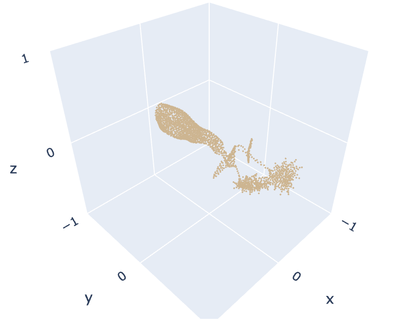
In Figure 7 we provide additional examples of randomly sampled transformations from each of our proposed data augmentation methods, which are the uniform orthogonal transformation, random RIP transformation, and smooth perturbation transformation.
Appendix G Failure cases



In Figure 6 we show examples from ModelNet40 that were misclassified by our method, and similar examples from the class it was misclassified as. The highest error rate ModelNet40 class is the flower pot class, which has an error rate much higher than any other class. Our method frequently mistakes the examples from the flower pot class for the plant class, which is much larger, and more rarely as other classes. As shown in Figure 6, examples from one class can be very similar visually to an example from another class, and we believe that this similarity is challenging for contrastive learning algorithms.


