New leptons with exotic decays: collider limits and dark matter complementarity
Abstract
We describe current and future hadron collider limits on new vector-like leptons with exotic decays. We consider the possibility that, besides standard decays, the new leptons can also decay into a Standard Model charged lepton and a stable particle like a dark photon. To increase their applicability, our results are given in terms of arbitrary branching ratios in the different decay channels. In the case that the dark photon is stable at cosmological scales we discuss the interplay between the dark photon and the vector-like lepton in generating the observed dark matter relic abundance and the complementarity of collider searches and dark matter phenomenology.
1 Introduction
New fermions are a common occurrence in models of physics beyond the Standard Model (SM). If they are vector-like delAguila:1982fs, namely both chiralities have the same quantum numbers, their mass term is gauge invariant and therefore it is not tied to the electroweak scale. As a result, they do not contribute to anomalies and all their physical effects decouple as inverse powers of their mass. Their phenomenological implications have been extensively studied, in particular in the case of vector-like quarks (triplets under color ), as they are strongly pair-produced at hadron colliders. Furthermore, the fact that electroweak top couplings have been measured with less accuracy than for lighter fermions leaves more room for relatively large indirect effects delAguila:2000rc; delAguila:2008pw and single production (see however Aguilar-Saavedra:2013qpa for strong constraints in minimal models and Anastasiou:2009rv for ways to evade them in more realistic ones).
Vector-like leptons (VLL), neutral under , have received much less attention. Indirect constraints deBlas:2013gla put very stringent limits on their mixing with the SM fermions, thus significantly reducing the possibility of a sizeable single production at colliders. Pair-production via Drell-Yan is quite model independent (see however Araque:2015cna; Araque:2015cbe; Chala:2020odv) but the smaller production cross-section than for vector-like quarks makes the reach quite modest (see Altmannshofer:2013zba; Falkowski:2013jya; Dermisek:2014qca; Kumar:2015tna; Bhattiprolu:2019vdu for theoretical studies and Aaboud:2018jiw; Aad:2015dha; Sirunyan:2019ofn for experimental searches). Furthermore, in all these cases, decays into only SM particles are assumed. However, there are classes of models with new VLL that incorporate a discrete symmetry under which SM particles are even and new particles are odd, thus preventing the decay of the VLL into only SM particles. They typically decay into the lightest odd-symmetric particle, which is often a dark matter (DM) candidate. A prime example is T-parity in Little Higgs models Cheng:2004yc; Low:2004xc. The lightest (and therefore easiest to produce) VLL usually decays into a SM lepton and a stable particle that results in missing energy at colliders. Such a decay has not been considered by experimental collaborations in the context of VLL searches. The production and decay pattern is very similar to the one of slepton pair production but due to the different spin of the particles involved, the interpretation of the experimental results in terms of VLL searches requires a recast of the analysis by theorists (see for instance Dercks:2018hgz).
Even more interestingly, the possibility of simultaneously having both types of decays, into a SM lepton plus a , or Higgs boson and into a SM lepton and missing energy, has never been considered in the past, despite the fact that this possibility is easy to realize and is even well motivated in the context of feebly interacting DM Delaunay:2020vdb. In this article we consider the possibility that the new VLL can simultaneously decay into the usual SM final states as well as into a SM lepton and missing energy. We will leave the decay pattern completely general so that our results apply to a large number of phenomenological models involving VLL. (See Chala:2017xgc for a similar study for the case of vector-like quarks.)
Inspired by the case of Little Higgs models with T-parity and by feebly interacting dark photon models we will consider the missing energy particle to be a dark photon, a massive vector that is stable at detector scales. However, this dark photon could be stable at much longer scales, of the order of the lifetime of the Universe and therefore be a good DM candidate. We will also explore this possibility and we will show that the VLL can play a crucial role in this regard. Indeed, it can open a large region of the allowed parameter space by either contributing to the relic abundance via co-annihilation with the dark photon or via the freeze-in mechanism. We will analyze these two possibilities and we will show that they can give complementary information in the former case and benefit from the collider searches in the latter one.
The rest of this article is organized as follows. We describe in Section 2 the most relevant current experimental searches for a new VLL with general decays. We then optimize these searches and obtain the expected LHC bounds on new VLL with arbitrary branching ratios with the current recorded luminosity. This is one of the main results of this article and it allows us to immediately get the constraints on new VLL with arbitrary decay patterns. We then explore the reach of the high-luminosity (HL-LHC) and high-energy (HE-LHC) configurations of the LHC together with an estimation of the final hh-FCC reach. Section 3 is devoted to the case in which the missing energy particle is stable and can act as a good DM candidate, first assuming the standard freeze-out mechanism and then the freeze-in one. We will see that in both cases the interplay with the VLL is crucial for a successful model. We then present our conclusions in Section 4. We present in Appendix A an explicit realization of the scenario we consider in the main text.
2 New vector-like leptons with general decays
The goal of this article is to study the current and future reach of hadron colliders on new VLL that can decay not only into SM particles but also into a SM charged lepton and a neutral particle that is stable at detector scales and therefore appears as missing energy. We will present our results in a model-independent way whenever possible, as a function of arbitrary branching ratios in the different channels. To show actual limits we will however focus on a new VLL singlet with electric charge -1, , and mass , and a massive vector boson , as the stable (at detector scales) particle, with mass so that can decay into and a SM lepton.
An explicit realization of our model is given in Appendix A but the details are not needed for the moment. The only relevant information is that the dominant decays are given by the following branching ratios , , and , where stands for either electron or muon11 1 Decays into tau leptons have been considered, assuming SM decays only, in delAguila:2010es; Kumar:2015tna; Bhattiprolu:2019vdu. and we assume the sum of these four branching ratios to be equal to one but otherwise arbitrary.22 2 The decays into SM particles are usually fixed by the quantum numbers of the VLL but in realistic models with a rich spectrum, the mixing between heavy states can lead to arbitrary decay patterns Chala:2013ega. We focus on Drell-Yan pair production, with subsequent decays governed by the corresponding branching ratios.33 3 Studies in which the production and/or decay of new vector-like fermions are dominated by non-renormalizable interactions can be found in Criado:2019mvu; Chala:2020odv. Out of the four possible decay channels, the two that are easiest to detect experimentally are and . The charged current one into is difficult to disentangle from the overwhelming background and the one into is either also difficult to disentangle from the relevant background or suffers from small branching fractions into easier to detect channels. Thus, in the following we will focus on the cleaner channels and give our results in terms of and . We will show that the results are mostly insensitive to the value of the two extra branching ratios.
There are currently two experimental analyses that are most sensitive to these discovery channels, searches for VLL into and slepton searches. Neither of them can be directly used in our more general scenario, except for the former in the limit. The slepton searches have to be completely recast because of the different spin of the intermediate particle and also because of the contamination of other channels in the limit.
We will begin this section by recasting the two relevant experimental analyses. We will first compare our results with the ones published by the experimental collaborations and then extend the analyses by considering arbitrary decays into the different channels. We will also update the analyses to take full advantage of higher luminosity and/or center of mass energy.
2.1 Recasting existing analyses
Since our goal is to interpolate between the limiting cases in which the branching ratio of the VLL to the missing energy channel goes from 0 to 1, we start by reproducing searches that probe these two limiting cases. The VLL model is implemented in Feynrules Alloul:2013bka and leading order event generation is done with MadGraph5_aMC@NLO Alwall:2014hca. For the background simulation generator level cuts are applied which are specified in the text. All of these were tested to verify that their influence was minimal to the final yield of events after the analysis. Showering and hadronization are performed by Pythia8 Sjostrand:2014zea with the CMS CUETP8M1 Khachatryan:2015pea underlying event tuning and the NNPDF23LO Ball:2012cx parton distribution functions. The detector response is modeled with Delphes 3 deFavereau:2013fsa. We use the default CMS card for the LHC analysis and the HL-LHC detector card for the analysis. C.L. limits are obtained using the Read:2002hq method by fitting the relevant discriminant variables using OpTHyLic Busato:2015ola which outputs the upper limit on the signal strength, , where is the upper limit on the cross-section and is the theoretical prediction obtained through the MadGraph simulation.
2.1.1 Decays into SM particles
For the case in which the VLL decays exclusively to SM final states (, and ) we reproduce the analysis presented in Ref. Aad:2015dha, an ATLAS search performed at and an integrated luminosity of , looking for multi-lepton signals coming from the decay of a singlet VLL. The main production and decay channels are depicted in Figure 1. This analysis selects 2 opposite sign same flavour (OSSF) leptons to reconstruct a boson and a third lepton with a , with and the pseudo rapidity and azimuthal angle, respectively, from the reconstructed boson, which is defined as the off- lepton. The definition of the full cuts and the corresponding efficiencies are presented in Table 1.
| Selection Cuts | |||||
|---|---|---|---|---|---|
|
0.25 | 0.19 | 0.0024 | ||
| 0.25 | 0.19 | 0.0023 | |||
| 0.17 | 0.11 | 0.0008 |
The analysis searches for an excess in the distribution of the variable , where the mass of the reconstructed boson, denoted by , is subtracted from the invariant mass of the 3-lepton system, . Furthermore, 3 exclusive signal regions are defined, depending on the number of identified leptons and hadronically decaying : 4-lepton region, in which at least 4 leptons are identified; 3-lepton + region, in which precisely 3 leptons are identified together with 2 jets whose invariant mass must be in the range , with the boson mass; and 3-lepton only region, in which exactly 3 leptons are identified with no pairs of jets satisfying the previous condition on their invariant mass.
The analysis is performed separately for the case in which the off- lepton is an electron or a muon, corresponding to the VLL coupling only to first or second generation leptons, respectively. The main backgrounds for this analysis are , and , for which our simulation very accurately reproduces the shape. We normalize these backgrounds to the values reported in the experimental publication, which amounts to a factor between 1.4 and 3.5, depending on the signal region, including the corresponding K-factor. We show in Figure 2 the comparison of our 1- and 2-sigma exclusion plot (Brazilian plot) with the expected limit reported in the experimental search, together with the theoretical pair production of the VLL, for the case in which the off- lepton is an electron. The case in which it is a muon shows a similar level of agreement. In this analysis the VLL branching fractions are fixed to those of an electroweak singlet (as a function of its mass) and the resulting limit on the VLL mass is , which represents a difference of in comparison to the expected limit obtained in original analysis.
Selection cuts A B C A B C A B C OSSF lepton pair with 0.25 0.25 0.25 0.18 0.18 0.18 0.48 0.48 0.48 0.16 0.16 0.16 0.10 0.10 0.10 0.14 0.14 0.14 0.054 0.029 0.0098 0.029 0.015 0.0052 0.05 0.02 0.01 0.054 0.025 0.0073 0.029 0.012 0.0035 0.05 0.02 0.01 0.054 0.025 0.0067 0.029 0.012 0.0031 0.05 0.02 <0.01 off- lepton = 0.029 0.013 0.0034 0.013 0.0053 0.0014 0.03 0.01 <0.01 () 0.0079 0.0043 0.0014 0.0013 0.0009 0.0004 0.01 0.01 <0.01
In order to see what the reach with the current recorded luminosity can be we have repeated the same analysis at and . However, we can take advantage of the higher center of mass energy to impose more stringent cuts, in particular on the transverse momentum of the leading leptons. Since the of the observed leptons in signal events increases with the increase in the VLL mass, we have defined 3 clusters of masses in which the selection threshold for of observed leptons varies. We present in Table 2 the definition of these clusters and the efficiencies of all selection cuts. With these more stringent selections, we were able to apply generation level cuts on the background, generating only events in which at least one lepton has .
Furthermore, at these higher energies, we can also remove almost the entirety of the background by setting a cut on the transverse mass, , of the reconstructed boson. This cut is effective because in events from , in principle, the off- lepton is coming from the decay and the missing energy of the event, , originates from the neutrino. Therefore, for events from the background, we have
| (1) |
where is the transverse momentum of the off- lepton. As such, this quantity should, in principle, be at most the mass of the boson. In order to keep as many signal events as possible, this cut is only performed on the 3-lepton signal region, which contains most of the background. Figure 3 shows the limits obtained with this improved analysis. Assuming that the observed data corresponds to the expected background, a mass of the VLL up to () could be excluded by this analysis for the case in which the off- lepton is an electron (muon). Given the similarity between the limits obtained when the VLL couples to first or second generation of SM leptons, we will only explore the case in which it couples to electrons hereafter.
Despite being tailored for the case in which the VLL is a singlet of , this analysis can also be applied for a VLL doublet, , of hypercharge . In this case we need to take into account not only the pair production of the charged component of the VLL doublet, , but also the pair production of the neutral component, , and the associated production of both, . For large masses (we will consider both components degenerate in mass), the charged component will decay equally to and , while the neutral component decays solely to . Therefore, our background remains the same, and as such we can recast the previous analysis to the doublet case, obtaining the limits shown in Figure 4, where we considered the off- lepton to be an electron. As expected, we obtain much more stringent bounds than on the singlet case, with masses up to being excluded.
An analysis searching for VLL doublets of hypercharge was performed by the CMS collaboration in Ref. Sirunyan:2019ofn with an integrated luminosity . A bound was obtained in this analysis due to a statistical fluctuation in the observed data. The expected limit in that analysis, which is the fair comparison to the bound we can compute, corresponded to . Rescaling our search to the same integrated luminosity we find , remarkably close to the expected limit in the CMS search, despite the fact that the CMS analysis targets decays into tau leptons and therefore a direct comparison is not straight-forward.
2.1.2 Decays with missing energy
To explore the case in which the VLL decays predominantly into a SM lepton and missing energy ( in our case), we consider an ATLAS analysis Aaboud:2018jiw at and an integrated luminosity of searching for pair produced sleptons decaying into a SM lepton and a neutralino, as represented in Figure 5. The analysis selects events with 2 OSSF leptons (, ), imposing a veto on additional jets. It also rejects events with an invariant mass of the two leptons . Several inclusive and exclusive signal regions are defined in which different requirements are demanded for and the variable Barr:2003rg; Lester:1999tx, defined by
| (2) |
where represent the transverse momentum of each of the identified leptons and is the vector that minimizes the maximum of both transverse masses, defined as
| (3) |
The main backgrounds for this signal are diboson processes (, and ) and . In order to maximize our statistics we always include 2 leptons (with an partonic cut) in the final state in the background generation. These 2 leptons can be of either family for the diboson case and are restricted to the first two generations for the one. The selection cuts and corresponding efficiencies are presented in Table 3. We have validated the analysis including all signal regions proposed in the original analysis Aaboud:2018jiw. However, new results are calculated considering only the signal region of and as we find the difference in regards to all signal regions not significant. Given that the analysis in Ref. Aaboud:2018jiw applies to sleptons and neutralinos, which are scalars and fermions, respectively, as opposed to our case with a VLL and a dark photon (fermion and vector, respectively), in order to validate our analysis we have implemented a slepton-neutralino model. Fixing the neutralino mass we obtain the results shown in Figure 6, with a limit , very similar to the expected limit obtained by the ATLAS collaboration, .
| Selection Cuts | |||||
|---|---|---|---|---|---|
|
0.33 | 0.33 | 0.23 | 0.53 | |
| 0.31 | 0.28 | 0.11 | 0.53 | ||
| 0.31 | 0.28 | 0.11 | 0.53 | ||
| 0.28 | 0.26 | 0.095 | 0.51 | ||
| 0.24 | 0.24 | 0.093 | 0.13 | ||
| 0.15 | 0.14 | 0.081 | 0.061 | ||
| 0.0064 | 0.003 | 0.0002 | 0.0001 | ||
| 0.0016 | 0.001 | 0.0002 | 0.0001 |
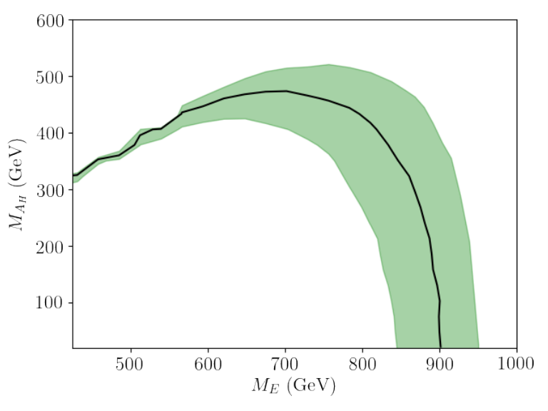
Once we have validated the analysis we can apply it to the VLL model. Contrary to the case of purely SM decays, in this case we have a new degree of freedom in our analysis, the mass of the other new particle, . Some models predict this mass to be close to the electroweak scale, such as the Littlest Higgs model with T-parity, but in other cases, we can have sub-GeV masses as is the case in feebly interacting massive particles (FIMP) in which this new particle plays the role of DM as we will see below. As such for each mass point of the VLL, we vary from 1 GeV up to the mass of the VLL in question. We present the limits obtained for and an integrated luminosity in Figure 7. As expected, the analysis is more constraining for lighter . As the mass difference between and the VLL decreases, the leptons from signal events become softer and more difficult to identify and pass the selection cuts. For the production cross-section is too low and the analysis cannot constrain the signal regardless of .
2.2 Constraints on vector-like leptons with general decays
Once we have ensured the accuracy of our simulations to recast the experimental searches in the limiting cases in which the VLL decays only through SM or missing energy channels, we are in a position to interpolate between them and therefore consider the case of arbitrary branching fractions in the different channels. To do this, we have scanned different possible branching ratios for each of the decay channels. In order to not need to generate every signal corresponding to different BRs, we apply a weight to each signal event according to its decay. To do this, we generate a signal of Drell-Yan pair-produced VLLs with , where the subscript describes the generated sample. To probe a specific point with different BRs, each event is weighted by , where subscript represents the probed branching ratio and superscript corresponds the specific decay – the decay of each event is determined at generator level.
Which analysis is more constraining depends on the particular value of the branching ratios but since they specifically target the final states with either and , the results are presented in the plane with the others branching ratios being fixed to
| (4) |
which correspond to the relation between the different branching ratios in the large limit for . We have checked that the corresponding bounds are quite insensitive to this latter choice. The residual dependence is due to cross-contamination between different channels into our signal regions. However, this effect is small as shown in Figure 8, where we represent the change in the signal strength as a function of the branching ratio into for two different values of the remaining parameters. The signal strength that represent our discriminating variable changes by at most, which results in a very mild dependence of the final limit on .
Our final result, that combines the two analyses discussed in the previous section for arbitrary values of and are shown in Figure 9 for two different values of (left panel) and (right panel). As expected, the effect of the mass is more relevant in the region in which the missing energy signal dominates and for lighter values of the VLL mass, since the smaller mass difference results in a softer lepton. Still, except for very low branching ratios into the decay channels targeted by our analysis, the differences are minimal. Thus, from now on we will only report our results for . We show the results as contours for fixed value of with the region above and to the right of each contour line being excluded for that mass at the CL. The limit for the VLL singlet case with SM decays can be easily obtained by considering the vertical axis, which corresponds to , at the relevant (mass dependent) . The most stringent bounds are along both axes, when the branching ratios into the channels we are most sensitive to are maximized. The numerical value of the limits in these three interesting cases are
| (5) |
2.3 Future projections
The constraints presented in Figure 9 represent the current constraints on a new charged VLL with general decays. In this section we explore the potential of the LHC to probe new VLLs in its high-luminosity (HL-LHC) and high-energy (HE-LHC) configurations. We will also explore the potential reach of the 100 TeV hh-FCC.
Starting with the HL-LHC (for which we take and an integrated luminosity of ) we use the same improved analysis described in the previous section and in Table 2, making sure that we generate enough statistics for the required integrated luminosity. The result is shown, for , in Figure 10. The correspond final reach of the HL-LHC in the limiting cases of a VLL singlet, and is, respectively,
| (6) |
When considering a higher energy collider, like the HE-LHC, for which we consider and , we can again afford to impose more stringent cuts on the different variables involved in the analysis, in particular in the lepton . In the SM decays analysis, we impose a partonic cut on all backgrounds of of the leading lepton whereas for the analysis focusing on the missing energy decay, backgrounds were generated with a partonic cut of for the leading lepton. We were able to use this cut since we updated the selection thresholds from Table 3 to in the missing decay analysis. The resulting reach, again for , is reported for arbitrary branching ratios in Figure 11. The estimated reach, in the limiting cases is
| (7) |
A detailed study of the reach of future circular colliders on VLLs with general decays is beyond the scope of the present work, however, we can use a crude estimate of the corresponding reach at the hh-FCC by considering the instantaneous luminosity as used in the Collider Reach tool colliderreach. First we test the validity of this approach by extrapolating the current luminosity results reported in Eq. (5) to the HL-LHC and to the HE-LHC. We find that the extrapolation agrees with our detailed simulation within in the case of the HL-LHC for the SM decays analysis (missing decays analysis) and within for the HE-LHC for the SM decays analysis (missing decays analysis). The latter case shows the differences that arise not only from the increased production cross sections of signal and backgrounds but also from the more stringent cuts that we can imposed with higher energy. The difference in the missing decays analysis drops to 14 % when we extrapolate from the HL-LHC results. We can expect a similar effect when extrapolating our results to the FCC. Assuming and we obtain the results shown in Figure 12 and the following limits in the VLL, pure and pure decay cases
| (8) |
The results reported in Figures 9-12 are completely general except for the fact that we are using the production cross-section of a VLL singlet with hypercharge -1 to obtain the mass limits. For the sake of generality, we provide in Figure 13 the cross-sections we have used for the LHC, HE-LHC and hh-FCC so that our limits can be applied to more general VLLs by rescaling the corresponding pair production cross-section.
3 Dark photon as a dark matter candidate
So far we have just assumed that the lifetime of is large enough to appear as missing energy at detector scales. However, if has a lifetime larger than the age of the universe, it becomes a suitable candidate for DM. As such, we can use the observed relic density and direct detection experiments to further constrain these models. In this section we will focus on two possible production mechanisms for DM. We will first consider the case in which has a mass around the electroweak scale and its abundance is fixed through the freeze-out mechanism. Then we will consider the possibility that is light and has a very weak coupling to the SM so that its production follows the freeze-in mechanism.
3.1 Standard freeze-out
For the case of a heavy DM candidate – with a mass around the eletroweak scale – we will consider that it is stabilized through a symmetry. An example of this arises in the Littlest Higgs model with T-parity (LHT) Cheng:2004yc; Low:2004xc, in which is T-odd, as is the vector-like lepton, while the SM particles are T-even. Therefore, the VLL decays exclusively through the missing energy channel. Since is a singlet of the SM, we can write the following operators
| (9) |
where , the dots represent other couplings that are irrelevant for the viability of as a DM candidate and we have included explicit factors of the gauge coupling to make the connection with the LHT model more direct. In the LHT model and delAguila:2008zu.
The latest Planck results measured the relic density abundance to be Aghanim:2018eyx and therefore the model must predict a relic density equal to ( accounts for all of DM) or smaller than ( is only part of DM content) that number. The most relevant processes for the annihilation of are to b-quarks, or bosons or top quarks (depending on the mass of the DM candidate) through the s-channel exchange of a Higgs Birkedal:2006fz. Furthermore the annihilation into leptons through the exchange of the VLL is also important – the corresponding diagrams are shown in Figure 14. Therefore, as mentioned above, the relic density calculation will be controlled by the couplings of to the Higgs and the coupling to the VLL and SM lepton and thus we will scan different values for these couplings. Given that the VLL mediates one of these channels, when the s-channel annihilation is subdominant, the mass difference between and the VLL will also play an important role.
The calculation of the relic density is done using MadDM Ambrogi:2018jqj by inputting a UFO model Degrande:2011ua which we generate through Feynrules Alloul:2013bka. The results are presented in Figure 15 for a VLL mass in the plane for different values of . The curves represent the values for which the relic abundance agrees with the observed value. The region below the curve is excluded and the one above requires further sources of DM. We also show, shaded in grey, the excluded region from direct detection using the latest XENON1T data Aprile:2018dbl. For small values of (), the s-channel annihilation through the Higgs dominates; however, as we increase , the channel mediated by the VLL becomes more important and we get a significant rise in the annihilation cross-section, with a allowing almost all of the depicted parameter space. As expected, we can also see (particularly for high enough values of ) that, as the mass difference between the VLL and the DM candidate decreases, the impact of the VLL-mediated channel increases. The coupling to the Higgs boson is also important for the spin-independent scattering cross-section with nucleons, as the dominant diagrams are the Higgs exchange with quarks or with gluons through a loop of heavy quarks as represented in Figure 16. We have computed the corresponding scattering cross-section with MadDM and shown the excluded region in Figure 15.
Varying also affects direct detection constraints. In principle could be responsible for a 1-loop DM nucleon scattering amplitude, mediated by a photon. However, as noted in Ref. Agrawal:2014ufa, for the case of a real DM vector candidate, the coupling between 2 DM particles and a photon will be described by a dimension-6 operator, since the dimension-4 does not exist due to the antisymmetry of the field strength tensor. Moreover, the resulting amplitude will be further suppressed when one takes the non-relativistic limit. As such, we will neglect contributions from this process to direct detection bounds in this work.
Another experimental observable which may be affected by changing is the anomalous magnetic moment of both the electron and the muon, depending on which of these SM leptons the VLL couples to. The latest experimental results are Aoyama:2012wj; Muong-2:2021ojo
| (10) | ||||
| (11) |
where the uncertainties include theoretical and experimental contributions.
The new contribution from and reads Agrawal:2014ufa,
| (12) |
where and and is the mass of the SM lepton for which the contribution is being calculated. This result is always negative and as such, it contributes in the direction of explaining the anomaly of the electron, whereas it goes in the wrong direction for the muon anomaly. Figure 17 shows the parameter space that is constrained by these measurements. For the case in which the VLL couples to electrons, we show the region which explains the observed anomalous magnetic moment. For the muon case, as this model increases the tension with the experimental result we constrain this contribution to be smaller than the combination of the experimental and theoretical uncertainties. The region above the curves is excluded for the muon case.
The results shown in Figure 15 reflect the well known tension between the production of the correct relic abundance and direct detection experiments for a standard weekly interacting massive particle. Such tension can be relaxed if the masses of the new particles are nearly degenerate (with the VLL being slightly heavier). This regime of co-annihilation Baker:2015qna increases the annihilation cross-section since processes such as and can now contribute significantly. The importance of these contributions will be a function not only of this degeneracy in mass, but also of the coupling . An estimation of the needed mass splitting to have a significant contribution to the annihilation process can be obtained by considering that, at the freeze-out temperature, , both particles are still in equilibrium. For co-annihiliation to be important, one would have . Knowing that , for cold DM, the splitting must be at most where .
In Figure 18 we show the relic density abundance for cases in which co-annihilation can be important. We consider two values of (solid) and (dashed) and plot the contours of for different values of . The region to the right of the different curves is excluded (as it gives too large relic abundance). Again we show in shaded grey the region excluded by direct detection experiments. We see that only for a significant difference with respect to the standard annihilation scenario is observed.
In order to better understand the dependence on in this co-annihilation regime we show, in Figure 19, the contours in the plane, again for different values of for . The region excluded by direct detection experiments is, as usual, shaded in grey. While for fixed we observed that increasing collapses the relic density line into the non co-annihilation regime, this does not happen in this plot. In this case, even though co-annihilation effects can be negligible for , the annihilation process mediated by the heavy lepton is important for low mass differences between the VLL and and large and as such the annihilation cross-section is influenced by changes in even outside the co-annihilation regime.
Note that this co-annihilation case is complementary to what was studied in the previous section at colliders. In this case, given the small mass difference, the final state leptons at colliders will be very soft and therefore are very difficult to identify. There is an ongoing effort to search for this cases of compressed mass states at colliders ATLAS:2019lng namely in the context of sleptons. Our results show that the interpretation of such a search in the context of VLLs is very well motivated.
3.2 Freeze-in in feebly interacting dark matter
In the case that DM is very light and couples very weakly to other particles, its relic density can be set by the freeze-in mechanism Hall:2009bx. In this case, the DM candidate is not in equilibrium with the thermal bath but is actually produced through the decay of other heavy particles, in our case, the decay of the VLL. This possibility has been recently explored in Delaunay:2020vdb with emphasis on the DM phenomenology, thus setting the VLL mass to a conservative in order to avoid any collider constraint. In this subsection we aim to show the complementarity between DM experiments and the collider results we presented before for a FIMP.
This scenario is realized by the explicit model that we present in Appendix A, to which we refer the reader for the details. The relic density can be calculated as Delaunay:2020vdb:
| (13) |
For each value of and the condition that corresponds to all of DM, i.e. Eq. (13) , fixes the product . Choosing then a value for fixes all branching ratios of the VLL. As such, by choosing a particular we can get the collider bound from our previous analysis.
We present these results in Figures 20 and 21 for the LHC analysis at and and respectively. The region below the curves can be excluded by collider searches. In the region above the curve, for that fixed value of , all the values of and are experimentally allowed and can provide the correct DM relic abundance. For each curve, we display it as a solid or dashed curve depending on whether the most constraining analysis is the one which is most sensitive to the decays into SM particles or into missing energy, respectively. This is relevant since, in order to use the collider bounds we obtained, must be a prompt decay for the missing energy search whereas is the most important channel to be prompt in the SM decays analysis.
In Eq. (38) we show the minimum value must take so that is prompt. For the value of (fixed for each mass point) is going to determine whether it is a prompt decay mode. In Figures 20 and 21 we show, in shaded gray, the regions in which the decay length is (light gray) or (dark gray). This is relevant for the dashed part of the curves and shows that, for smaller values of , the limits on might be significantly weaker. A more detailed analysis, which is beyond the scope of the present work, targeting displaced vertices has the potential to significantly probe the allowed region of parameter space in this class of models.
4 Conclusions
New vector-like leptons are quite common in extensions of the Standard Model. In minimal extensions, with no further new particles or anomalous couplings, their decays are governed by their mixing with the Standard Model leptons, which is strongly constrained by electroweak precision data. These constraints eliminate the possibility of substantial single production, leaving Drell-Yan pair production as their dominant production mechanism. Realistic new physics models are, however, usually far from minimal and the new particles present in the spectrum can have a significant impact on the phenomenology of these new leptons. New stable particles allow the possibility of a decay of the vector-like lepton into a Standard Model charged lepton and missing energy. Such a signature has been only experimentally searched for in the context of supersymmetric models with slepton pair production decaying into leptons and neutralinos. From the information given in the experimental analyses it is difficult to directly translate the corresponding bounds to the vector-like lepton case, despite the fact that this signature is well motivated by natural models like the Little Higgs models with T parity. Furthermore, the case in which the new lepton can simultaneously decay into Standard Model particles and into a Standard Model charged lepton and missing energy has been never considered before. This possibility is however also well motivated as it naturally appears in models of feebly interacting dark matter models in which the dark matter relic abundance is generated via the freeze-in mechanism.
In order to fill this gap we have considered the possibility of a new charge -1 vector-like lepton that can decay, with arbitrary branching ratios into a Standard Model lepton together with a , , or missing energy, represented by a dark photon , which is assumed to be stable at detector scales. We have then considered the most relevant LHC analyses probing such a model and, after carefully validating our implementation of the analyses, we have computed the current and future constraints that hadron colliders can place on new vector-like leptons with these exotic decays. Our results, represented as mass limits as functions of and are provided in Figures 9-12 for current data at the LHC, the HL-LHC, the HE-LHC and the 100 TeV hh-FCC, respectively. This is one of the main results of our work, as it provides the experimental limits from current and future hadron colliders on a large number of models of vector-like leptons with exotic decays.
We have also considered the interesting possibility that the dark photon, , is not only stable at detector scales but also at cosmological scales. It can then be a good dark matter candidate and we have explored the interplay between the dark photon and the vector-like lepton to provide a successful explanation for the observed dark matter relic abundance. After showing that the standard freeze-out mechanism presents tension between the generation of the dark matter relic abundance and limits from direct detection experiments, leaving only a relatively small region of viable parameter space, we consider the case of near degeneracy between the vector-like lepton and the dark photon. This leads to a successful generation of dark matter via co-annihilation, compatible with all current experimental limits. The relevant region of parameter space is complementary to collider searches, as the compressed spectrum significantly deteriorates the collider reach. The possibility of specific searches that target these compressed spectra models becomes a very interesting probe of the model in this regime.
Finally, we have considered the case in which the dark photon is very light and feebly interacting, realizing the freeze-in mechanism. We have shown that in this case collider searches are very complementary to dark matter probes and we have found that models compatible with current dark matter phenomenology can be easily tested in current or future hadron colliders.
Acknowledgments
We are grateful to N. Castro, M. Chala, M. Ramos and T. Vale for useful comments. This work has been supported in part by the Ministry of Science, Innovation and Universities (PID2019-106087GB-C22) and and by the Junta de Andalucía grants FQM 101, SOMM17/6104/UGR, A-FQM-211-UGR18 and P18-FR-4314 (FEDER). GG acknowledges support by LIP (FCT, COMPETE2020-Portugal2020, FEDER, POCI-01- 0145-FEDER-007334) as well as by FCT under project CERN/FIS-PAR/0024/2019 and under the grant SFRH/BD/144244/2019.
Appendix A Explicit realization
We describe in this appendix an explicit realization of the framework used in this work. Rather than aiming at full generality we focus on a minimal model capable of generating the range of branching ratios we can be sensitive to at the LHC and future colliders. The explicit realization we describe here is well motivated as a good candidate for feebly interacting DM Delaunay:2020vdb. 44 4 Indeed our model corresponds to the one in Delaunay:2020vdb with the following replacements: . The model has an gauge symmetry. The matter fields consist of the SM particles, which are all neutral under , a new vector-like lepton with the following quantum numbers, with notation ,
| (14) |
and a complex scalar
| (15) |
At the renormalizable level we can write the following Lagrangian
| (16) |
where is a suitable potential to spontaneously break and to make the physical Higgs scalar of such breaking much heavier than all the other fields in the spectrum so that we can effectively neglect it. For simplicity we have assumed that kinetic mixing between the two abelian groups is negligible 55 5 The order of magnitude expectation for kinetic mixing Holdom:1985ag is small enough to be negligible for most of the parameter space and also well within the experimental limits Chun:2010ve. For values of on the smaller side a small extra suppression might be needed Gherghetta:2019coi. and that the VLL only couples to one of the SM RH charged leptons, taken to be the electron here, denoted by but it could equally well be the muon or tau, in the basis of diagonal charged lepton Yukawa couplings. Hereafter we suppress all terms in the Lagrangian that are not relevant for our discussion. The covariant derivative for the new fields reads
| (17) |
where we have used .
Once is spontaneously broken, the corresponding gauge boson, , acquires a mass
| (18) |
where we have denoted the vacuum expectation value (vev) of , and and mix
| (19) |
This mixing can be rotated away (thus defining the SM RH charged lepton) via the following unitary rotation
| (20) |
where
| (21) |
Denoting we have the SM extended with a VLL singlet with hypercharge and the following mass Lagrangian for the charged leptons
| (22) |
where and are generated after EWSB and satisfy
| (23) |
and a new neutral heavy gauge boson with couplings
| (24) |
The effect of mixing with extra vector-like fermions is well known delAguila:1982fs. The physical basis is obtained by diagonalizing the mass matrix in (22) via a bi-unitary rotation
| (25) |
where denotes the chirality and, in the limit that we will be interested in we have
| (26) |
where the dots denote higher orders in . The corresponding masses are
| (27) |
In this physical basis, the coupling of fermions to the electroweak gauge bosons, , , the Higgs boson, , and the heavy photon, , can be written as follows
| (28) |
where is a fermion of electric charge , is the gauge coupling, is the cosine of the weak angle and are flavor indices. The relevant couplings are, to leading order in the small expansion parameter,
| (29) |
where is the Higgs vev, denotes the neutrino flavor and we have suppressed all input that is not directly relevant for our purposes.
In order to realize our scenario we consider the limit , so that can decay into , , and and can decay into provided . The corresponding decay widths are
| (30) | ||||
| (31) | ||||
| (32) | ||||
| (33) |
where we have shown the leading terms in the , with , except for , for which the subleading term is relevant for low values of . Using the properties
| (34) |
we recover the standard decay pattern into , and for large values of . Finally, assuming we have
| (35) |
In order to realize our framework we need to be stable at detector scales, to decay promptly, and the branching ratios of decaying into and the SM bosons to be of similar order. Assuming a decay length larger than for and smaller than for , these conditions translate into
| (36) | ||||
| (37) |
Using the expressions above we can find, for each value of and , the values of and that satisfy these conditions. Indeed, requiring prompt decays gives lower bound on
| (38) |
Requiring that decays invisibly and the decay is prompt provides in turn an upper limit on
| (39) |
This upper limit is of the same order of magnitude as the one from electroweak precision data deBlas:2013gla. Note that for the values of we are sensitive to, unless is very close to , the two limits are always compatible. Provided is fixed in the allowed range, we can fix a minimum value of by requiring to be prompt
| (40) |
and a maximum one by requiring to be stable at detector scales
| (41) |
Once and are fixed within the allowed values we have fixed the relative decay of into and
| (42) |
Using the minimum and maximum values of we get
| (43) |
As an example, fixing and we have
| (44) |
Fixing for instance we now have
| (45) |
and
| (46) |
Considering the muon instead of the electron increases by a factor and reduces the lower limit of by a factor .
References
- (1) F. del Aguila and M. J. Bowick, The Possibility of New Fermions With I = 0 Mass, Nucl. Phys. B 224 (1983) 107.
- (2) F. del Aguila, M. Perez-Victoria and J. Santiago, Observable contributions of new exotic quarks to quark mixing, JHEP 09 (2000) 011 [hep-ph/0007316].
- (3) F. del Aguila, J. de Blas and M. Perez-Victoria, Effects of new leptons in Electroweak Precision Data, Phys. Rev. D 78 (2008) 013010 [0803.4008].
- (4) J. A. Aguilar-Saavedra, R. Benbrik, S. Heinemeyer and M. Pérez-Victoria, Handbook of vectorlike quarks: Mixing and single production, Phys. Rev. D 88 (2013) 094010 [1306.0572].
- (5) C. Anastasiou, E. Furlan and J. Santiago, Realistic Composite Higgs Models, Phys. Rev. D 79 (2009) 075003 [0901.2117].
- (6) J. de Blas, Electroweak limits on physics beyond the Standard Model, EPJ Web Conf. 60 (2013) 19008 [1307.6173].
- (7) J. P. Araque, N. F. Castro and J. Santiago, Interpretation of Vector-like Quark Searches: Heavy Gluons in Composite Higgs Models, JHEP 11 (2015) 120 [1507.05628].
- (8) J. P. Araque, N. F. Castro and J. Santiago, Interpretation of vector-like quark searches: the case of a heavy gluon in composite Higgs models and vector-like quarks, PoS TOP2015 (2015) 069 [1512.04744].
- (9) M. Chala, P. Kozów, M. Ramos and A. Titov, Effective field theory for vector-like leptons and its collider signals, Phys. Lett. B 809 (2020) 135752 [2005.09655].
- (10) W. Altmannshofer, M. Bauer and M. Carena, Exotic Leptons: Higgs, Flavor and Collider Phenomenology, JHEP 01 (2014) 060 [1308.1987].
- (11) A. Falkowski, D. M. Straub and A. Vicente, Vector-like leptons: Higgs decays and collider phenomenology, JHEP 05 (2014) 092 [1312.5329].
- (12) R. Dermisek, J. P. Hall, E. Lunghi and S. Shin, Limits on Vectorlike Leptons from Searches for Anomalous Production of Multi-Lepton Events, JHEP 12 (2014) 013 [1408.3123].
- (13) N. Kumar and S. P. Martin, Vectorlike Leptons at the Large Hadron Collider, Phys. Rev. D 92 (2015) 115018 [1510.03456].
- (14) P. N. Bhattiprolu and S. P. Martin, Prospects for vectorlike leptons at future proton-proton colliders, Phys. Rev. D 100 (2019) 015033 [1905.00498].
- (15) ATLAS collaboration, Search for electroweak production of supersymmetric particles in final states with two or three leptons at TeV with the ATLAS detector, Eur. Phys. J. C 78 (2018) 995 [1803.02762].
- (16) ATLAS collaboration, Search for heavy lepton resonances decaying to a boson and a lepton in collisions at TeV with the ATLAS detector, JHEP 09 (2015) 108 [1506.01291].
- (17) CMS collaboration, Search for vector-like leptons in multilepton final states in proton-proton collisions at = 13 TeV, Phys. Rev. D 100 (2019) 052003 [1905.10853].
- (18) H.-C. Cheng and I. Low, Little hierarchy, little Higgses, and a little symmetry, JHEP 08 (2004) 061 [hep-ph/0405243].
- (19) I. Low, T parity and the littlest Higgs, JHEP 10 (2004) 067 [hep-ph/0409025].
- (20) D. Dercks, G. Moortgat-Pick, J. Reuter and S. Y. Shim, The fate of the Littlest Higgs Model with T-parity under 13 TeV LHC Data, JHEP 05 (2018) 049 [1801.06499].
- (21) C. Delaunay, T. Ma and Y. Soreq, Stealth decaying spin-1 dark matter, JHEP 02 (2021) 010 [2009.03060].
- (22) M. Chala, Direct bounds on heavy toplike quarks with standard and exotic decays, Phys. Rev. D 96 (2017) 015028 [1705.03013].
- (23) F. del Aguila, A. Carmona and J. Santiago, Tau Custodian searches at the LHC, Phys. Lett. B 695 (2011) 449 [1007.4206].
- (24) M. Chala and J. Santiago, Hbb production in composite Higgs models, Phys. Rev. D 88 (2013) 035010 [1305.1940].
- (25) J. C. Criado and M. Perez-Victoria, Vector-like quarks with non-renormalizable interactions, JHEP 01 (2020) 057 [1908.08964].
- (26) A. Alloul, N. D. Christensen, C. Degrande, C. Duhr and B. Fuks, FeynRules 2.0 - A complete toolbox for tree-level phenomenology, Comput. Phys. Commun. 185 (2014) 2250 [1310.1921].
- (27) J. Alwall, R. Frederix, S. Frixione, V. Hirschi, F. Maltoni, O. Mattelaer et al., The automated computation of tree-level and next-to-leading order differential cross sections, and their matching to parton shower simulations, JHEP 07 (2014) 079 [1405.0301].
- (28) T. Sjöstrand, S. Ask, J. R. Christiansen, R. Corke, N. Desai, P. Ilten et al., An introduction to PYTHIA 8.2, Comput. Phys. Commun. 191 (2015) 159 [1410.3012].
- (29) CMS collaboration, Event generator tunes obtained from underlying event and multiparton scattering measurements, Eur. Phys. J. C 76 (2016) 155 [1512.00815].
- (30) R. D. Ball et al., Parton distributions with LHC data, Nucl. Phys. B 867 (2013) 244 [1207.1303].
- (31) DELPHES 3 collaboration, DELPHES 3, A modular framework for fast simulation of a generic collider experiment, JHEP 02 (2014) 057 [1307.6346].
- (32) A. L. Read, Presentation of search results: The CL(s) technique, J. Phys. G 28 (2002) 2693.
- (33) E. Busato, D. Calvet and T. Theveneaux-Pelzer, OpTHyLiC: an Optimised Tool for Hybrid Limits Computation, Comput. Phys. Commun. 226 (2018) 136 [1502.02610].
- (34) A. Barr, C. Lester and P. Stephens, m(T2): The Truth behind the glamour, J. Phys. G 29 (2003) 2343 [hep-ph/0304226].
- (35) C. Lester and D. Summers, Measuring masses of semiinvisibly decaying particles pair produced at hadron colliders, Phys. Lett. B 463 (1999) 99 [hep-ph/9906349].
- (36) G. Salam and A. Weiler, “Collider Reach.” http://collider-reach.web.cern.ch/.
- (37) F. del Aguila, J. I. Illana and M. D. Jenkins, Precise limits from lepton flavour violating processes on the Littlest Higgs model with T-parity, JHEP 01 (2009) 080 [0811.2891].
- (38) Planck collaboration, Planck 2018 results. VI. Cosmological parameters, 1807.06209.
- (39) A. Birkedal, A. Noble, M. Perelstein and A. Spray, Little Higgs dark matter, Phys. Rev. D 74 (2006) 035002 [hep-ph/0603077].
- (40) F. Ambrogi, C. Arina, M. Backovic, J. Heisig, F. Maltoni, L. Mantani et al., MadDM v.3.0: a Comprehensive Tool for Dark Matter Studies, Phys. Dark Univ. 24 (2019) 100249 [1804.00044].
- (41) C. Degrande, C. Duhr, B. Fuks, D. Grellscheid, O. Mattelaer and T. Reiter, UFO - The Universal FeynRules Output, Comput. Phys. Commun. 183 (2012) 1201 [1108.2040].
- (42) XENON collaboration, Dark Matter Search Results from a One Ton-Year Exposure of XENON1T, Phys. Rev. Lett. 121 (2018) 111302 [1805.12562].
- (43) P. Agrawal, Z. Chacko and C. B. Verhaaren, Leptophilic Dark Matter and the Anomalous Magnetic Moment of the Muon, JHEP 08 (2014) 147 [1402.7369].
- (44) T. Aoyama, M. Hayakawa, T. Kinoshita and M. Nio, Tenth-Order QED Contribution to the Electron g-2 and an Improved Value of the Fine Structure Constant, Phys. Rev. Lett. 109 (2012) 111807 [1205.5368].
- (45) Muon g-2 collaboration, Measurement of the Positive Muon Anomalous Magnetic Moment to 0.46 ppm, Phys. Rev. Lett. 126 (2021) 141801 [2104.03281].
- (46) M. J. Baker et al., The Coannihilation Codex, JHEP 12 (2015) 120 [1510.03434].
- (47) ATLAS collaboration, Searches for electroweak production of supersymmetric particles with compressed mass spectra in 13 TeV collisions with the ATLAS detector, Phys. Rev. D 101 (2020) 052005 [1911.12606].
- (48) L. J. Hall, K. Jedamzik, J. March-Russell and S. M. West, Freeze-In Production of FIMP Dark Matter, JHEP 03 (2010) 080 [0911.1120].
- (49) B. Holdom, Two U(1)’s and Epsilon Charge Shifts, Phys. Lett. B 166 (1986) 196.
- (50) E. J. Chun, J.-C. Park and S. Scopel, Dark matter and a new gauge boson through kinetic mixing, JHEP 02 (2011) 100 [1011.3300].
- (51) T. Gherghetta, J. Kersten, K. Olive and M. Pospelov, Evaluating the price of tiny kinetic mixing, Phys. Rev. D 100 (2019) 095001 [1909.00696].