IntraLoss: Further Margin via Gradient-Enhancing Term for Deep Face Recognition
Abstract
Existing classification-based face recognition methods [2, 21, 23, 9] have achieved remarkable progress, introducing large margin into hypersphere manifold to learn discriminative facial representations. However, the feature distribution is ignored. Poor feature distribution will wipe out the performance improvement brought about by margin scheme. Recent studies [28, 3] focus on the unbalanced inter-class distribution and form a equidistributed feature representations by penalizing the angle between identity and its nearest neighbor. But the problem is more than that, we also found the anisotropy of intra-class distribution. In this paper, we propose the ‘gradient-enhancing term’ that concentrates on the distribution characteristics within the class. This method, named , explicitly performs gradient enhancement in the anisotropic region so that the intra-class distribution continues to shrink, resulting in isotropic and more compact intra-class distribution and further margin between identities. The experimental results on LFW, YTF and CFP-FP show that our outperforms state-of-the-art methods by gradient enhancement, demonstrating the superiorty of our method. In addition, our method has intuitive geometric interpretation and can be easily combined with existing methods to solve the previously ignored problems.
1 Introduction
For the past few years, Deep Convolutional Neural Networks has greatly boost-ed state-of-the-art in Face Recognition, which makes deep CNN a primary way for the problem. Face Recognition, as one of the most common computer vision task, consists of two sub-tasks: face identification and face verification. Face identification, a one-to-many task, assigns a known identity to a given facial image from database. And face verification, a one-to-one task, determines whether a pair of facial images comes from the same identity. For testing protocols, according to the consistency of identity of training set and test set, it can be divided into two kinds: 1) Open-set protocol, where testing identities may not come from training set, and 2) Close-set protocl, where training set and testing set have the same identities. Face Recognition can be regarded as classification tasks or metric learning tasks. Under the premise of close-set protocol, face recognition is viewed as a classification task, and the face identity is directly output via softmax layer. While from the perspective of open-set, face recognition is more like a metric learning task, and the corresponding identity is obtained by performing feature comparison with the identity in the database. Under such a circumstance, feature extractor requires more discriminative capabilities, which means that features of the same class are as compact as possible(intra-class compactness), whereas features of different class are far enough apart(inter-class separability). It is obvious that open-set face recognition is closer to real-world use and applications, yet with more challenge.
A standard deep CNN-based face recognition pipline consists of four stages: face detection, face alignment, feature representation, and feature comparison. Early deep learning-based studies [20, 7, 18, 26], in the manner of multi-class classification problem, build deep convolutional neural networks to extract high-level facial features, used the softmax loss to supervise training procedure, and improve performance through elaborate network design and large scale dateset. Deepface [20] proposes a local convolution layer to learn different convolutional kernels for different positions on the feature map to adapt to different features in different regions of the face. DeepID [18] constructs a network with the last hidden layer connected to the third and fourth convolutional layers, and the dimension of the last hidden layer is fixed to 160, which is much smaller than the number of identities to form a compact and predictive feature representation. Deep CNNs learn from the data, and the scale of the data greatly affects the generalization performance. Recent years have presented several large-scale face datasets, such as CASIA-WebFace [26], LFW [7], MS-Celeb-1M [5], Youtube Face(YTF) [25], VGGFace [12]. More than that, data synthesis method [11] has also been published, further inreasing the amount of the data, improving the generalization performance and preventing overfitting.
Apart from the two factors above, loss function plays a ciritical role in determining the discriminative capability of learned facial representations. Through softmax loss, which is widely used to train deep CNNs, only separable feature representations can be learned, with limited discriminative capacity. For face recogniton, feature representations should be not only separable, but also discriminative. To motivate better discriminative feature performance, metric-based loss was introduced. Contrastive loss [1] and triplet loss [16] learn more efficient features directly from training pairs and triplets, leading to Euclidean margin(the largest intra-class distance is smaller than the shortest inter-class distance in Euclidean space). Nevertheless, the careful selection of pairs and triplets is very difficult and time-consuming, and it will inevitably significantly increase the computational complexity and cause slow convergence and instability.
In contrast, softmax loss has simple sampling and fast convergence, hence some works [17, 24] combine softmax loss and metric loss together to train CNNs. Furthermore, many classification-based research studies [10, 9, 14, 22, 23, 21, 2] has been proposed. [14, 22] normallize features and weights parameters and map them onto hypersphere manifold, and show that the normalization operation can boost the final performance. Based on this, SphereFace [9] imposes angular margin to hypersphere in a multiplicative way. More than that, AM-softmax [21, 23] and ArcFace [2] respectively improved softmax loss in the form of additive cosine margin and additive angular margin.
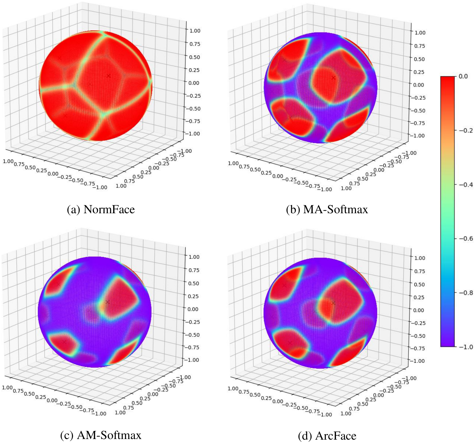
However, the above methods all focus on introducing margin into loss function to enhance the discriminative capacity, but neglect to consider the overall feature distribution on the hypersphere. Latest researches, such as RegularFace [28] and UniformFace [3] , point out that the inter-class distribution is highly nonuniform, which leads to less feature discrimination despite the large intra-class margin, and new objective functions are proposed to learn equidistributed feature representation. Beyond that, when we look at the intra-class distribution, we found another problem that the shape of each intra-class distribution is an anisotropic polygon, which is a system defect of all classification-based methods due to the anisotropy of the feature space partition when classifying. Geometrically speaking, when margin works, the origin classification decision boundaries are pushed closer to the center of each class. Accordingly, the intra-class distributiion becomes compacter, but the original distribution characteristics are maintained. The anisotropy makes, in different orientation, the same distance from class center brings about different gradients. We suggest that such a phenomenon will cause incomplete optimization of intra-calss distribution, and compromise the inter-class margin.
In this work, we focus on the other side of feature distribution: intra-class distribution, and propose a gradient-enhancing term, named IntraLoss, to impose a novel supervising signal upon hypersphere. This gradient-enhancing term explicitly restores gradient where gradient disappears farther away from the class center, resuming optimizing process. Consequently, the intra-class variations is further reduced, resulting in further margin on the hypersphere.
Our contributions are summarized as follows:
- •
First, we raise and discuss the problem of nonequivalent intra-class gradient distributions in different orientation on hypersphere manifold, and the accompanying problem of class center diviation.
- •
Second, we propose a novel gradient-enhancing term, called IntraLoss, which explicitly narrows intra-class variations to encourage further margin by restoring gradient. To be best of our knowledge, this is the first attempt to enhance feature discrimination by using such a loss objective on the hypersphere manifold.
- •
Third, our proposed gradient enhancing method is orthogonal with, and can be easily implemented into existing methods, and it is adaptive according to the distributiion of each class on the hypersphere with no extra hyperparameters introduced.
- •
2 Related work
To our best knowledge, based on the large margin loss functions in use, there are two major types methods: metric-based methods and classification-based methods.
2.1 Metric-Based Methods
The purpose of Metric-Based Methods are to obtain a similarity(semantic distance) function in Euclidean space through learning, reduce the distance between homogeneous samples, and increase the distance between different class of samples. For open-set face recognition, metric between samples directly determines the final result.
Metric Loss. Since the open-set face recognition is similar to metric learning, some works directly implement metric loss to Networks. Contrastive Loss [1] constructs a Siamese Networks to perform representation learning, and two facial images are fed into networks to obtain their respective feature representations. By penalizing the distance between image pairs, make the images of the same class as close as possible, and images of different classes are far enough. Moreover, Triplet Loss [16] accepts three facial images at once, two of which are from the same class (the anchor and positive) and the other from a different class (the negative). Triplet loss minimizes the distance between the same class, and maximizes the distance between different classes, bringing out that the largest intra-class distance is less than the smallest inter-class distance.
Joint Loss. Note that metric loss is difficult to converge, and needs careful and time-consuming sampling strategy. DeepID2 [17] forms a joint loss function based on DeepID’s network [18], which greatly improves performance. Concretely speaking, the original convolutional neural network used softmax loss as objective function, so-called identification signal. In DeepID2 [17], a verification signal, known as Contrastive loss, is introduced. The two signals are combined using a weighted manner. In regularization way, Center Loss [24] penalizes the distance between feature and the corresponding center to reduce the intra-class variations, and finally supervises the training together with sofmax loss.
2.2 Classification-based Methods
Classification-based Methods are designed to take advantage of simple sampling of the classification loss and fast convergence, and to enhance the discrimination of feature representation by formulating a large-margin variant. Compared with Euclidean metric based methods, classification-based methods remaps feature space onto a hypersphere manifold and measure similarity between samples by cosine or angular distance.
Normalization. In practical training, the inner product is the most widely-used similarity metric in last fully connect layer. While in testing phase, cosine similarity is performed, which is different from used in training phase. To align the metrics during the training and testing phases, NormFace [22] builds a cosine layer by -normalizing the weight parameters and the input features. And Scale parameter is used to control cosine value to help the algorithm converge. As a result, normalization advances the accuracies of state-of-the-art on LFW and YTF.
Multiplicative Margin. After decoupling the magnitude and angle of the inner-product layer, L-Softmax [10] firstly incorporates an angular margin with decoupled Softmax loss, multiplying with the angle between feature and the class agent of related class. L-Softmax only looks at margin and does not normalize weights or features. On this basis, SphereFace [9] not only imposes a multiplicative angular margin into loss function, but also normalizes the weight parameters, making the new method more geometrically interpretable and better than former works.
Additive Margin. NormFace [22] shows the effectiveness of normalizing both weight parameters and features, and further efforts are made in the subsequent works. AM-Softmax [21] incorporates an additive margin with cosine value in the form of , and also emphasizes and investigates the importance of feature normalization. Meanwhile, ArcFace [2] imports margin directly to the angle in the same additive way, form like . Extensive experiments on several authoritative benchmarks prove that ArcFace outperforms most of the existing Classification-based Methods.
| Margin Scheme | Decision Boundarys |
|---|---|
| without margin scheme | |
| Multiplicative Angular Margin | for class 1 |
| for class 2 | |
| Additive Cosine Margin | for class 1 |
| for class 2 | |
| Additive Angular Margin | for class 1 |
| for class 2 |
3 Observation and Motivation
In this section, we detail the anisotropic problem. To better understant the causes, in Section 3.1, we will first revisit the softmax loss and its variants. And in Section 3.2, we use a toy example to intuitively show the anisotropic distribution. Then Section 3.3 compares and discusses the different manifestations of the anisotropic intra-class distribution between additive and multiplicative methods. Finally, Section 3.4 states how we are inspired to form such a loss funtion.
3.1 Begin with Softmax
In the framework of classification-based large margin methods, loss function is defined as the combination of a cross-entropy loss, a softmax function and zero-bias inner-product layer. Then the original softmax loss can be written as
| (1) |
where denotes the -th input feature of the last fully connected (FC) layer, belonging to -th class. is the -th column of the last FC weights . denotes the feature dimension, and the batch-size and the number of class is and , respectively. Notice that , we get decoupled version of origin on the second line, in which is the angle between feature and . It is necessary to mention that is also called target logit of -th class, and this name is used in this article. For sample f of class , Softmax loss encourages to classify correctly. And the decision surface is defined by
| (2) |
From a macro perspective, softmax loss deals with multi-classification problem, but near the class boundary, it is more like a linear binary classification problem.
SphereFace [9] proposed A-Softmax loss, which constrains by L2-normalization, and angular margin m is introduced by multiplying angle ,
| (3) |
where is a hyperparameter that needs to be set manually, and the surface equation becomes
| (4) |
decision surface is only related to the angle between feature and weight. Only when can be correctly classified. Under such a condition, the -th intra-class distribution is compressed.
varies from sample to sample. Note that feature normalization is widely used as a trick in the test phase of face recognition. Normface [22] normalizes both weight and feature during the training phase, mapping them onto a hypersphere of a fixed radius. And scale factor is introduced to promote algorithm convergence. Finally the loss function is defined as
| (5) |
where , and is a hyperparameter determining the lower bound of loss. On the hypersphere, is usually regarded as the cluster center of -th class, spontaneously learned from the training data. So the geodesic distance between the sample and the -th class center on the hypersphere can be represented by (i.e. cosine metric), it’s a linear one-to-one mapping.
The -normalization operation is easy to plug into existing methods using modern deep learning frameworks and can boost the performance of face recognition greatly. With such a improvement, the A-Softmax can be reformulated as Modified A-Softmax (MA-Softmax),
| (6) |
and the surface equation is rewritten as follows,
| (7) |
In multiplicative margin situation, should be in the range of due to the non-monotonicity of cosine function. To eliminate this limitation and make it optimizable in the network, SphereFace replaces with a monotonically decreasing funcion,
| , | ||||
| , | (8) |
during implementation. is an additional annealing parameter, which is set to 1000 in the initial stage of training and gradually reduced to a small value.
Conversely, additive margin methods don’t require analogous tricky training strategies. AM-Softmax [21, 23] imposes margin to cosine value instead of angular in the form as
| (9) |
In such a margin scheme, algorithm is extremely easy and clear to implemet and has good convergence without tricky settings, and surface equation forms like
| (10) |
Cosine Metric indirectly reduces the angular distance by increasing the cosine value, but this effect will weaken as the cosine value increases, and the geometric interpretation is not clear. Instead, the angular distance can linearly represent the geodesic distance on the hypersphere. To this end, Arcface [2] moves angular margin to the inside of and adds it directly to the ,
| (11) |
where . In actual use, , a relatively simple equivalent substitution. Similarly, surface equation is in the form as
| (12) |
From original Softmax Loss (Eq.(3.1)) to Normface (Eq.(3.1)), it is from optimizing inner-product similarity to optimizing cosine similarity (i.e. angle). And we can draw conclusions from Table 1, from Modified A-Softmax (Eq.(6)) to ArcFace (Eq.(11)), margin scheme makes decision boundaries change from common to separated and gradually get far apart. Hence margin forms between separeted boudaries.
3.2 A Toy Example
In this section, a toy example on CIFAR-10 [8] dataset is presented. We use a relatively small and plain network, Resnet-18 [6], to perform feature extraction, and reduce the output number of the last FC layer to 3 (i.e. the feature dimension is 3) for the ease of visualization. Note that
| (13) |
where refers to all classification-based loss functions mentioned in Section.3.1. And we can see from Eq.(13) that the feature distribution and the gradient distribution are equivalent. To better reveal the anisotropic problem, we calculate the gradient w.r.t. target logit, , and plot it on the 3-D hypersphere to illustrate the distribution, instead of directly visualizing the features.
3.3 Comparison
According to Eq. (7)(10)(12), makes the conditions for the decision surface equation more stringent, forcing the angle to reduce and the intra-class distribution to compress. And the value of controls how far to push the decision boundary, determining the margin size.
For comparison, multiplicative way is applied directly on angle by , the angular margin size depends on . Additive angular way brings about a fixed angular margin size by . However, the decision boundary measures in cosine space, constant leads to different decision margins for different classes. Additive cosine margin works in cosion space by . With a fixed cosine margin size , the boundaries are equally pushed towards class centers, resulting in the same decision margins for all classes. As can be seen from Figure 1, in some directions, the class boundary is close to class center, while in other directions, the boundary loses the gradient for further optimization at a distance far away from the center. The dynamics caused by the angular margin have weakened the anisotropy of the original intra-class distribution to some extent, whereas the situation is much more serious in the cosine margin scheme.
3.4 Motivation
So, how to develop an effective loss function to alleviate the anisotropic problem of intra-class gradient distribution during training? Inspired by the idea that ’for the same metric, the gradients caused by the same distance gap should be equal’, we propose the ’gradient-enhancing term’ to explicitly enhance the gradients where large distance gap corresponds to very few gradient, making the boundary moving further towards the class center and equalizing the intra-class distribution. Where ’gradient-enhancing term’ plays a role, the margin size is further expanded and feaure discrimination is further enhanced.
4 Proposed Approach
In this section, we will introduce the proposed IntraLoss in detail. Section 4.1 will first describe the definition of the loss funtion. Then Section 4.3 analyze the novel function from gradient perspective. Lastly, Section 4.4 will supplement some problems and solutions of proposed approach.
4.1 Gradient-Enhancing Term
Let us reconsider the classification-based loss as a function of target logit , which is extracting from FC2, and the and the angle are negatively correlated. To make converge to Optimum point, we can get a maxout function formulates as follow,
| (14) |
where represents the lower-bound of . During optimization, will continuely increase until it just exceeds . Unfortunately, the is just a numerical point, we can’t expect the entire class to converge to one point in actual use. It is not only difficult to converge, but we think this is also an overfitting of the training set, so is introduced. is a relaxation parameter representing the intra-class margin, so that the convergence condition of relaxes from a strict point to a circular distribution centered on (i.e. ). The smaller the , the stronger the constraint of , and the more concentrated the intra-class distribution, but the corresponding traing difficulty will increase or even not converge.
Eq.(14) is intuitive, it will suffers from fixed-optimization problem in training. No matter how far away from , will constantly get ”-1” gradient, even it is too large when near the boundary. And gradient decrease suddenly upon convergence.
Eq.(13) has indicated that the gradient w.r.t. is directly related to the target posterior probability of input sample, and the value of gradient is in the range of . For network training, we hope that the enhanced gradient is dynamic to the optimization when maintaining the original value range to ensure the consistency and stability of the network convergence.
To these ends, we propose the gradient-enhancing term as a modified Softplus [4] function, which is a differentiable approximation of maxout function. And it is a monotonically decreasing function of and gradually decreases to zero as increases. For the -th sample in the mini-batch, we compute the gradient-enhancing term as follows,
| (15) |
where is for the convenience of derivation. The functional properties of is determined by and together, details are in Section 4.3. Obviously, the gradient-enhancing term only works on target logit .
4.2 Adaptive Weighting
Our objective is to design a loss function to perform adaptive gradient enhancement on different input samples and in different optimization stage. Here we introduce two weighting strategy to do the trick. Self-paced Weighting. To make it adaptive from sample to sample, the posterior similarity score of ground truth category is adopted to measure the samples’ optimization status. And the sample-wised weight is introduced to , allowing each sample to learn its own pace. Not only that, such a weighting strategy makes training pay more attention to samples with poor optimization. With and the training process is more stable, and the convergence is also isotropic in all directions.
Adaptive Unified Weighting. Instead of balancing the each function with a fixed parameter as in previous work [24, 28], we use to adaptively weight each sample batch, computed as below,
| (16) |
Not only that, also controls when participates in network optimization, just like an auto-switch: In the initial stage of training, the is close to 0, and the optimization is mainly based on . As gradually converges and the inter-class margin is formed, the increased makes dominate and start to optimize the anisotropic intra-class distribution. At this time, only serves to maintain the inter-class distribution.
Finally, the IntraLoss is defined as,
| (17) |
where . Then, we jointly supervise the network with classification-based loss function and Intraloss, the overall loss function is,
| (18) |
4.3 Geometric Interpretation
In this part, we analyze IntraLoss by gradients, and we’ll see how the gradient was enhanced. The gradient of w.r.t. is:
| (19) |
where the is a weighted sigmoid function, ranging in [-1, 0]. Mathematically, controls the slope of the rising part of the sigmoid, and is the ’-0.5’ gradient point. From Figure 2(a), we can see the effect of on the slope, and the slope directly determines how broad the gradient-changing area is.The gradient-changing area is what we call the class-boundary. Figure 2(b) shows that is in the middle of changing area, so we can use to locate the position of the boundary. In a conclusion, determines ”how”, and indicates ”where”.
Moreover, as discussed in Section 4.2, we consider to be an auto-switch to control the process of joint optimization. But the role of is more than that. From the perspective of gradient enhancement, can be regarded as a regional mask, which adaptively constraints the scope of to corresponding intra-class distribution. Complete gradient enhancement is performed in the original saturated region of , and the enhancement gradient is gradually disappeared in the boundary region where gradually reduces to 0. This mechanism prevents the leakage of the enhancement gradient from affecting other classes.
Our gradient-enhancing scheme has a clear geometric interpretation on the hypersphere manifold. As aforementioned, the gradient distribution of is anisotropic. In Figure 2(b), we give a simple demonstration of the gradient-enhancing process in a single direction. In Figure 3, we show the changes in the intra-class distribution before and after gradient enhancement.

4.4 Supplementary details
Parameter Setting. There are three hyper-parameters for IntraLoss, i.e., . determines the sharpness of boundary. A appropriate slope corresponds to the appropriate gradient change area, which can make the traing process more stable. locates the position of the boundary. And is a relaxation parameter, which represents the intra-class margin and determines the difficulty of convergence. We hope that IntraLoss can work stably with Softmax-based Loss functions, and the difficulty of convergence is moderate. For these reasons, we empirically set and in this paper. For , it depends on the margin scheme, and we show it in detail in Table 2
| Margin Scheme | |
|---|---|
| Multiplicative Angular Margin | s cos(0 ) |
| Additive Cosine Margin | s (cos(0) - ) |
| Additive Angular Margin | s cos(0 + ) |
Adaptive Two-stage Optimization. focuses only on intra-class distributions, we don’t want it to interfere with ’s optimization process. So we divide the traing into two stages: In the first stage, supervises the network only by itself. After the inter-class converges, joins the traing toperform gradient enhancement on the intra-class distribution to further learn discriminative features, and network gets better results under joint supervision of and .
Necessity of Joint Optimizing. traing the network alone will cause anisotropy problems in the intra-class distribution, but if we only supervise train CNNs by in second training stage, the inter-class distribution of features will be destroyed, and all features and centers will gradually cluster at one point, the fearures lose separability. For gradient enhancement of intra-class distribution, is needed to maintain the original inter-class distribution. Simply using either of them will not get better results, so we need to combine them to train network together.
5 Experiments
In this section, we first give the necessary inplementation details in Section 5.1 for the convenience of reproducing. Then we evaluate the proposed IntraLoss on three widely used face recognition benchmarks, including LFW [7], YTF [25] and CFP-FP [15], and compare it with state-of-the-art classification-based loss functions to verify the effectiveness.

5.1 Implementation Details
Preprocessing. Following previous convention [24, 9], only standard preprocessing is performed in this work. All the faces and landmarks in images are detected by MTCNN [27], and faces are aligned according to the five facial points (two eyes, nose and two mouth corners) by similarity transformation. Then the obtained faces are cropped and resized to be . Finally, we also normalize each pixel (in [0, 255]) in RGB images by substracting 127.5 and then dividing by 128.
Training Data. Publicly available dataset, CASIA-WebFace [26], is used (after removing the overlapped identities between training set and test set) to train all the CNN models in the experiment. The dataset has 0.49M face images from 10575 identities. And the training faces are horizontally flipped for data augmentation. Note that the scale of CASIA-WebFace is relatively small compared to other private datasets, such as VGGFace [12] (2M), DeepFace [20] (4M) and FaceNet [16] (200M).
Network Settings. It is widely recognized that deeper CNNs bring better performance. SphereFace [9] trains A-Softmax with different depth (4, 10, 20, 36 and 64) and the performance gradually increases as the depth deepens. Yet a deeper network requires more computing resources and longer training time. For fair comparison and the compromise between model performance and experimental efficiency, all compared methods in the experiments use the same architecture based on ResNet20 architecture, which is similar to [9] and has 20 convolutional layers based on residual unit [6]. Figure 4 gives the details that models accept RGB images and yields 512 dimensional feature at FC1. And loss layer (FC2) are appended after FC1 to perform classification during training. Pytorch [13] is used to implement loss layers and CNNs. The models are trained from scratch with the batch size of 256 on one GTX 1080Ti GPU and updated through SGD algorithm with weight decay of 5e-4, and the momentum is set to 0.9. Due to the aditional gradient-enhancing phase, we extend the training process, so the learning rate is initialized to 0.1 and divided by 10 at 16k, 26k, 34k and 42k iterations. Finally, training procedure is finished at 46k iterations.
Evaluation Protocol. Three benchmarks, LFW [7], YTF [25] and CFP-FP [15], are utilized to evaluate the performance. We extract features from the output of FC1 (Figure 4) layer, and the original face features and its mirrored face features are concatenated to compose the final representation. Cosine similarity is performed as the measurement when comparing two face representations. On the LFW and YTF, standard ten-fold cross-validation are performed: The dataset is evenly divided into ten folds, nine of which are used to tune the best threshold and the accuracy is tested on the remaining fold. For the CFP-FP, we follow the official protocol.
Different Loss Formulas. As mentioned in Section.3.3, this anisotropy appears in both angular and cosine margin schemes, but is particularly prominent in cosine scheme. Hence it is reasonable to combine the proposed gradient-enhancing term with classification based large-margin scheme so as to learn large margin features while making intra-class distributions equally optimized in all directions. In this paper, we perform experiments with three loss function formulas: Normface + (Intra + Norm), Modified A-Softmax + (IntraLoss + MA), AM-Softmax + (IntraLoss + AM). For ArcFace, unfortunately, it is unstable in our implementation and is hard to compare. And the results shown in Table 3, 4 and 5 reveal the effectiveness of our proposed gradient-enhancing term.
Hyperparameter setting. For the hyperparameter settings of the compared losses, we set them to fixed value and no longer discuss their impact on performance. Based on the previous works [22, 14], we directly set scale parameter to 30. And the margin parameter of different schemes follows conresponding research: for multiplicative angular margin [9], and for additive cosine margin [23, 21].
| Method | Data | LFW |
|---|---|---|
| DeepFace [20] (3) | 4M | 97.35 |
| FaceNet [16] | 4M | 99.65 |
| DeepID2+ [19] (25) | 4M | 99.47 |
| Center Loss [24] | 0.7M | 99.28 |
| Softmax Loss | WebFace (0.49M) | 97.88 |
| NormFace [22] | 98.22 | |
| SphereFace [9] | 98.88 | |
| MA-Softmax | 99.10 | |
| AM-Softmax [21] | 99.14 | |
| ArcFace [2] | 99.05 | |
| IntraLoss+Norm | 98.78 | |
| IntraLoss+MA | 99.15 | |
| IntraLoss+AM | 99.28 |
5.2 Experiments on LFW
The LFW[7] dataset consists of over 13000 web-collected face images from 5749 different identities, and only 1680 identities have two or more images. These images are captured in the wild conditions with large variations in pose, illumination, expression, color jittering and background, leading to large intra-class variations. Following the standard protocol of unrestricted with labeled outside data, we evaluate our model on 6000 ground-truth matches(half of mathes are positive while the other half are negative) and report experiment results in Table 3.
Table 3 shows that, with the help of gradient-enhancing , our proposed IntraLoss method can improve the performance of all the softmax-based methods, among which the improvement of NormFace is the most significant(from 98.22% to 98.78%), and the best performance is obtained when combined with AM-Softmax(from 99.16% to 99.28%), in addition, methods MA-Softmax has also been improved from 99.10% to 99.15%.
5.3 Experiments on YTF
YTF[25] dataset includes 3,424 videos of 1,595 different person downloaded from YouTube, with the number of frames ranging from 48 frames to 6,070 frames. There are about 2.15 videos in YTF, and each video contains an average of 181.3 frames. We follow the evaluation protocpl similar to LFW on 5,000 video pairs, the only difference is that we adopt two methods to get feature of each video: using the feature averaging on all frames and using the feature of the middle frame of the corresponding video.
As depicted in Table 4, conclusions similar to Table 3 can be obtained from the result in ”YTF(1)”. When it comes to ”YTF(avg)”, we find something different: the overall results has improved by 1% to 2%, but the improvement brought by IntraLoss is not as prominent as before.
| Method | Data | YTF(1) | YTF(avg) |
|---|---|---|---|
| DeepFace [20] (3) | 4M | - | 91.4 |
| FaceNet [16] | 4M | - | 95.1 |
| DeepID2+ [19] (25) | 4M | - | 93.2 |
| Center Loss [24] | 0.7M | - | 94.9 |
| Softmax Loss | WebFace (0.49M) | 89.54 | 91.94 |
| NormFace [22] | 90.92 | 93.28 | |
| MA-Softmax | 92.59 | 94.73 | |
| AM-Softmax [21] | 92.48 | 95.15 | |
| ArcFace [2] | 92.66 | 95.01 | |
| IntraLoss+Norm | 91.30 | 93.58 | |
| IntraLoss+MA | 92.62 | 94.75 | |
| IntraLoss+AM | 92.92 | 95.20 |
5.4 Discussion: LFW & YTF
In Section 5.2 and Section 5.3, we explored the results of IntraLoss on LFW and YTF, from which we draw the following two observations:
- •
Inconsistent performance improvement across strategies. When there is only one image for verification of each identity, the performance improvement of IntraLoss is more prominent, and when the images used for verification increase, the improvement brought by our method will decay. Reminiscent of the large intra-class variance of the LFW and YTF datasets, we assume that our IntraLoss is more suitable for dataset with large intra-class variance. And the reason for the above phenomenon is the average strategy used in the YTF(avg). This strategy uses more data to get better results, and it reduces the intra-class variance to some extent, thereby weakening the role of our method.
- •
Inconsistent performance improvement across margin scheme. Compared with the other two angular margin schemes, we found that always ”Intra+AM”(cosine margin) can get better results, and during the experiment ”Intra+AM” is more stable than ”Intra+MA”(angular margin). ”AM” imposes margin in cosine space, while margin scheme of ”MA” works in angular space. Obviously, IntraLoss imposes constraints on in the consine space, so we assume that the cause of this phenomenon is the gap between the cosine space and angular space. Such a gap compromises the effect of our method on ”MA”.
Anyway, the IntraLoss still improves the performance of Softmax-based loss function.
6 Experiments on CFP-FP
In Section 5.4, we find that IntraLoss may be more effective in large-variance data distribution. To further verify the effectiveness of our IntraLoss, we’ll test it on CFP dataset[15] in this section. The dataset contains a total of 7000 images, composed of frontal and profile faces from 500 people, and each people has 10 frontal images and 4 profile images.
| Method | Protocol | Ver. |
|---|---|---|
| Softmax Loss | FP | 85.51 |
| NormFace [22] | 89.47 | |
| MA-Softmax | 93.10 | |
| AM-Softmax [21] | 93.19 | |
| ArcFace [2] | 92.91 | |
| IntraLoss+NormFace | 93.16 | |
| IntraLoss+MA | 93.96 | |
| IntraLoss+AM | 93.90 |
The test pipeline of CFP is similar to LFW and YTF, but the difference is that CFP performs frontal-profile(FP) face verification to test the algorithm in addition to the regular frontal-frontal(FP) face verification. In FP test protocol, algorithm suffers from extreme pose variance, besides other ’in the wild’ variation. And the final results are reported in Table 5.
From the results in Table 5, we see the effectiveness of IntraLoss in large-variance scenarios. In different large-margin methods, IntraLoss has achieved different degrees of improvement, and compared with the improvement in LFW and YTF, the improvement in CFP is more significant. The results prove that the gradient-enhancing method can not only further improve the existing large-margin method, but also is more suitable for large-variance problem.
7 Conclusion
In this paper, we propose an novel gradient-enhancing term, called IntraLoss, to guide softmax-based large-margin loss functions to learn face feature with smaller intra-class variation. During optimization, IntraLoss adaptively enhances the gradient of the area with anisotropy in the feature space, forcing the class boundary to contract further toward the center. Comprehensive experiments on several face benchmarks show the effectiveness of the method, and it is especially applicable to the large-variance problem.
References
- [1] Sumit Chopra, Raia Hadsell, Yann LeCun, et al. Learning a similarity metric discriminatively, with application to face verification. In CVPR (1), pages 539–546, 2005.
- [2] Jiankang Deng, Jia Guo, Niannan Xue, and Stefanos Zafeiriou. Arcface: Additive angular margin loss for deep face recognition. In Proceedings of the IEEE Conference on Computer Vision and Pattern Recognition, pages 4690–4699, 2019.
- [3] Yueqi Duan, Jiwen Lu, and Jie Zhou. Uniformface: Learning deep equidistributed representation for face recognition. In Proceedings of the IEEE Conference on Computer Vision and Pattern Recognition, pages 3415–3424, 2019.
- [4] Charles Dugas, Yoshua Bengio, François Bélisle, Claude Nadeau, and René Garcia. Incorporating second-order functional knowledge for better option pricing. In Advances in neural information processing systems, pages 472–478, 2001.
- [5] Yandong Guo, Lei Zhang, Yuxiao Hu, Xiaodong He, and Jianfeng Gao. Ms-celeb-1m: A dataset and benchmark for large-scale face recognition. In European Conference on Computer Vision, pages 87–102. Springer, 2016.
- [6] Kaiming He, Xiangyu Zhang, Shaoqing Ren, and Jian Sun. Deep residual learning for image recognition. In Proceedings of the IEEE conference on computer vision and pattern recognition, pages 770–778, 2016.
- [7] Gary B Huang, Marwan Mattar, Tamara Berg, and Eric Learned-Miller. Labeled faces in the wild: A database for studying face recognition in unconstrained environments. 2008.
- [8] Alex Krizhevsky, Geoffrey Hinton, et al. Learning multiple layers of features from tiny images. Technical report, Citeseer, 2009.
- [9] Weiyang Liu, Yandong Wen, Zhiding Yu, Ming Li, Bhiksha Raj, and Le Song. Sphereface: Deep hypersphere embedding for face recognition. In Proceedings of the IEEE conference on computer vision and pattern recognition, pages 212–220, 2017.
- [10] Weiyang Liu, Yandong Wen, Zhiding Yu, and Meng Yang. Large-margin softmax loss for convolutional neural networks. In ICML, volume 2, page 7, 2016.
- [11] Iacopo Masi, Anh Tuan Tran, Tal Hassner, Jatuporn Toy Leksut, and Gérard Medioni. Do we really need to collect millions of faces for effective face recognition? In European Conference on Computer Vision, pages 579–596. Springer, 2016.
- [12] Omkar M Parkhi, Andrea Vedaldi, Andrew Zisserman, et al. Deep face recognition. In bmvc, volume 1, page 6, 2015.
- [13] Adam Paszke, Sam Gross, Francisco Massa, Adam Lerer, James Bradbury, Gregory Chanan, Trevor Killeen, Zeming Lin, Natalia Gimelshein, Luca Antiga, et al. Pytorch: An imperative style, high-performance deep learning library. In Advances in Neural Information Processing Systems, pages 8024–8035, 2019.
- [14] Rajeev Ranjan, Carlos D Castillo, and Rama Chellappa. L2-constrained softmax loss for discriminative face verification. arXiv preprint arXiv:1703.09507, 2017.
- [15] C.D. Castillo V.M. Patel R. Chellappa D.W. Jacobs S. Sengupta, J.C. Cheng. Frontal to profile face verification in the wild. In IEEE Conference on Applications of Computer Vision, February 2016.
- [16] Florian Schroff, Dmitry Kalenichenko, and James Philbin. Facenet: A unified embedding for face recognition and clustering. In Proceedings of the IEEE conference on computer vision and pattern recognition, pages 815–823, 2015.
- [17] Yi Sun, Yuheng Chen, Xiaogang Wang, and Xiaoou Tang. Deep learning face representation by joint identification-verification. In Advances in neural information processing systems, pages 1988–1996, 2014.
- [18] Yi Sun, Xiaogang Wang, and Xiaoou Tang. Deep learning face representation from predicting 10,000 classes. In Proceedings of the IEEE conference on computer vision and pattern recognition, pages 1891–1898, 2014.
- [19] Yi Sun, Xiaogang Wang, and Xiaoou Tang. Deeply learned face representations are sparse, selective, and robust. In Proceedings of the IEEE conference on computer vision and pattern recognition, pages 2892–2900, 2015.
- [20] Yaniv Taigman, Ming Yang, Marc’Aurelio Ranzato, and Lior Wolf. Deepface: Closing the gap to human-level performance in face verification. In Proceedings of the IEEE conference on computer vision and pattern recognition, pages 1701–1708, 2014.
- [21] Feng Wang, Jian Cheng, Weiyang Liu, and Haijun Liu. Additive margin softmax for face verification. IEEE Signal Processing Letters, 25(7):926–930, 2018.
- [22] Feng Wang, Xiang Xiang, Jian Cheng, and Alan Loddon Yuille. Normface: l 2 hypersphere embedding for face verification. In Proceedings of the 25th ACM international conference on Multimedia, pages 1041–1049. ACM, 2017.
- [23] Hao Wang, Yitong Wang, Zheng Zhou, Xing Ji, Dihong Gong, Jingchao Zhou, Zhifeng Li, and Wei Liu. Cosface: Large margin cosine loss for deep face recognition. In Proceedings of the IEEE Conference on Computer Vision and Pattern Recognition, pages 5265–5274, 2018.
- [24] Yandong Wen, Kaipeng Zhang, Zhifeng Li, and Yu Qiao. A discriminative feature learning approach for deep face recognition. In European conference on computer vision, pages 499–515. Springer, 2016.
- [25] Lior Wolf, Tal Hassner, and Itay Maoz. Face recognition in unconstrained videos with matched background similarity. IEEE, 2011.
- [26] Dong Yi, Zhen Lei, Shengcai Liao, and Stan Z Li. Learning face representation from scratch. arXiv preprint arXiv:1411.7923, 2014.
- [27] Kaipeng Zhang, Zhanpeng Zhang, Zhifeng Li, and Yu Qiao. Joint face detection and alignment using multitask cascaded convolutional networks. IEEE Signal Processing Letters, 23(10):1499–1503, 2016.
- [28] Kai Zhao, Jingyi Xu, and Ming-Ming Cheng. Regularface: Deep face recognition via exclusive regularization. In Proceedings of the IEEE Conference on Computer Vision and Pattern Recognition, pages 1136–1144, 2019.