Remarks on non-perturbative three–body dynamics and its application to the $KK\bar{K}$ systemJournal: Eur. Phys. J. A

Over the past decade, a large number of so-called exotic states have been observed experimentally, especially in the heavy quark sector Zyla:2020zbs, which can not be easily explained either as $q\bar{q}$ or $qqq$ states. The interpretation of these states has motivated many theoretical studies Guo:2019twa; Liu:2019zoy; Guo:2017jvc; Chen:2016spr; Brambilla:2019esw. Understanding their structure will clearly extend our knowledge of the strong interaction dynamics. Many of these states, including the lightest scalar mesons, can be described as emerging from hadron-hadron dynamics and therefore qualify as hadronic molecules, structures analogous to the deuteron in nuclear physics. Although this interpretation is not yet fully accepted in the literature, it is intriguing to ask, if also three- or even more-body bound states can emerge as well. This question is addressed, e.g., in Ref. Khemchandani:2008rk and in a series of follow-up works. Here we put the focus on the implications of using relativistic kinematics in the scattering equations. For studies investigating this issue for different systems, however, employing non-relativistic kinematics see, e.g., Refs. Canham:2009zq; Baru:2011rs; Ma:2017ery; Wang:2018jlv; Wu:2019vsy

If a two-body system gets embedded into a three-body system, the intrinsic variables need to be handled with care. In particular, the self-energy of a two-body subsystem needs to be evaluated at the subenergy available given the presence of the third particle. While in a non-relativistic system this is all well established and straightforward gloecklebuch, in relativistic systems usually certain approximations are applied to deal with the kinematic dependence of the subamplitudes. In this work we present the three-body scattering equations in a form close to what is known for two-body scattering that at the same time allow one to properly treat this kinematic dependence even when relativistic variables are employed. We also demonstrate that certain approximations to the choice of kinematic variables can lead to wrong conclusions regarding the emergence of three-body bound states. The necessity to properly treat subsystem self-energies was stressed already, e.g., in Ref. Filin:2010se and the advantages of using relativistic kinematics in three particle systems are presented in Ref. Epelbaum:2016ffd. In particular, the emergence of Efimov states Efimov:1971zz; Bedaque:1998kg is in this way avoided. Here we extend the disucssion by studying the significance of the violation of covariance that comes with the equations.

For definiteness we focus on the $KK\bar{K}$ system in the absence of the $\pi\pi K$ and $\pi\eta K$ inelastic channels, while allowing for $f_{0}(980)$ and $a_{0}(980)$ intermediate states, which are included as bound states. While this clearly does not fully represent reality, it still allows us to address the issues mentioned above quantitatively and to investigate the implications of certain choices of kinematics on the appearance of three-body states. As both the $f_{0}(980)$ and $a_{0}(980)$ are located close to the $K\bar{K}$ threshold, and couple strongly to this channel, they are widely regarded as bound states with dominant $K\bar{K}$ component in their wave functions Close:1992ay; Oller:1997ti; Nieves:1999bx; Baru:2003qq; Pelaez:2003dy; Kalashnikova:2004ta; Achasov:2005hm; Ambrosino:2006hb; Weinberg:1962hj; Matuschek:2020gqe; Hanhart:2007wa. Direct experimental support for this view comes from the observation of a very prominent isospin-violating signal in between the charged and neutral kaon thresholds Ablikim:2018pik that was predicted to emerge due to $a_{0}(980)$-$f_{0}(980)$ mixing Hanhart:2007bd; Wu:2008hx; Roca:2012cv. A natural candidate for a resulting $KK\bar{K}$ bound state is then the $K(1460)$ with $I(J^{P})=\frac{1}{2}(0^{-})$ Zyla:2020zbs, although it is not yet clearly established experimentally. First indications for this state were seen at SLAC in the $K\pi\pi$ channel in the reaction $K^{\pm}p\to K^{\pm}\pi^{+}\pi^{-}p$ Brandenburg:1976pg. The $J^{P}=0^{-}$ partial-wave analysis yields a mass around 1400 MeV and width around 250 MeV. Later, this state was reported at about 1460 MeV by the ACCMOR Collaboration in the diffractive process $K^{-}p\to K^{-}\pi^{+}\pi^{-}p$ Daum:1981hb. Recently, the LHCb collaboration showed further evidence for the $K(1460)$ in the $\bar{K}^{*}(892)^{0}\pi^{-}$ and $[\pi^{+}\pi^{-}]^{L=0}K^{-}$ channels with mass $M_{K(1460)}=1482.40\pm 3.58\pm 15.22$ MeV and width $\Gamma_{K(1460)}=335.60\pm 6.20\pm 8.65$ MeV Aaij:2017kbo. The $K(1460)$ is a good candidate for a three kaon bound state, since its quantum numbers are consistent with all kaons in a relative $S$-wave and its mass is only a few MeV below the three-kaon threshold.

The idea of the $K(1460)$ as a three-kaon bound state was investigated, e.g., in Ref. Albaladejo:2010tj, where a certain triangle diagram was employed as the driving potential. In Ref. Torres:2011jt, a study was carried out by solving the Faddeev equations for the $KK\bar{K}$, $K\pi\pi$ and $K\pi\eta$ channels using the two-body inputs provided by unitarized chiral perturbation theory (in the on-shell approximation). A three-body $KK\bar{K}$ quasibound state with $I(J^{P})=\frac{1}{2}(0^{-})$ was found with a mass around 1420 MeV which was identified with the $K(1460)$. In a more recent work Filikhin:2020ksv, by solving the Faddeev equations in configuration space within the Gaussian expansion method, the $K(1460)$ was identified with a three-body $KK\bar{K}$ bound state with a mass of 1460 MeV. We note that in Ref. Longacre:1990uc, within the isobar assumption, even the $Ka_{0}(980)$ interaction in $I(J^{P})=\frac{3}{2}(0^{-})$ channel generated a resonance above the $Ka_{0}(980)$ threshold with a mass around 1500 MeV. Note, however, that the $K(1460)$ was explained in a relativistic quark model as the $2^{1}S_{0}$ excitation of the kaon Godfrey:1985xj.

In the present work as well as most of those mentioned above, the $KK\bar{K}$ three-body system in $I(J^{P})=\frac{1}{2}(0^{-})$ channel is studied using the isobar approach, where the two-body $K\bar{K}$ interaction is parametrised via the $f_{0}(980)$ and $a_{0}(980)$ poles. Such a formalism satisfies two-body and three-body unitarity Aaron:1969my; Mai:2017vot. The latter plays an import role as shown in Refs. Janssen:1994uf; Sadasivan:2020syi for the $\rho\pi$ scattering. A very general formalism for $3\to 3$ scattering in the isobar approach was presented in Ref. Jackura:2018xnx; decay amplitudes with three particles in the final-state may be calculated employing Khuri-Treiman equations Khuri:1960zz (those were used more recently in Refs. Niecknig:2012sj; Niecknig:2015ija; Isken:2017dkw; Niecknig:2017ylb; Gasser:2018qtg; Albaladejo:2019huw; Albaladejo:2020smb). It turns out that the resulting equations are quite involved and demanding to solve. The goal we aim at here is in contrast to this to present an easy to handle formalism that keeps relativistic kinematics, but sacrifices covariance for the sake of simplicity. Our formalism is derived employing time ordered perturbation theory (TOPT) rigorously. In particular, our amplitudes are constructed to keep track of the leading singularities of the amplitudes. An alternative formulation, that leads to very similar expressions is presented in Ref. Mai:2017vot. The formal covariance of this treatment is achieved by modifications of some the contributions to the potential. As stressed in Ref. Dawid:2020uhn this introduces unphysical singularities. We demonstrate that avoiding those modifications removes the unphysical singularities and at the same time only introduces a very mild violation of covariance that moreover can be removed systematically order by order.

The paper is organized as follows. In Sec. 2, the derivation of the interaction potential for the concrete example employed here for illustration is given. In Sec. 3, we present the Lippmann-Schwinger-type equation which fulfills two-body and three-body unitarity. The numerical results are discussed in Sec. 4. In this section we also study the impact of different approximations on the numerical results.

The partial wave decomposed LS equation can be written as

with the definitions

where the renormalized isobar-$K$ propagators are

as we show in A.

The full potential contains all contributions free of $(f_{0}(980)/a_{0}(980))K$ cuts. The part of it to second order in the coupling was defined in the previous section. In the formalism employed here the matrix $\bm{G}$ describes the propagation of an $a_{0}(980)/f_{0}(980)K$ intermediate state. Accordingly, $\omega^{(1)}(k)$ ($\omega^{(2)}(k)$) is the energy of an on mass-shell $f_{0}(980)$ ($a_{0}(980)$) with momentum $k$. The self-energy $f_{S}^{2}\Sigma_{R}^{(\lambda)}(E,k)$ captures the effect of the two-meson loops on the resonance propagators. The renormalization factor $Z$ is defined as $Z=f_{S}^{2}/{f_{S}^{0}}^{2}$, which is introduced in Eq. (3) to satisfy the condition that the residue of the renormalized propagator $G_{r}(E,k)$ is one at $E=\omega^{(\lambda)}(k_{on})+\omega_{K}(k_{on})$. (We will come back to this issue in following.) A key study of this work is to investigate the impact of the self-energy, and in particular certain approximations thereof, on the potentially emerging three-body bound states. For that study we introduced the parameter $\alpha$ that will eventually be varied $0\leq\alpha\leq 1$, with $\alpha=1$ representing the fully unitary treatment, while $\alpha=0$ leads above the three-kaon threshold to a violation of unitarity and accordingly below this threshold to a violation of analyticity. The reason for this is that above the three-$K$ threshold the self-energy generates an imaginary part that is necessary for the equations to be unitary. Below threshold this term needs to be continued analytically as otherwise the amplitude suffers from unphysical non-analyticities.

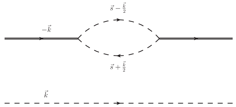
In Fig. 3, all relevant momenta are shown explicitly for the self-energy correction of the $f_{0}(980)$ or the $a_{0}(980)$ meson in TOPT.

The expression corresponding to Fig. 3 may be written in the following form

where $s_{\pm}=s\pm k/2$. Since in this exploratory study the inelasticities of the $a_{0}(980)$ and $f_{0}(980)$ are neglected, both states appear as stable bound states. To ensure that the amplitudes generate the $a_{0}(980)/f_{0}(980)K$ branch cuts correctly, instead of Eq. (17) in the three-body equations we need to employ a renormalized self-energy as shown in Hanhart:2010wh and A

where

Note that this procedure needs to be generalized when inelastic channels [for our example $\pi\pi$ for the $f_{0}(980)$ and $\pi\eta$ for the $a_{0}(980)$] are switched on, since the mentioned cut does not disappear, but moves into the complex plane of the unphysical sheet Doring:2009yv, with the location of the corresponding branch point being related to the complex pole position of the resonance involved.

The expression of the self-energy as defined in Eq. (17) contains both $k$ and $E$ in a non-trivial way. In case of non-relativistic kinematics, one finds

where the $k^{2}$ term captures the kinetic energy of the two-kaon system in the overall center-of-mass frame. With this, the $k$ and $E$ dependence of the self-energy can be absorbed into an effective energy

and the self-energy depends on this single variable only. However, for relativistic kinematics this appears to be not possible and both the $k$ and the $E$ dependence need to be kept explicitly. While $k\ll m_{K}$ and $s\ll m_{K}$ might be a good approximation for the system studied here in the absence of inelastic channels, it is certainly invalid as soon as the $\pi\pi$ and $\pi\eta$ channels are included. Because of this and the reason presented in the introduction, we proceed using relativistic kinematics. Note that, to speed up the numerical solution of the integral equation, the self-energy can be calculated for the energies of interest outside the routine that fills the potential directly on the grid employed for the discretisation of the integral in the LS equation.

To render the LS equation in Eq. (3) well defined, it is regularized by a finite momentum cutoff $\Lambda$. For consistency the same cutoff is employed for the self-energy defined in Eq. (18), although the regularized expression is formally convergent. In our calculation, we vary the value of $\Lambda$ in the range from 0.5 GeV to 2.0 GeV. To illustrate the resulting cutoff dependence of $f_{S}^{2}\Sigma_{R}(E,k)$, the numerical results corresponding to $E=1.474$ GeV are shown in Fig. 4.

From the condition that the residue of the renormalized propagator $G_{r}(E,k)$ in Eq. (3) is one at

we get

The derivation of this expression is presented in A. The physical value of $f_{S}$ is fixed to be 3.74 GeV. The values of $Z$ corresponding calculated in this way are quoted in Tab. 2. In addition we show their energy dependence for $\Lambda=1$ GeV and 2 GeV in Fig. 5. Thus we find a negligible energy dependence of the $Z$ factor as it should be in general, however, this feature could have been distorted here by the non-covariance of the formalism.

Most of the integrals entering the LS equation are formally convergent. Only those that contain the $s$–channel diagrams lead to a divergence and correspondingly may lead to a sizeable regulator dependence. However, at least the divergence in the one particle reducible diagrams introduced via the kaon pole diagram can be absorbed into mass and wave function regularization. In this procedure the bare parameters $f_{1}^{(0)}$, $f_{2}^{(0)}$ and $m_{K}^{(0)}$, introduced in Eq. (13), are determined from

and

with

and

Here we used the short hand notation $\Gamma_{\lambda^{\prime}\lambda}=\Gamma_{\lambda^{\prime}\lambda}(m_{K},0)$ and $\Sigma_{\lambda^{\prime}\lambda}^{(3)}=\Sigma_{\lambda^{\prime}\lambda}^{(3)}(m_{K})$. Explicit expressions for the self energy of the kaon pole and the dressed vertex function as well as the derivation of Eq. (23) and Eq. (24) are presented in B.

The solution of the LS equation is found by straightforward numerical matrix inversion. For this we use the method given in Ref. Haftel:1970zz. In our calculation, a 40-point Gaussian quadrature yields stable results. Note that since we only study energies below the $a_{0}/f_{0}K$ threshold, no three-body singularities need to be dealt with numerically.

The requirement that Eq. (3) has a pole at some energy $E$ is equivalent to the condition

For a given pole the binding energy is $E_{B}=m^{(1)}+m_{K}-E$, since we measure the energy relative to the $f_{0}(980)K$ threshold (which for the parameters employed here equals to the $a_{0}(980)K$ threshold).

For our study all parameters are fixed as discussed above, however, we still quote the bare, calculated parameters for the single and the coupled channel calculation in Tab. 3 to illustrate that the renormalization effects can in fact be quite sizeable. Moreover, note that for the coupled channel case, although the dressed couplings of $a_{0}(980)$ and $f_{0}(980)$ to kaon-antikaon are equal, the corresponding bare couplings are different due to the different isospin factors in the different channels.

We start the discussion by omitting the effect of the self-energy $\Sigma_{R}^{(\lambda)}(E,k)$ in Eq. (3) by setting $\alpha=0$ and $Z=1$. In this case the three-body scattering generates a bound state pole very close to the threshold on the physical sheet as soon as we study the coupled-channel $Kf_{0}(980)$-$Ka_{0}(980)$ formalism is used — the corresponding binding energies that arise when more and more terms are added to the potential are shown by the columns $f(a)-s(b)$ in the lines marked by $\alpha=0$ in Tab. 4 and as the first four green bars in Fig. 6, where the relative importance of the different contributions calculated for $\Lambda=1$ GeV is illustrated. For the single-channel $Kf_{0}(980)$ formalism, the three-body scattering does not generate a bound state, reflecting that the coupled-channel effect has a strong influence on the scattering process. Here, we employed $f_{S}=3.74$ GeV, fixed via Eq. (3) by the masses of $f_{0}(980)$ and $a_{0}(980)$.

The dependence of the resulting binding energy on the four different cut-offs for the coupled channel case is also shown in Table 4. Clearly for the contributions discussed so far the cut-off dependence is rather weak. Although not directly reflected in the numbers reported in the table, it turns out that the most dominant contribution to the emergence of the bound state comes from the first diagram of the $t$-channel kaon exchange labled as $t(a)$: When using only individual contributions in solving the LS equation, only this part of the potential generates binding. This is expected, since this contribution contains the leading three-body singularity. The second $t$-channel contribution, although not binding by itself, is still important quantitatively as it increases the binding energy by about 30%. Also the two $s$-channel contributions are large individually, however, there are quite effective cancellations among $t(b)$, $s(a)$ and $s(b)$ such that the binding energy deduced from the full potential to order $f_{S}^{2}$ for all cut-offs is within 2% of the one calculated from $t(a)$ only ($cf.$ the sixth column of Tab. 4).

Since both $f_{0}(980)$ and $a_{0}(980)$ couple strongly to the $K\bar{K}$ system, the implications of three-body unitarity above the three kaon-threshold and its impact on analyticity should play an important role in the three-body dynamics. We thus repeat the calculation with $\alpha=1$ and the values of $Z$ given in Fig. 5. As expected the binding energies calculated for the four different cut-offs become lager by more than a factor of 3, see the lines marked with $\alpha=1$ in Tab. 4. Moreover, also the relative contributions from the individual other diagrams get enhanced (e.g. when diagram $t(b)$ is added the binding energy get enhanced by almost a factor of 2; the contributions from the $s$-channel diagrams are even larger). Also the cut-off dependence is now larger. However, the binding energies deduced from the sum of the full potential to order $f_{S}^{2}$ remains very close to that calculated from $t(a)$ only as shown by the numbers in bold face in the sixth column of Tab. 4 as well as the fourth bar in Fig. 6.

Thus, our numerical results suggest that a $I(J^{P})=\frac{1}{2}(0^{-})$ bound state can be generated from from coupled-channel $Kf_{0}(980)$-$Ka_{0}(980)$ interactions, at least as long as inelastic channels are omitted. The binding energies deduced from the interactions discussed so far are below 2 MeV. We also show that for reliable quantitative results the full potential to order $f_{S}^{2}$ needs to be included, since the individual pieces of the potential undergo significant cancellations.

The potentials introduced in Sec. 2 have only physical singularities, but are not invariant under Lorentz transformations. In this section we investigate how much the results change when also the contributions of the streched boxes are included in the potential that restore covariance at the one-loop level. We demonstrate below that their effect on the results is rather small — in any case of the same order a other contributions to the potential higher order in the couplings $f_{S}$.

To show how the violation of covariance emerges in time–ordered perturbation theory, we start from the expression for the t-channel potential given in Eq. (10). The two terms can be combined to

where

is the average off-shellness of the initial and final state for any give pair of momenta $p$ and $p^{\prime}$ and

denotes the energy transfer for initial and final particles on their mass shell. For both particles entering and leaving the potential being on the energy shell, $E^{\rm off}$ vanishes and the potential reduces to the well known, covariant Feynman amplitude

where $t$ is the four-momentum transfer squared, as it should be. However, when being put into the LS equation, both $p$ and $p^{\prime}$ are integration variables and thus the potential is typically evaluated off-shell. Then clearly there is a difference between the two potentials. To keep covariance also then, the formalism of Ref. Mai:2017vot calls for putting Eq. (30) into an LS type equation. This keeps formal covariance, however, it introduces unphysical singularities Dawid:2020uhn. We propose to use the full potential of Eq. (29) or equivalently Eq. (10) instead. This avoids unphysical singularities, but violates covariance, since the potential depends on the particle energies which are not invariant under Lorentz transformations.

To quantify the amount of violation of Lorentz invariance, we calculate explicitly the contributions that restore it at the one loop level. This is achieved by the inclusion of the so-called streched boxes. The corresponding diagrams are shown in Figs. 7, 8, 9 and 10, the related amplitudes are given in Eqs. (C) to (C) in the appendix. The effect of the inclusion of these diagrams into the potential on the resulting binding energies for the different calculations is illustrated by the second to last column in Table 4. The streched boxes change the binding energies in all calculations by about 20% and we may regard this as a subleading contribution. It should be noted that to restore covariance also at the two-loop level higher streched boxes (contributing at order $f_{S}^{6}$) would need to be included. Those are even more suppressed kinematically than the ones at order $f_{S}^{4}$, since more particles are included in the equal time slices. We therefore conclude that the violation of Lorentz invariance for the equations employed here is in the energy range studied indeed mild and can be restored in a controlled way. In contrast to this introducing the mentioned unphysical singularities generates an error in the calculation that cannot be controlled quantitatively.

Moreover, there are additional diagrams at order $f_{S}^{4}$ that turn out to be of the same size as the streched boxes, but are of a different topology. Those are the crossed boxes as shown in Figs. 11, 12, 13 and 14. The related amplitudes are given in Eqs. (C) to (C) in the appendix. The effect of the mentioned contributions can again be read off from the last column of Table 4. It appears therefore not appropriate to employ a formalism where the covariance of the ladder type diagrams is enforced but diagrams of the crossed box type are ignored.

The final contribution necessary to restore covariance at the one-loop level is an additional one loop-correction to the self-energy of the scalar mesons. The corresponding diagram is shown in Fig. 15. Since this contribution is not an addition to the scattering potential, but modifies the $f_{0}(980)/a_{0}(980)K$ propagator in the LS equation, it also modifies the binding energies calculated from the scattering potential to order $f_{S}^{2}$. Therefore we report its effect by additional lines in Table 4. Those are labeled with $\alpha=1^{\dagger}$. The effect of this contribution is a moderate reduction of the calculated binding energies, however, the effect is no larger than the one of the crossed boxes. This can be traced to the fact that the energy dependence of the resulting self energy-contribution is quite weak and thus the threshold subtraction to renormalize the self energy largely removes the contribution of the second time ordering.

It should be noted that the final results now including the restoration of the covariance to one loop shows a larger dependence of the regulator than the one without those corrections. The reason for this is most probably that the added terms contain in the time slices more of the heavier scalar fields that introduce larger momentum scales into the integrals. This observation indicates that a proper renormalization to this order might require a three-kaon counter term. However, addressing this issue, which calls for a proper power counting of the system, goes beyond the scope of this paper.

In this work we provide additional support for the proposal put forward in Ref. Epelbaum:2016ffd to employ time ordered perturbation theory with relativistic particle energies in calculations of three-body scattering. To be concrete we demonstrate on the example of isospin $1/2$ three-body $KK\bar{K}$ scattering in the isobar formalism that the effect of the violation of covariance on the binding energies for three-body bound states is rather mild and can even be removed in a systematic way by inclusion of the streched boxes, although a restoration of covariance at the two-loop level in practice would be a formidable task given the large number of time orderings that would need to be included. Moreover, we demonstrate in addition that the so-called crossed box contributions are of similar importance than the streched boxes. This shows that a systematic calculation of three-body bound states using time ordered perturbation theory could be set up by including at leading order just the contributions to the potential at order $f_{S}^{2}$, at next-to-leading order the two-particle irreducible contributions (here two-particle refers for the concrete example studied here to an intermediate state of an isobar and a kaon) at order $f_{S}^{4}$ and so on, where the latter group should not only contain the new topologies that appear at this order but also the diagrams that restore covariance at the one loop level. All two-particle reducible contributions are enhanced kinematically and are automatically generated via the LS equation. Our results suggest that the binding energies of the three kaon system can be well estimated by including the contribution from $t(a)$ only in the potential, although this violates covariance.

This kind of procedure avoids the need to use covariant potentials in a three dimensional formalism that can introduce unphysical singularities Mai:2017vot; Dawid:2020uhn or to solve the very complicated four-dimensional scattering equations Phillips:1996ed; Lahiff:2002wp. Clearly, a further improved calculation needs to consider the contribution from inelastic channels as well as the Goldstone boson nature of the participating particles.

References

• (1) P. A. Zyla et al. [Particle Data Group], PTEP 2020 (2020) no.8, 083C01.
• (2) F. K. Guo, X. H. Liu and S. Sakai, Prog. Part. Nucl. Phys. 112 (2020) 103757 [arXiv:1912.07030 [hep-ph]].
• (3) Y. R. Liu et al., Prog. Part. Nucl. Phys. 107 (2019) 237 [arXiv:1903.11976 [hep-ph]].
• (4) F. K. Guo et al., Rev. Mod. Phys. 90 (2018) no.1, 015004 [arXiv:1705.00141 [hep-ph]].
• (5) H. X. Chen et al., Rept. Prog. Phys. 80 (2017) no.7, 076201 [arXiv:1609.08928 [hep-ph]].
• (6) N. Brambilla et al., Phys. Rept. 873 (2020), 1-154 [arXiv:1907.07583 [hep-ex]].
• (7) K. P. Khemchandani, A. Martinez Torres and E. Oset, Eur. Phys. J. A 37 (2008) 233 [arXiv:0804.4670 [nucl-th]].
• (8) D. L. Canham, H. W. Hammer and R. P. Springer, Phys. Rev. D 80 (2009), 014009 [arXiv:0906.1263 [hep-ph]].
• (9) V. Baru, A. A. Filin, C. Hanhart, Y. S. Kalashnikova, A. E. Kudryavtsev and A. V. Nefediev, Phys. Rev. D 84, 074029 (2011) [arXiv:1108.5644 [hep-ph]].
• (10) L. Ma, Q. Wang and U.-G. Meißner, Chin. Phys. C 43, no.1, 014102 (2019) [arXiv:1711.06143 [hep-ph]].
• (11) Q. Wang, V. Baru, A. A. Filin, C. Hanhart, A. V. Nefediev and J. L. Wynen, Phys. Rev. D 98, no.7, 074023 (2018) doi:10.1103/PhysRevD.98.074023 [arXiv:1805.07453 [hep-ph]].
• (12) T. W. Wu, M. Z. Liu, L. S. Geng, E. Hiyama and M. P. Valderrama, Phys. Rev. D 100 (2019) no.3, 034029 [arXiv:1906.11995 [hep-ph]].
• (13) Walter Glöckle, The Quantum Mechanical Few-Body Problem, Springer, Berlin, Heidelberg, New York Tokyo, 1983.
• (14) A. A. Filin et al., Phys. Rev. Lett. 105 (2010), 019101 doi:10.1103/PhysRevLett.105.019101 [arXiv:1004.4789 [hep-ph]].
• (15) E. Epelbaum, J. Gegelia, U. G. Meißner and D. L. Yao, Eur. Phys. J. A 53, no.5, 98 (2017) doi:10.1140/epja/i2017-12288-3 [arXiv:1611.06040 [nucl-th]].
• (16) V. N. Efimov, Sov. J. Nucl. Phys. 12, 589 (1971).
• (17) P. F. Bedaque, H. W. Hammer and U. van Kolck, Phys. Rev. Lett. 82, 463-467 (1999) [arXiv:nucl-th/9809025 [nucl-th]].
• (18) F. E. Close, N. Isgur and S. Kumano, Nucl. Phys. B 389 (1993) 513 [hep-ph/9301253].
• (19) J. A. Oller and E. Oset, Nucl. Phys. A 620 (1997) 438 Erratum: [Nucl. Phys. A 652 (1999) 407] [hep-ph/9702314].
• (20) J. Nieves and E. Ruiz Arriola, Nucl. Phys. A 679 (2000) 57 [hep-ph/9907469].
• (21) V. Baru et al., Phys. Lett. B 586 (2004) 53 [hep-ph/0308129].
• (22) J. R. Pelaez, Phys. Rev. Lett. 92 (2004) 102001 [hep-ph/0309292].
• (23) Y. S. Kalashnikova et al., Eur. Phys. J. A 24 (2005) 437 [hep-ph/0412340].
• (24) N. N. Achasov and A. V. Kiselev, Phys. Rev. D 73 (2006) 054029 Erratum: [Phys. Rev. D 74 (2006) 059902] [hep-ph/0512047].
• (25) F. Ambrosino et al. [KLOE Collaboration], Eur. Phys. J. C 49 (2007) 473 [hep-ex/0609009].
• (26) S. Weinberg, Phys. Rev. 130 (1963), 776-783.
• (27) I. Matuschek, V. Baru, F. K. Guo and C. Hanhart, Eur. Phys. J. A 57 (2021) no.3, 101 [arXiv:2007.05329 [hep-ph]].
• (28) C. Hanhart et al., Phys. Rev. D 75 (2007) 074015 [hep-ph/0701214].
• (29) M. Ablikim et al. [BESIII], Phys. Rev. Lett. 121 (2018) no.2, 022001 [arXiv:1802.00583 [hep-ex]].
• (30) C. Hanhart, B. Kubis and J. R. Pelaez, Phys. Rev. D 76 (2007), 074028 [arXiv:0707.0262 [hep-ph]].
• (31) J. J. Wu and B. S. Zou, Phys. Rev. D 78 (2008), 074017 [arXiv:0808.2683 [hep-ph]].
• (32) L. Roca, Phys. Rev. D 88 (2013), 014045 [arXiv:1210.4742 [hep-ph]].
• (33) G. W. Brandenburg et al., Phys. Rev. Lett. 36 (1976) 1239.
• (34) C. Daum et al. [ACCMOR Collaboration], Nucl. Phys. B 187 (1981) 1.
• (35) R. Aaij et al. [LHCb Collaboration], Eur. Phys. J. C 78 (2018) no.6, 443 [arXiv:1712.08609 [hep-ex]].
• (36) M. Albaladejo, J. A. Oller and L. Roca, Phys. Rev. D 82 (2010) 094019 [arXiv:1011.1434 [hep-ph]].
• (37) A. Martinez Torres, D. Jido and Y. Kanada-En’yo, Phys. Rev. C 83 (2011) 065205 [arXiv:1102.1505 [nucl-th]].
• (38) I. Filikhin et al., arXiv:2008.00111 [nucl-th].
• (39) R. S. Longacre, Phys. Rev. D 42 (1990) 874.
• (40) S. Godfrey and N. Isgur, Phys. Rev. D 32 (1985) 189.
• (41) R. Aaron, R. D. Amado and J. E. Young, Phys. Rev. 174 (1968) 2022.
• (42) M. Mai et al., Eur. Phys. J. A 53 (2017) no.9, 177 [arXiv:1706.06118 [nucl-th]].
• (43) G. Janssen, K. Holinde and J. Speth, Phys. Rev. C 49 (1994) 2763.
• (44) D. Sadasivan et al., Phys. Rev. D 101 (2020) no.9, 094018 [arXiv:2002.12431 [nucl-th]].
• (45) A. Jackura et al. [JPAC Collaboration], Eur. Phys. J. C 79, no. 1, 56 (2019) [arXiv:1809.10523 [hep-ph]].
• (46) N. N. Khuri and S. B. Treiman, Phys. Rev. 119, 1115-1121 (1960).
• (47) F. Niecknig, B. Kubis and S. P. Schneider, Eur. Phys. J. C 72, 2014 (2012) [arXiv:1203.2501 [hep-ph]].
• (48) F. Niecknig and B. Kubis, JHEP 10, 142 (2015) doi:10.1007/JHEP10(2015)142 [arXiv:1509.03188 [hep-ph]].
• (49) F. Niecknig and B. Kubis, Phys. Lett. B 780, 471-478 (2018) [arXiv:1708.00446 [hep-ph]].
• (50) T. Isken, B. Kubis, S. P. Schneider and P. Stoffer, Eur. Phys. J. C 77, no.7, 489 (2017) [arXiv:1705.04339 [hep-ph]].
• (51) J. Gasser and A. Rusetsky, Eur. Phys. J. C 78, no.11, 906 (2018) doi:10.1140/epjc/s10052-018-6378-8 [arXiv:1809.06399 [hep-ph]].
• (52) M. Albaladejo et al. [JPAC], Phys. Rev. D 101, no.5, 054018 (2020) [arXiv:1910.03107 [hep-ph]].
• (53) M. Albaladejo et al. [JPAC], Eur. Phys. J. C 80, no.12, 1107 (2020) [arXiv:2006.01058 [hep-ph]].
• (54) S. M. Dawid and A. P. Szczepaniak, Phys. Rev. D 103, no.1, 014009 (2021) doi:10.1103/PhysRevD.103.014009 [arXiv:2010.08084 [nucl-th]].
• (55) D. Lohse et al., Nucl. Phys. A 516 (1990) 513.
• (56) D. Gülmez, U.-G. Meißner and J. A. Oller, Eur. Phys. J. C 77 (2017) no.7, 460 [arXiv:1611.00168 [hep-ph]].
• (57) C. Hanhart, Y. S. Kalashnikova and A. V. Nefediev, Phys. Rev. D 81 (2010) 094028 [arXiv:1002.4097 [hep-ph]].
• (58) M. Döring et al., Nucl. Phys. A 829 (2009), 170-209 [arXiv:0903.4337 [nucl-th]].
• (59) M. I. Haftel and F. Tabakin, Nucl. Phys. A 158 (1970) 1.
• (60) O. Krehl, C. Hanhart, S. Krewald and J. Speth, Phys. Rev. C 62 (2000), 025207 doi:10.1103/PhysRevC.62.025207 [arXiv:nucl-th/9911080 [nucl-th]].
• (61) D. R. Phillips and I. R. Afnan, Phys. Rev. C 54, 1542-1560 (1996) [erratum: Phys. Rev. C 55, 3178 (1997)] doi:10.1103/PhysRevC.55.3178 [arXiv:nucl-th/9605004 [nucl-th]].
• (62) A. D. Lahiff and I. R. Afnan, Phys. Rev. C 66, 044001 (2002) doi:10.1103/PhysRevC.66.044001 [arXiv:nucl-th/0205076 [nucl-th]].