Efficient Reduced Basis Algorithm (ERBA) for kernel-based approximation

We introduce the kernel-based scattered data interpolation problem following [7, 15]. Let $\Omega\subseteq\mathbb{R}^{d}$ and ${\cal X}=\{\bm{x}_{i},\;i=1,\ldots,n\}\subset\Omega$ be a set of distinct nodes, $n\in\mathbb{N}$, where $\bm{x}_{i}=(x_{i,1},\dots,x_{i,d})^{\intercal}$, $i=1,\dots,n$. The scattered data interpolation problem consists in recovering an unknown function $f\mathrel{\mathop{\mathchar 58\relax}}\Omega\longrightarrow\mathbb{R}$ given its values at ${\cal X}$, i.e. $\bm{f}=\bm{f}_{|{\cal X}}=(f(\bm{x}_{1}),\dots,f(\bm{x}_{n}))^{\intercal}=(f_{1},\dots,f_{n})^{\intercal}$. This can be achieved by imposing the interpolation conditions at ${\cal X}$. In particular, for kernel-based interpolation, the approximating function assumes the form:

where $\bm{c}=(c_{1},\dots,c_{n})^{\intercal}\in\mathbb{R}^{n}$ and $\kappa_{\varepsilon}\mathrel{\mathop{\mathchar 58\relax}}\Omega\times\Omega\longrightarrow\mathbb{R}$ is a strictly positive definite kernel depending on a shape parameter $\varepsilon>0$. In addition, $\kappa_{\varepsilon}$ is supposed to be radial, i.e. there exists a univariate function $\varphi_{\varepsilon}\mathrel{\mathop{\mathchar 58\relax}}\mathbb{R}_{\geq 0}\longrightarrow\mathbb{R}$ such that $\kappa_{\varepsilon}(\bm{x},\bm{y})=\varphi_{\varepsilon}(r)$, with $r\coloneqq\lVert\bm{x}-\bm{y}\lVert_{2}$, where $\lVert\cdot\lVert_{2}$ is the Euclidean norm. As a consequence, such a setting is commonly referred to as Radial Basis Function (RBF) interpolation. Clarified this and with abuse of notation, we might write simply $\kappa$ instead of $\kappa_{\varepsilon}$. The interpolation conditions are satisfied by finding the unique vector $\bm{c}$ so that

where $\mathsf{A}=(\mathsf{A}_{i,j})=\kappa(\bm{x}_{i},\bm{x}_{j})$, $i,j=1,\dots,n$, is the so-called interpolation (or collocation or simply kernel) matrix. The uniqueness of the solution of (1) is guaranteed as long as $\kappa$ is strictly positive definite. For a more general formulation of the interpolant that involves conditionally positive definite kernels, and for a complete overview concerning kernel-based approximation, we refer the reader e.g. to [15].

The interpolant $S_{f,\mathcal{X}}$ belongs to the space

which equipped with the bilinear form $(\cdot,\cdot)_{\mathcal{H}_{\kappa}}$ is a pre-Hilbert space with reproducing kernel $\kappa$. Moreover, the completion of $\mathcal{H}_{\kappa}$ with respect to the norm $\lVert\cdot\lVert_{\mathcal{H}_{\kappa}}=\sqrt{(\cdot,\cdot)_{\mathcal{H}_{\kappa}}}$ is the so-called native space $\mathcal{N}_{\kappa}$ associated to $\kappa$. Many upper bounds for the interpolation error, e.g. in terms of the fill-distance [7, Theorem 14.5, p. 121] and using sampling inequalities [9, 14], are available. Here we focus on the following pointwise error bound [7, Theorem 14.2, p. 117]:

where $P_{\kappa,\mathcal{X}}$ is the so-called power function. For our scopes, we directly define the power function as [8, p. 116, §14]:

where

Note that (2) splits the error into two terms. The former, i.e. the power function, only depends on the nodes and on the kernel, while the latter takes into account the function values.

As a consequence, the power function gives information about how the interpolation error relates to the node distributions. Indeed, as for polynomial and spline interpolation, the approximation quality strongly depends on the distribution of the scattered data. In view of this, possibly starting from an initial set of nodes, many adaptive strategies have been studied in order to construct well-behaved interpolation designs, i.e. interpolation sets which provide an accurate reconstruction and, preferably, affordable computational costs. In particular, the so-called greedy approaches match such purposes by iteratively adding new points to the interpolation set. The iterative rule is based on minimizing a pointwise upper bound for the interpolant. Precisely, those strategies rely on the residual of the interpolant ($f$-greedy) or on the value of the power function ($p$-greedy); refer to [5, 10, 17, 18, 19] for a general overview. These methods fall under the context of knot insertion algorithms, which have been studied also in the context of adaptive least-squares approximation [7, §21].

Alternatively, as in our work, one could start by taking a large interpolation set, which provides an accurate approximation, and iteratively remove nodes until the resulting interpolation error does not exceed a fixed tolerance (see e.g. [11] for a general overview). This kind of knot removal approaches aim to provide reduced models by neglecting as many points as possible from the initial set while preserving a target accuracy. However, they are usually computationally expensive, since many interpolants built upon large sets of nodes need to be constructed [6].

In this paper, in order to overcome the limitations related to the high computational complexity for reduced basis models, we take advantage of the extension of the Rippa’s algorithm [13] recently provided in [12]. More precisely, we propose the Efficient Reduced Basis Algorithm (ERBA) where the Extended Rippa’s Algorithm (ERA) plays a fundamental role. Besides the residual-based rule, that leads to the ERBA-$r$, and that can be derived from the ERA, we provide an efficient scheme for computing the power function as well. The resulting ERBA-$p$ is a reduced model that takes advantage of being accurate, fast and easy to implement.

The paper is organised as follows. In Section 2, we fix some notations and we introduce the Reduced Basis Algorithm (RBA) based on knot removal strategies. Its efficient implementation, i.e. the ERBA scheme, and theoretical results are then provided in Section 3, where a detailed analysis of the computational complexity of the proposed schemes is also included. Numerical tests that confirm the theoretical findings are presented in Section 4. The conclusions are offered in Section 5.

In what follows, we present our schemes for reduced basis models based on both the residual and on the power function minimization. The latter algorithm is quasi optimal in the sense that, referring to (2), we only take into account the power function, neglecting the term involving the native space norm of the sought function. This should not be seen as a drawback. Indeed, we are able to compute a quasi-optimal subset of points independently of the function values. As a consequence, it might be relevant if one has to deal with many measurements sampled at the same points. We further point out that the residual-based scheme shows strong similarities with the knot removal algorithm presented in [7, §21]. We now present the RBA scheme and in the next section we focus on its fast implementation.

Given ${\cal X}=\{\bm{x}_{i},\;i=1,\ldots,n\}\subset\Omega$ be the initial set of nodes and ${\cal X}_{s-1}=\{\bm{x}_{i},\;i=1,\ldots,n_{s-1}\}\subset\Omega$ be the reduced set at the $(s-1)$-th step of the algorithm (${\cal X}_{0}={\cal X}$), let $\tau\in\mathbb{R}_{>0}$ be a fixed tolerance. Chosen $\rho\in\mathbb{N}$, $\rho<n$, and letting $\ell=\lfloor n_{s-1}/\rho\rfloor$, the $s$-th step of the iterative scheme, $s\geq 1$, is as follows.

1. 1.

   Partition $\mathcal{X}_{s-1}$ into $\ell$ test sets $\mathcal{X}_{s-1}^{1},\dots,\mathcal{X}_{s-1}^{\ell}$, $|\mathcal{X}_{s-1}^{j}|=\rho^{j}$ with $\rho^{j}\in\{\rho,\dots,2\rho\}$. Moreover, let $\overline{\mathcal{X}}_{s-1}^{j}\coloneqq\mathcal{X}_{s-1}\setminus\mathcal{X}_{s-1}^{j}$ be the training sets, $j=1,\ldots,\ell$.

2. 2.

   For each $\mathcal{X}_{s-1}^{j}$, $j=1,\dots,\ell$, compute:

   • 2a.

     in the case of the residual-based scheme:

     $$w^{j}=\dfrac{1}{\sqrt{\rho^{j}}}\lVert\bm{f}^{j}-\bm{S}^{j}\lVert_{2},$$

     (3)

     where $\bm{f}^{j}\coloneqq\bm{f}_{|_{\mathcal{X}_{s-1}^{j}}}$ and $\bm{S}^{j}\coloneqq S_{f,\overline{\mathcal{X}}_{s-1}^{j}}(\mathcal{X}_{s-1}^{j})$ is the evaluation vector on $\mathcal{X}_{s-1}^{j}$ of the interpolant $S_{f,\overline{\mathcal{X}}_{s-1}^{j}}$;

   • 2b.

     in the case of the power-based scheme:

     $$w^{j}=\dfrac{1}{\sqrt{\rho^{j}}}\lVert\bm{P}^{j}\lVert_{2},$$

     where $\bm{P}^{j}\coloneqq P_{\kappa,\overline{\mathcal{X}}_{s-1}^{j}}(\mathcal{X}_{s-1}^{j})$ is the evaluation vector on $\mathcal{X}_{s-1}^{j}$ of the power function $P_{\kappa,\overline{\mathcal{X}}_{s-1}^{j}}$.

3. 3.

   Choose

   $$j^{\star}=\argmin_{j\in\{1,\dots,\ell\}}{w^{j}}.$$

4. 4.

   Let $r_{s-1}=w^{j^{\star}}$:

   • 4a.

     if $r_{s-1}\leq\tau$, define $\mathcal{X}_{s}=\mathcal{X}_{s-1}\setminus\mathcal{X}_{s-1}^{j^{\star}}$ and proceed iteratively with the $s$-th step;

   • 4b.

     if $r_{s-1}>\tau$, $\mathcal{X}_{s}=\mathcal{X}_{s-1}$ is the final interpolation set obtained by the procedure.

The convergence of the residual-based scheme has been studied in many context and for many basis functions, see e.g. [11] for a general overview. As far as the convergence of the proposed error-based scheme is concerned, it is ensured by the fact that [10, Lemma 5]:

being $V(\mathcal{X}_{s})\subset V(\mathcal{X}_{s-1}),$ linear subspaces of the nested sets $\mathcal{X}_{s}$ and $\mathcal{X}_{s-1}$.

From now on, in analyzing the computational complexity, we assume without loss of generality that $\rho$ divides $n_{s}$ at each step of the algorithm, and thus $\rho_{j}\equiv\rho$ holds true. Therefore, at each step, a classical implementation of this method requires to solving $n_{s}$ different $(n_{s}-\rho)\times(n_{s}-\rho)$ linear systems, in the residual-based case, or the inversion of a $(n_{s}-\rho)\times(n_{s}-\rho)$ matrix in the power-based setting. Hence, in both situations, each step is computationally demanding. In [7, §21], a similar residual-based approach has been speeded up by using Rippa’s algorithm in the case $\rho=1$. In the next section, inspired by ERA [12] we provide a fast implementation of the proposed algorithm.

To study the computational complexity of the proposed schemes, we have to focus on the calculation of the residuals (or of the power function) that is performed at each step. Then, fixed a certain iteration $s=1,2,\dots$, let us introduce the following notations: $\mathcal{X}_{s}\coloneqq\mathcal{X}$, $n_{s}\coloneqq n$, and let $\bm{p}\coloneqq(p_{1},\dots,p_{\rho})^{\intercal}$ be the vector of $\rho$ indices related to the elements of the subset $\mathcal{X}_{s}^{j}\coloneqq\mathcal{V}$, $|\mathcal{X}_{s}^{j}|=\rho$. We also adopt the following notations:

In the following we explain our efficient strategy for the implementation of both the residual and power-based schemes.

In what follows, we perform some numerical experiments to prove the efficiency of the proposed ERBA. The tests have been carried out in Matlab on a Intel(R) Core(TM) i7-1165G7 CPU@2.80GHz processor. The software is available for the scientific community at

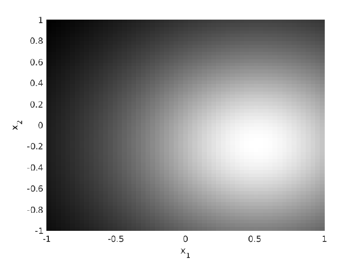
Let $\Omega=[-1,1]^{2}$ and let $f\mathrel{\mathop{\mathchar 58\relax}}\Omega\longrightarrow\mathbb{R}$ be a function defined as

For the tests, we take the strictly positive definite kernel

and we set $\varepsilon=1$.

As interpolation data set $\mathcal{X}\subset\Omega$, we consider a $n\times n$ grid, with $n=25$. Moreover, we take a $m\times m$ evaluation grid $\Xi$ with $m=60$. The associated RMSE computed on $\Xi$ is $e_{\mathcal{X}}=9.69{\rm E}-05$. In Figure 1, we plot the function $f$ and the interpolant $S_{f,\mathcal{X}}$ evaluated on $\Xi$.

We have investigated a fast computation of a knot removal scheme. We have implemented two different strategies: the first one in based on classical residual-based schemes while the second one relies on power function error bounds. The latter is independent on the function values and tends to return quasi-uniform data (cf. [4] and [16, Theorem 15 & 19 & 20]), while the former, as expected, keeps points where the corresponding function has steep gradients. In both cases we are able to significantly speed up the algorithm thanks to our implementation.

Work in progress consists in extending the proposed tool to other bases, e.g. splines [1] and to variably scaled kernels [2]. Moreover, it can be helpful for validating the shape parameter in RBF interpolation; refer e.g. to [3].

This research has been accomplished within Rete ITaliana di Approssimazione (RITA) and the UMI Group TAA Approximation Theory and Applications; partially funded by GNCS-IN$\delta$AM and by the ASI - INAF grant “Artificial Intelligence for the analysis of solar FLARES data (AI-FLARES)”.

References

- [1] R. Campagna, C. Conti, S. Cuomo, Smoothing exponential-polynomial splines for multiexponential decay data, Dolomites Res. Notes Approx. 12 (2018), pp. 86–100.
- [2] C. Campi, F. Marchetti, E. Perracchione, Learning via variably scaled kernels, Adv. Comput. Math. 47 (2021), 51.
- [3] R. Cavoretto, A. De Rossi, M.S. Mukhametzhanov, Y.D. Sergeyev, On the search of the shape parameter in radial basis functions using univariate global optimization methods, J. Glob. Optim. 79 (2021), 305–327.
- [4] S. De Marchi, R. Schaback, H. Wendland, Near-optimal data-independent point locations for radial basis function interpolation, Adv. Comput. Math. 23 (2005), pp. 317–330.
- [5] S. Dutta, M.W. Farthing E. Perracchione, G. Savant, M. Putti, A greedy non-intrusive reduced order model for shallow water equations, J. Comput. Phys. 439 (2021), 110378.
- [6] G.E. Fasshauer, Adaptive least squares fitting with radial basis functions on the sphere, in: M. Daehlen et al (Eds.), Vanderbilt University Press (Nashville), pp. 141–150.
- [7] G.E. Fasshauer, Meshfree Approximations Methods with Matlab, World Scientific, Singapore, 2007.
- [8] G.E. Fasshauer, M.J. McCourt, Kernel-based Approximation Methods Using Matlab, World Scientific, Singapore, 2015.
- [9] E. Fuselier, G. Wright, Scattered Data Interpolation on Embedded Submanifolds with Restricted Positive Definite Kernels: Sobolev Error Estimates, SIAM J. Numer. Anal. 50, 3 (2012), pp 1753–1776.
- [10] G. Santin, B. Haasdonk, Convergence rate of the data-independent -greedy algorithm in kernel-based approximation, Dolomites Res. Notes Approx. 2 (2017), pp. 68–78.
- [11] T. Lyche, Knot Removal for Spline Curves and Surfaces, in: E.W. Cheney et al (Eds.), Approximation Theory, 1992, pp. 207–226.
- [12] F. Marchetti, The extension of Rippa’s algorithm beyond LOOCV, Appl. Math. Letters, 120 (2021), 107262.
- [13] S. Rippa, An algorithm for selecting a good value for the parameter in radial basis function interpolation, Adv. Comput. Math. 11 (1999), 193–210.
- [14] C. Rieger, Sampling inequalities and applications. Disseration, Göttingen, 2008.
- [15] H. Wendland, Scattered Data Approximation, Cambridge Monogr. Appl. Comput. Math., vol. 17, Cambridge Univ. Press, Cambridge, 2005.
- [16] T. Wenzel, G. Santin, B. Haasdonk, A novel class of stabilized greedy kernel approximation algorithms: Convergence, stability and uniform point distribution, J. Approx. Theory 262 (2021), 105508.
- [17] T. Wenzel, G. Santin, B. Haasdonk, Analysis of target data-dependent greedy kernel algorithms: Convergence rates for -, - and -greedy, ArXiv, 2105.07411 (2021).
- [18] D. Wirtz, N. Karajan, B. Haasdonk, Surrogate modelling of multiscale models using kernel methods, Int. J. Numer. Met. Eng. 101 (2015) pp. 1–28.
- [19] D. Wirtz, B. Haasdonk, A vectorial kernel orthogonal greedy algorithm, Dolomites Res. Notes Approx. 6 (2013) pp. 83–100.