Network meta-analysis and random walksPublication type: Article Type
Abstract
Network meta-analysis (NMA) is a central tool for evidence synthesis in clinical research. The results of an NMA depend critically on the quality of evidence being pooled. In assessing the validity of an NMA, it is therefore important to know the proportion contributions of each direct treatment comparison to each network treatment effect. The construction of proportion contributions is based on the observation that each row of the hat matrix represents a so-called ‘evidence flow network’ for each treatment comparison. However, the existing algorithm used to calculate these values is associated with ambiguity according to the selection of paths. In this work we present a novel analogy between NMA and random walks. We use this analogy to derive closed-form expressions for the proportion contributions. A random walk on a graph is a stochastic process that describes a succession of random ‘hops’ between vertices which are connected by an edge. The weight of an edge relates to the probability that the walker moves along that edge. We use the graph representation of NMA to construct the transition matrix for a random walk on the network of evidence. We show that the net number of times a walker crosses each edge of the network is related to the evidence flow network. By then defining a random walk on the directed evidence flow network, we derive analytically the matrix of proportion contributions. The random-walk approach, in addition to being computationally more efficient, has none of the associated ambiguity of the existing algorithm.
keywords
network meta-analysis, random walks, statistical mechanics, proportion contribution, evidence flow, electrical networks[7]
DAVIES et al
1 Introduction
Network meta-analysis (NMA) has been established as a central tool of evidence synthesis in clinical research[TSD2, DIAS:2018, SALANTI:2012]. Combining direct and indirect evidence from multiple randomised controlled trials, NMA makes it possible to compare interventions that have not been tested together in any trial [Lu:Ades:2004, Hig:White:1996, Lumley:2002]. The term ‘network meta-analysis’ derives from the fact that one can mathematically represent the collection of interventions and trials as a graph. A graph consists of a set of nodes and a set of edges connecting pairs of nodes. The nodes of an NMA graph represent the different treatment options, and edges are comparisons made between the treatments in the trials. In line with Rücker (2012)[Rucker:2012] we will refer to networks of treatment options and comparisons between treatments as ‘meta-analytic graphs’.
An NMA combines data from multiple trials, each comparing different combinations of treatment options. The accuracy of the conclusions from an NMA depends on potential biases associated with individual trials, and on assumptions such as between-trial homogeneity and consistency between direct and indirect evidence. In this context it is useful to study the so-called ‘flow of evidence’ [konig:2013] in the network. This describes the influence different network components have on the estimates of treatment effects. For example, the comparison between two particular treatments may enter as indirect evidence into the estimate of the relative effect of two different nodes in the network. Understanding how exactly evidence flows in the graph then allows one to assess the impact of potential bias originating from different pieces of evidence in the network [konig:2013, Papakon:2018, Nikola:2020].
Previous literature has, for example, looked at the relative influence of direct evidence compared to indirect evidence [Lu:2011, Senn:2012]. Other work has been concerned with measures of network geometry, capturing the frequency with which different comparisons are represented in the trials underpinning an NMA [Salanti:2008, Salanti:2008b]. One then asks how the network structure affects NMA estimates of treatment effects, heterogeneity and rank metrics[Salanti:2008, Salanti:2008b, Davies:2020, Tonin:2019, Veroniki:2018, Kibret:2014]. König et al (2013) [konig:2013] observed that in a two-step (‘aggregate’) NMA model[Lu:2011] each row of the ‘hat matrix’ represents an evidence flow network for a particular treatment effect. König et al then visualised the evidence flow on weighted directed acyclic graphs in which nodes represent treatments, and edges indicate the direction and quantity of evidence flow through each direct comparison. Based on this observation, Papakonstantinou et al (2018) [Papakon:2018] introduced ‘streams’ of evidence and developed a numerical algorithm to calculate these streams. The streams of evidence are then used to derive the ‘proportion contribution’ of each direct comparison to each treatment effect in the graph. This allows one to quantify how limitations of individual studies impact on the estimates obtained from the network. Indeed, the algorithm in Papakonstantinou et al. is implemented in software such as CINeMA (confidence in network meta-analysis) [Nikola:2020] and ROB-MEN (risk-of-bias due to missing evidence in NMA)[Chiocchia:2021], used in clinical practice for the evaluation of results from an NMA.
More widely, the study of networks plays a key role in a variety of disciplines including ecology, economics, electrical engineering and sociology[Mendes:2003, Newman:2018, Estrada:2011]. Through the representation of treatment options and comparisons in trials as a graph, one can therefore take advantage of the extensive literature in network theory, and of ideas developed in the disciplines in which networks are studied. For example one of us [Rucker:2012] used the graph representation of NMA to make the connection between meta-analytic and electrical networks. This allows one to demonstrate that graph theoretical tools routinely applied to electrical networks are also of use in NMA. This approach has since led to advancements in NMA methodology such as frequentist ranking methods [Rucker:2015] and component NMA [Rucker:2020]. It is also the basis for the software package netmeta [netmeta:2021].
In this paper we present a new analogy between random walks and NMA. A random walk on a graph is a stochastic process consisting of a succession of ‘hops’ between vertices connected by edges. Random walks are of interest for a wide range of applications, including statistical physics, biology, ecology, genetics, transport and economics (for a selection of references see [Codling, Okubo, Isichenko, Ewens, Mantegna]). Random walks are also a popular tool to study the properties of networks themselves [Noh:2004, Lov:1994, MASUDA20171].
It is well known that there is a connection between random walks and electrical networks [Kakutani:1945, Kemeny:1966, Kelly:1979, Doyle:2000]. In this context, edges of the electric network are conducting connections (wires). The correspondence between random walks and electrical networks can be established by asserting that the probability that a random walker currently at node moves to node in the next step is proportional to the conductance (inverse resistance) of the edge connecting and . Quantities in the electrical network such as currents along edges or electric potentials at the nodes then have an interpretation in the random-walk picture. For further details we refer to [Doyle:2000].
Motivated by the connection between electrical networks and NMA on the one hand, and that of electrical networks and random walks on the other, we construct a random walk on the meta-analytic network. We show that the random-walk picture we develop can be used to study the flow of evidence in the NMA network. In particular there is a random-walk interpretation of the elements in the hat matrix. Further, we construct a second random-walk model, this time on the evidence flow network. From this we derive an analytical expression for proportion contributions which overcomes the limitations of Papakonstantinou et al [Papakon:2018]. In particular, the algorithm in Papakonstantinou et al selects only a subset of paths on the evidence flow network. This means that paths of evidence that potentially contribute risk of bias are missed. Furthermore, the paths identified by the algorithm are not unambiguous and instead depend on the order in which certain steps are carried out. In contrast, the random-walk approach identifies all possible paths of evidence. The method delivers an unambiguous analytical result for proportion contributions, and less computational effort is required than for the numerical algorithm. In addition, unlike the method in Papakonstantinou et al, the random-walk approach is able to handle networks with multi-arm trials.
The remainder of this paper is set out as follows: We present a motivating data set in Section 2. In Section 3 we provide the relevant background information. We describe an aggregate-level frequentist NMA model and show how the associated hat matrix can be interpreted as evidence flow. In Section 4 we introduce the analogies between NMA, electrical networks and random walks. Using the analogies to electrical networks in both the NMA and random-walk literature, we then express the flow of evidence in an NMA in terms of properties of random walks on the aggregate network. In Section 5 we introduce a second random-walk model, now on the directed evidence flow network. We use this to analytically derive the matrix of proportion contributions. In Section 6, we apply our method to the motivating data set and demonstrate that the random-walk approach overcomes the limitations of the numerical algorithm previously proposed by Papakonstantinou et al (2018) [Papakon:2018]. We summarise our results in Section and discuss potential future impact of the analogy between NMA and random walks.
2 Motivating Example
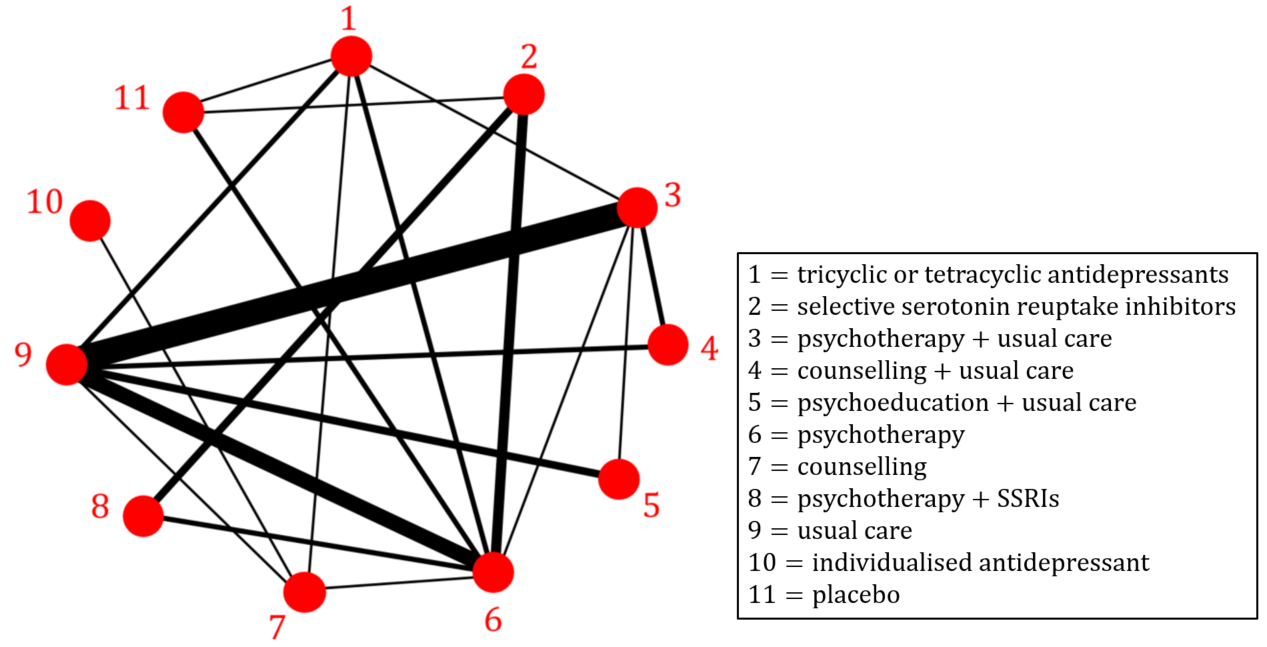
We use an NMA of psychological treatments for patients with depressive disorders [Linde:2013] to motivate our work. The data is described in detail in Rücker and Schwarzer (2014) [Rucker:2014]. For convenience we will occasionally refer to this as the ‘depression data set’. The NMA compares treatments based on randomised controlled trials. Of these one is a four-arm trial, eight are three-arm trials and 17 contain just two arms. In total, the trials provide pairs of treatments which are directly compared in at least one trial. The primary outcome of the trials was a binary variable representing patient response after treatment completion. The odds ratio (OR) was used as the measure of relative treatment effect. The graph representing this set of treatments and trials is shown in Figure 1. Vertices in the graph are treatments, and edges represent comparisons between pairs of treatments (two vertices are connected if they have been directly compared in at least one trial). The graph therefore has vertices and edges. The thickness of the edges in the figure represent the number of trials making the different comparisons.
NMA aims at estimating treatment effects for all pairs of interventions within this network. One aim of our paper is to determine the contribution (as a proportion) of each direct comparison to these estimates.
3 Network meta-analysis model
3.1 Definitions and notation
Among the multiple equivalent frequentist formulations of NMA [Lumley:2002, Lu:2011, Salanti:2008, Rucker:2014, Efthimiou:2016] we choose a so-called ‘aggregate level’ (or two-step) approach[Lu:2011] to the graph theoretical model developed in Rücker (2012) [Rucker:2012]. Rücker’s original (one-step) model is implemented in the R package netmeta [netmeta:2021]. In Appendix we outline how the aggregate-level graph theoretical approach relates to other frequentist NMA models.
We consider a network of treatments, denoted , and studies, . Throughout this article we will use the lower case letters and to refer to treatment nodes. Occasionally we also use and as dummy indices referring to nodes in sums or products. Study compares a subset of treatments (i.e., is the number of treatments in trial ). We use a random-effects model where we focus on relative, rather than absolute effects. To this end, we write for the observed effect of treatment in trial relative to treatment . We denote the variance associated with this observation by . The heterogeneity, , in the network can be estimated, for example, using the method-of-moments approach [Jackson:2012]. The estimated heterogeneity is added to the within-trial variance estimate from each study to make the total variance .
Trial has arms and contributes observed relative treatment effects and associated variances. For a trial with , comparing treatments and , the weight assigned is given by the inverse variance, . In order to account for correlations induced by multi-arm trials (), we use an adjustment method described in detail in References [Rucker:2012, Rucker:2014, Gutman:2004]. The method involves adjusting the variances associated with each pairwise comparison in a multi-arm trial. For multi-arm trial this results in weights, , where and run through all treatments compared in that trial. This defines a complete sub-graph of two-arm trials which is equivalent to the multi-arm trial.
3.2 Aggregate-level description
The set of adjusted weights for all trials defines a network of two-arm trials. This network is equivalent to the original network of (potentially multi-arm) trials in that the resulting relative treatment effect estimates from the network of two-arm trials described by are the same as those obtained from the original network[Rucker:2014].
We write for the set of trials comparing treatments and . Using the weights , we perform a pairwise meta-analysis across each of the edges in the network. For the edge connecting nodes and , the direct estimate is calculated as the weighted mean,
| (1) |
This results in direct estimates of the relative treatment effects, , which we collect in the vector . The weight associated with the direct estimate (and to be used in the subsequent analysis) is given by
| (2) |
The direct estimates of the relative treatment effects have been termed ‘aggregate’ data [konig:2013, Krahn:2013]. Therefore, Equations (1) and (2) describe the observations and inverse-variance weights for an aggregate-level model.
The aggregate model can be represented by an ‘aggregate network’ where is the weight associated with the edge . We collect the aggregate edge weights in a diagonal matrix, . Figure 2 (a) shows a fictional example of an aggregate network with five treatments . The aggregate weight matrix for this example is . We write for the edge-incidence matrix of the aggregate network. Each column of corresponds to a treatment in the network and each row corresponds to an edge. To construct the matrix, one of the two treatments in each edge is designated as the ‘baseline treatment’ for this edge without loss of generality. Entries are in the column corresponding to the ‘baseline’ treatment of the comparison represented by that row, and in the column corresponding to the treatment compared to that baseline. For the example in Figure 2 (a) the edge incidence matrix can be chosen as
| (3) |
where the columns represent treatments 1, 2, 3, 4, and 5, and the rows represent the edges (direct comparisons) 1-2, 1-3, 1-5, 2-3, 2-4, 3-5, and 4-5. In the following we will use this hyphenated notation when we refer to specific comparisons (e.g. 1-2 for the comparison between treatments 1 and 2). When we refer to a comparison between unspecified treatments and , then we will use the notation , to avoid confusion with ‘ minus ’.

3.3 Hat matrix and network estimates
The network estimates of the relative treatment effects are obtained via
| (4) |
where the hat matrix associated with the aggregate model is [Rucker:2014]
| (5) |
The hat matrix has dimension where each row and each column correspond to one edge. We denote the element in the row and column by . The matrix , with dimensions and rank , is the Laplacian of the aggregate network. The matrix is its pseudo-inverse[Rucker:2012, Gutman:2004]. The hat matrix describes how the direct evidence combines to give the network estimates. Each network estimate is a weighted linear combination of direct and indirect evidence. The coefficients of the estimates for each network treatment effect are found in the corresponding row of . The diagonal elements of give the coefficients for the direct evidence while the off-diagonal elements indicate the contribution of indirect evidence. The larger the diagonal elements, the more weight is given to direct evidence [konig:2013].
3.4 Evidence flow
König et al (2013) [konig:2013] noted that each row in the hat matrix can be interpreted as a flow network. Focusing on one row of the hat matrix, the magnitude of the flow of evidence between two nodes is given by the absolute value of the element in the corresponding column of . The direction is determined by the sign of the element of the hat matrix. For the -row of the hat matrix one defines evidence flows (from to ) and (from to ) as follows[konig:2013]:
| (6) |
Flows are non-negative, and only one of and is non-zero.
It is important to note that each comparison gives rise to a separate network of flows. We refer to these graphs as ‘evidence flow networks’. Due to the properties of the hat matrix each of these evidence flow networks is directed and acyclic. Specifically, in the network corresponding to the comparison , node only has outgoing edges, and node only incoming edges. The flow network then has the following properties:
- 1.
The total outflow from is equal to one, ;
- 2.
the sum of inflows to node is also one, ;
- 3.
and at every intermediate node, , the sum of outflows equals the sum of inflows, .
These properties were stated in Reference[konig:2013], and an algebraic proof for the first and the second property was given in Reference [Papakon:2018]. We provide a heuristic argument for all three properties in Appendix .
4 NMA, electrical networks and random walks
In this section we set up the analogies between NMA, electrical networks and random walks. A summary of these analogies can be found in Table 1.
4.1 NMA and electrical networks
| NMA | Electric circuit | RW on the aggregate network |
| Treatments | Nodes | Nodes |
| Direct treatment comparisons | Edges (conducting wires) | Edges (along which a random walker can travel in both directions) |
| inverse-variance weight associated with edge on the aggregate network | conductance (inverse resistance) across edge | probability that a walker at node hops to node in the next step |
| The aggregate hat matrix element that defines the flow of evidence through the direct comparison for the network treatment effect | Flow of current through edge when a battery is attached across nodes and such that a unit current flows into and out of | Expected net number of times a walker starting at and ending at crosses the edge from to |
The connection between meta-analytic and electrical networks was first introduced by one of us [Rucker:2012]. In the meta-analytic network, treatments are nodes connected by edges representing pairwise comparisons. On the other hand, edges in an electrical network represent resistors that connect at the nodes. In electric networks one then assigns an electric potential to each node, resulting in voltages (=differences in electric potential) across all edges. This in turn induces currents across the edges (current=voltage divided by resistance). Currents may also flow into/out of each node from/to the exterior to guarantee Kirchhoff’s current law[Urbano:2019] at each node. These external currents occur, for example, when a voltage source (battery) is attached to a pair of nodes.
The analogy between NMA and electric networks is based on the observation that resistances in parallel and sequential electrical circuits combine in the same way as variances of treatment effects in an NMA. Variance therefore corresponds to resistance. One can show that relative treatment effects are the analogue of voltages measured across edges, and weighted treatment effects the analogue of electrical current (see Rücker (2012)[Rucker:2012] for details). This allows one to use graph theoretical tools, routinely applied to electrical networks, to address questions in NMA.
In Rücker (2012)[Rucker:2012], no voltages or external currents are applied directly to the electric circuit representing the NMA network. Instead, the starting point is given by (potentially) inconsistent measurements of treatment effects (voltages) across the edges of the network. It is then shown that finding the NMA estimates of treatment effects corresponds to finding the set of consistent voltages across all edges minimising the (Euclidian) distance to the inconsistent measurements.
Here, we extend this analogy and show that the elements of the hat matrix have an interpretation in the electric-circuit picture. More precisely, the elements of the row in the hat matrix corresponding to the comparison between treatments and can be obtained as follows: Connect a battery to nodes and in the electric circuit so that one unit of current flows from the exterior into node , and out of the network (to the exterior) from node . The external currents into/out of all other nodes are maintained at zero. This induces currents across the edges in the network. Our main result is then the following: The current along edge is identical to the hat matrix element . A detailed mathematical proof can be found in Appendix .
We illustrate this with a simple network of four nodes in Figure 3. Panel (a) shows a generic electrical circuit resulting from a meta-analytic graph with four treatment options and with direct comparisons between all pairs of treatments except treatments 1 and 4. We focus on the row in the hat matrix corresponding to the comparison between treatments and . Using Equation (4) we have for this example
| (7) |
Our result indicates that the coefficients can be obtained from the setup shown in Figure 3. A battery is attached to nodes and and the voltage of the battery is chosen such that one unit of current flows into node (from the battery) and out of node (into the battery). This induces currents in the five edges (resistors) of the electric circuit. These currents are the hat matrix elements in Equation (7). Via Equation (3.4) these then determine the flow of evidence.

4.2 Electrical networks and random walks
4.2.1 Definitions and notation
As illustrated in Figure 4, a random walk on a graph is a stochastic process consisting of succession of ‘hops’ between neighbouring nodes (nodes connected by an edge). We use the word ‘path’ to describe the sequence of nodes visited by the walker, including repeat visits to individual nodes. We always assume that time is discrete. The walk is then a Markov process described by an transition matrix, , where is the number of nodes in the network. The element of this matrix is the probability that a walker, currently at node , moves to node in the next time step. These probabilities only depend on the current position of the walker, and not on the path taken to reach that position. One has for all , i.e. is a stochastic matrix.
The connection between random walks and electrical networks has been recognised for some time [Kakutani:1945, Kemeny:1966, Kelly:1979] and is described extensively in Doyle and Snell (2000) [Doyle:2000]. Here we will only summarise the concepts and known results that are most relevant for our work.
Starting from an electrical network with given resistances a random walk process can be constructed by defining the transition probabilities ()
| (8) |
This definition indicates that transitions from one node to another occur in proportion to the inverse resistance of the direct connection between the two nodes (if there is no direct connection, then no hop can occur between the two nodes). We set for all . The denominator in Equation (8) ensures normalisation ().
We always assume the network does not divide into multiple disconnected components. As a result, the transition matrix defined in Equation (8) is such that a walker starting at any node will eventually reach any other node with finite probability.
4.2.2 Interpretation of electrical current
Electrical current can be interpreted in the random-walk picture as follows[Doyle:2000]: When a voltage is applied between two nodes and such that the total current flowing into and out of from the exterior is 1, the current induced in each edge, , is equal to the expected net number of times a random walker, starting at and walking until it reaches , moves along the edge from to . The net number of times the walker moves from to is the number of crossings in the direction from to minus the number of crossings in the opposite direction.
To describe this mathematically we need to ensure that no more hops occur when the walker reaches the designated end point . In other words, this node must become absorbing. This is achieved by setting the elements to zero for all . For later convenience we denote the resulting modified transition matrix by , recognising that the modifications made only depend on the choice of , and not on . Mathematically, we have for all , and for and all . We set to unity.

Now consider random walks starting at node and then following the process defined by the transition matrix . All walks therefore end at node . The probability that a walker takes a particular path connecting and can be written as
| (9) |
where the notation indicates the set of pairs of successive nodes in the path . We note that is non-zero if and only if the path starts at and ends when is reached for the first time.
The average number of net crossings from node to node along paths starting at and ending at can therefore be obtained as
| (10) |
where is the net number of crossings from to along path . We note that this quantity can be negative; this occurs if the walker makes more transitions from to than from to . The sum in Equation (10) extends over all paths connecting and .
To develop some intuition, consider again the electrical network in Figure 3 (a). Assume that we are interested in the scenario where the external current flows into node 1 and out of node 2, but not into or out of any of the other nodes. We then start the random-walk process at node 1, and use transition probabilities as defined in Equation (8) until the walker reaches node . In the first step, the walker either hops to node 2 (this occurs with probability ) or to node 3 (with probability ). If the walker hops to node 2, the walk stops and the path taken by the walker is 1 2. Otherwise, the walker is at node 3 and in the next step it can transition to 2, 4 or back to 1 with respective probabilities , and . This process continues until the walker eventually reaches node 2. The current through the edge is then given by the expected net number of times such a walker crosses the edge from to before it arrives at node 2. A crossing in the direction from to contributes negatively to this value.
Since the random walker can move in both directions along the network edges, there are infinitely many paths the walker can take as it travels from node 1 to node 2 in this example. Figure 3 (c) shows one possible path, 1 3 4 3 2. The probability the random walker takes this path is given by the product of the individual transition probabilities along the path, that is
| (11) |
Although can be obtained relatively easily for each path , carrying out the sum in Equation (10) by exhaustive enumeration of all relevant paths is not practicable. This is because there are generally infinitely many paths starting and ending at the designated nodes (due to the possibility to hop back to nodes visited earlier).
The analogy between electrical circuits and random walks[Doyle:2000] however can be be used to calculate the expected number of net crossings through an edge analytically. This is detailed in Appendices and , see in particular Equation ().
The expected number of net crossings can also be obtained from simulations of the random-walk process. An ensemble of walkers is released at the starting point . Each walker then independently hops from node to node on the network with transition rates as in Equation (8) until it hits the designated endpoint (node ). The process then stops. For each walker the net number of crossings from to can be recorded, and this is then averaged over the ensemble of walkers.
4.3 Random walk on a meta-analytic network
As described above, conductance (inverse resistance) in an electrical network has an analogue in terms of both NMA, and random walks. Exploiting these analogies, we now define a random-walk process on a meta-analytic network via the transition rates
| (12) |
with weights associated with the edges as discussed in Section 3.2, see in particular Equation (2).
In order to study walks starting at node and ending at we use the matrix as defined in Section 4.2.2. This enforces absorption of the walker at node when this node is reached. For the example aggregate network in Figure 2 (a), the transition matrix for a random walk starting at node 1 and ending at node 2 is
| (13) |
Each row and column of represents a treatment in the network, . Given that we focus on the comparison between treatments 1 and 2, node 1 is the start point of the walk, and node 2 is absorbing. Therefore, the row corresponding to treatment 2 contains only zeroes except for the diagonal element which is equal to one (when the walker reaches node it stays there indefinitely). The entries in each row of the matrix in Equation (13) sum to one. The diagonal elements of (except for the element relating to node 2) are zero. This indicates that, with the exception of the absorbing state, the random walker cannot stay at the same place at any step. Figure 2 (c) illustrates the dynamics of the random walk from node 1 to node 2 for this example.
In Section 4.1 we made the connection between the flow of electric current and the flow of evidence in an NMA. Using the interpretation of current as a random walk we can now establish the following analogy: For the comparison of treatments and , the hat matrix element that defines the flow of evidence through the direct comparison is equal to the expected net number of times a random walker starting at node on the aggregate NMA network moves along the edge from to before it reaches node . In other words, we equate
| (14) |
and define the flow of evidence in terms of via Equation (3.4).
In summary, we have used existing analogies between electric circuits and random walks on the one hand, and network-meta analysis and electric circuits on the other to introduce an interpretation of the flow of evidence in network meta-analysis in terms of random walks. The analogies between all three areas are highlighted in Table 1.
5 Proportion contribution
In this section we present a random-walk interpretation and construction of the so-called ‘proportion contribution matrix’ [Papakon:2018]. While the general idea is similar to the random-walk approach to evidence flow in the previous section, it is important to note that the random walk now no longer takes place on the meta-analytic network. Instead, walkers move on the evidence flow network. As explained in more detail below, the entries of the proportion contribution matrix in NMA can then be obtained from this random walk.
We show that the random-walk approach overcomes the limitations of the algorithm proposed for the evaluation of proportion contributions in Papakonstantinou et al (2018) [Papakon:2018]. In particular, it provides an analytical expression for proportion contributions, removing ambiguity and reducing the computational effort required. Furthermore, unlike the numerical algorithm, the random-walk approach identifies all paths of evidence so that all potential sources of bias are taken into account. In Section 5.1 we introduce the concept of proportion contributions. In 5.2 we describe the algorithm in Papakonstantinou et al and its limitations. We then present and discuss the random-walk approach in Section 5.3.
5.1 Background and definition
In NMA it is important to assess the influence of individual study bias on the estimates obtained from the network. To this end, the CINeMA framework and software [Nikola:2020, Papakon:2020] provides a user friendly system to assess confidence in the results from an NMA. One function of the software is to display the relative influence of evidence that comes from studies with high, moderate and low risk of bias on each network treatment effect. This assessment involves calculating the matrix of so-called ‘proportion contributions’ [Papakon:2018]. This matrix describes how much each direct treatment effect contributes to each network treatment effect as a relative proportion. The idea of the proportion contribution matrix is based on the hat matrix. The elements of the hat matrix are the coefficients of the linear relation between network estimates and direct estimates in the NMA as described in Equation (4). These coefficients can be positive or negative. The proportion contribution matrix uses the properties of the hat matrix and translates the elements of to positive proportion contributions, where the total contribution is normalised to one. We now explain this in more detail using the work of Papakonstantinou et al (2018) [Papakon:2018].

Consider the example network in Figure 5 (a). This relates to an NMA of the four topical antibiotics given in the figure caption for the treatment of chronically discharging ears [Macfadyen:2005]. To keep the text concise we label the treatments 1, 2, 3 and 4. In accordance with Equation (4), the network estimate of comparison 1-2 is given by the linear equation (7), which we repeat here for clarity,
| (15) |
We can think of the expression on the right-hand side as a combination of different direct and indirect estimates of . The direct estimate is simply . We obtain one indirect estimate using node 3 and the consistency equation,
| (16) |
A second indirect estimate is found via nodes 3 and 4,
| (17) |
These three ways of estimating correspond to so-called ‘paths of evidence’ on the evidence flow network[Papakon:2018]. We label these paths (). As illustrated in Figure 5 (b), these are , , and . We can now write the network estimate as a linear combination of the estimates , , and . That is,
| (18) |
The coefficients, , define the flow of evidence through each path , see Papakonstantinou et al (2018) [Papakon:2018].
Figure 5 (b) shows how the flows in each edge, described by the hat matrix coefficients, are deconstructed into the flows through each path of evidence, described by the coefficients . In this example, only the edge 1-3 is used for more than one path. When calculating the flow through each path, the flow in edge 1-3 is ‘split’ between the paths , and according to the flow in the subsequent edges along those two paths.
A so-called ‘stream’ of evidence[Papakon:2018] is a pair consisting of a path and the flow associated with this path, . The proportion contribution of each direct comparison to the network estimate of each comparison , is then defined as [Papakon:2018]
| (19) |
where is the number of edges that make up the path. The sum extends over all paths in the evidence flow network for the comparison that contain the edge . We note that all such paths start at and end at , and, because the evidence flow network is acyclic, multiple visits to the same node do not occur.
For simple examples, such as the one in Figure 5, one can obtain the path flows by directly comparing coefficients in Equations (15) and (18). Using the properties of the hat matrix in Section 3.4 one can then also see that for all , and that . This means that the proportion contributions in Equation (19) are also non-negative, and sum to one. Figure 5(c) shows the proportion contributions, expressed as percentages, for the example in Figure 5 (a).
For larger, more connected networks it is not immediately clear how to obtain the . In particular, when there are more paths than edges, expressing the in terms of the coefficients of the hat matrix is non-trivial. Papakonstantinou et al[Papakon:2018] present an iterative algorithm to identify streams for a general evidence flow network. We will now briefly describe this.
5.2 Existing iterative numerical algorithm to determine streams of evidence
Broadly speaking, each iteration of the algorithm consists of the following steps: (i) A path in the evidence flow network is selected. (ii) The minimum flow through the edges making up the path is identified. This is assigned as the flow associated with the path. (iii) The flow of the path is subtracted from the values of flow in the edges that make up that path. This means that the edge corresponding to the minimum flow in that path is removed from the graph. (iv) A new path is then selected from the remaining graph. The process repeats until all the evidence flow in the edges has been assigned to a path.
Different methods for selecting the paths in step (i) give rise to multiple variants of the algorithm. For example, paths may be selected at random or in order from shortest to longest. We refer to these approaches as ‘Random’ and ‘Shortest’ respectively. To deal with multiple paths of the same length, the Shortest algorithm assigns a cost to each path based on the evidence flow in each edge along the path [Papakon:2018]. The algorithm then selects paths in order from smallest to largest cost. Each time the Random algorithm is run it selects the paths in a different order and, potentially, gives a different outcome. For simple networks such as the example in Figure 5, the order of selection does not affect the outcome. However, for more complicated networks this is not the case. In some graphs, the flow of evidence is fully assigned to streams before every possible path has been selected. The remaining paths can then not be associated with any flow. Critically, this approach means that many paths of evidence are not identified and their contribution (along with any potential bias) is not accounted for. The set of paths that are missed in this way can depend on the order in which paths are selected by the algorithm. Examples of this behaviour are presented in Supplementary File 3 in Papakonstantinou et al (2018)[Papakon:2018] and in Section of this paper.
One potential remedy consists of averaging results from the Random algorithm by Papakonstantinou et al over a large number of realisations. We call this method ‘Average’. Provided enough realisations are generated the Average algorithm will eventually identify every evidence path. However, because of the nature of the algorithm, the number of times a particular path is sampled by this method can depend on features of the network not directly related to the path. In step (iii) of the algorithm the edge associated with the smallest flow in a particular path is removed from the network. This means that any other path containing this edge can no longer be selected. As a result, paths that do not share edges with any other paths will be selected in every run of the algorithm, whereas paths which do share edges with other paths will be sampled less often. It is therefore not clear how to interpret average proportion contributions determined in this way. Furthermore, this approach is computationally intensive as it relies on repeating the (already iterative) algorithm many times. For this reason, this version of the algorithm is not implemented in current software.
To overcome these limitations, we develop a random-walk approach for deriving the streams of evidence. We will now describe this.
5.3 Random walk on the evidence flow network
To obtain the evidence streams we define a random walk on the evidence flow network for comparison . We denote the transition matrix for this model by to distinguish it from the random-walk on the aggregate NMA network defined in Section 4.3. We note that there is a different evidence flow network for each treatment comparison . We indicate this by the superscript . Since the evidence flow network has directed edges the walker can only move in one direction along each edge (in the direction of evidence flow). Node in the evidence flow network for comparison has only outgoing edges, and node only incoming edges. We also note that the evidence flow network is acyclic [konig:2013]. This means that a walker can never visit any node more than once.
It is important to distinguish carefully between the random-walk model on the aggregate network and that on the evidence flow network. In Section 4.3 we defined a transition matrix for a random walker moving from node to node on the aggregate meta-analytic network. The walker was allowed to move in both directions along the edges of the network. We labelled this transition matrix where the superscript indicates the start and end nodes of the walk, i.e., the treatment comparison we are interested in. By analysing the average movement of the walker, we obtained the evidence flow. In this section we focus instead on a random walk on the evidence flow network, and our aim is to construct streams of evidence. The two approaches are summarised and contracted in Table 2.
| Section | Network | Transition probabilities | Measured quantity | Outcome |
| 4.3 | Aggregate | Expected net number of times a walker crosses an edge while travelling from to | Flow of evidence through the edge (elements of the hat matrix in the row corresponding to comparison ) | |
| 5.3 | Evidence flow | Proportion of walkers taking a particular path while travelling from to | Evidence streams for the comparison between and |
To illustrate this, we consider the evidence flow network for comparison 1-2 in Figure 5 (a). We now construct a transition matrix for a random walk on this directed acyclic graph assuming that the walker starts at node 1. In contrast to random walks on the undirected meta-analytic graphs in Section 4.3, the walker can only move in one direction across each edge as indicated by the direction of evidence flow. If the flow (because the associated hat matrix element ), then no hop from to can occur. Each possible transition occurs with probabilities proportional to the evidence flows indicated in Figure 5 (a). More generally, for the evidence flow network of comparison , the elements of the transition matrix are given by
| (20) |
For the comparison , the walker remains at indefinitely once it gets there, i.e., we have , and the probability of transitioning from to any other node is . All other elements of the matrix are given by Equation (20).
For the example in Figure 5 (a), the transition matrix for a random walk on this graph is
| (21) |
The third row of corresponds to transitions from node 3. From Equation (20) and the edge flows shown in Figure 5 (a), we find that if the walker is at node 3, then it moves to either node 2 or node 4 with probabilities and respectively. Similar calculations are done to find the elements in the other rows. Once arrived at the walker remains there indefinitely. This behaviour is described by the second row of .
The walker can take one of three paths from 1 to 2: , , or . These are the same as the paths of evidence defined in Section 5.1 and are illustrated in Figure 5 (b). The probability of a walker taking a certain path is given by the product of the individual transition probabilities associated with each edge along that path (Equation (9)). For example, the probability that a random walker takes the path is .
The probability that a walker takes a given path can also be measured from simulations of the random-walk process on the evidence flow network. To do this one simulates a large ensemble of independent walkers, and measures the proportions of walkers taking each path. We can think of this as flows of walkers through the different paths. We use this interpretation to provide a general analytical definition of the flow of evidence through a particular path: for the evidence flow network for comparison , we define
| (22) |
With this definition we can construct decompositions such as the one in Equation (18) for all networks. From the the proportion contributions can then be calculated via Equation (19).
For the example in Figure 5 (a), Equation (22) leads to the streams,
| (23) | ||||||||
| (24) | ||||||||
| (25) |
For this simple example the random-walk approach results in the same evidence streams (and therefore proportion contributions) as the algorithm by Papakonstantinou et al, see Figure 5 (b).
The random-walk approach provides an analytical construction of the proportion contributions. The outcome is unambiguous and the method is computationally more efficient than the iterative numerical algorithm. In the following section we demonstrate how the random-walk approach can be used for the more intricate network from Section 2.
6 Application to real data set
We now apply the random-walk approach to the data set described in Section 2. Following Rücker and Schwarzer (2014) [Rucker:2014], we choose a fixed-effect model (). The edge weights in the aggregate network were obtained using the methods described in Section 3 and are shown in Figure 6.

6.1 Evidence flows
First, we use the random-walk approach described in Section 4.3 to obtain the evidence flows for a certain comparison. We focus on the comparison of treatments 1 (tricyclic or tetracyclic antidepressants) and 3 (psychotherapy + usual care). To this end, we define the transition matrix for a random walker on the aggregate network (Figure 6) starting at node 1 and ending at node 3. Using Equation (12) we find