Constraint on Brans-Dicke theory from intermediate/extreme mass ratio inspirals

Since the first direct detection of gravitational wave (GW) event GW150914 [1, 2] by the Laser Interferometer Gravitational-Wave Observatory (LIGO) Scientific Collaboration [3, 4] and Virgo Collaboration [5], there have been tens of confirmed GW detections [6, 7, 8, 9]. It is well known that in Einstein’s general relativity (GR), GWs propagating with the speed of light have only two tensor polarizations. However, six possible polarization states are allowed in general metric theory of gravity [10, 11] and the number of polarization states depends on the particular theory of gravity [12, 13, 14, 15, 16]. Therefore, the detected GWs are useful to understand the nature of gravity and test GR in strong field and nonlinear regions [17, 18, 19, 20]. The observation of GW170817 and its electromagnetic counterpart GRB170817A constrained the speed of GWs as $-3\times 10^{-15}<c_{gw}/c-1\leq 7\times 10^{-16}$ [21] and this measurement on the propagation speed of GWs was already used to exclude some alternative theories of gravity [22, 23, 24, 25, 26, 27, 28, 29, 30, 31, 32, 33, 34, 35, 36].

Brans-Dicke (BD) theory of gravity is a simple alternative theory of gravity [37, 38]. In BD theory, the BD scalar field $\varphi$ not only takes the role of $G^{-1}$ but also mediates gravity and excites the scalar breathing mode in GWs. Cosmological observations on the variation of $G$ can constrain BD theory [39, 40, 41], but the most stringent constraint on BD theory comes from the Cassini measurement on the Shapiro time delay in the solar system [42] and the result is $\omega_{\text{BD}}>40000$ [42, 43]. For a binary system, the orbital period of the system will decrease due to the loss of energy by the emission of GWs. In BD theory [44], the extra dipolar emission channel of GWs can further decrease the orbital period of a binary system [44, 45], so the measurement on the secular change in the orbital period of a binary can be used to constrain BD theory [44, 45, 46, 47, 48, 49, 50, 51, 52]. By using the measurement of the orbital decay from the pulsar-white dwarf binary PSR J1738+0333, the BD parameter $\omega_{0}$ was constrained to be $\omega_{0}>25000$ [53].

The extra energy loss in BD theory makes both the orbital dynamics and the GW waveform of a compact binary system different from those in GR [54, 55, 56, 57, 58, 59, 60], so BD theory can also be probed by the observations of GWs [61, 62, 63, 64, 65, 66, 67, 68, 69, 70, 71, 72, 73, 74, 75, 76, 77, 78]. However, the orbital evolution and gravitational radiation from binary black holes (BBHs) are identical in GR and BD theory, so GW observations of BBHs are unable to distinguish BD theory from GR [46, 70, 54]. By using the simple approximate 1.5 post-Newtonian (PN) waveform template with the dipolar correction in the phase and the Fisher information matrix (FIM) method, it was estimated that the observation of a $0.7M_{\odot}$ neutron star (NS) on a quasicircular inspiralling into a $3M_{\odot}$ black hole (BH) with a signal-to-noise (SNR) of 10 by LIGO/Virgo detectors could give the constraint $\omega_{\text{BD}}\gtrsim 2000$ [61]. However, using the Bayesian inference method, the GW event GW190426_152155 of a possible $1.5M_{\odot}$ NS/$5.7M_{\odot}$ BH binary only gave the constraint $\omega_{\text{BD}}\gtrsim 10$ [79].

If BHs are more massive, then the frequency of emitted GWs is in the millihertz band and the GWs should be measured by space-based GW detectors like the Laser Interferometer Space Antenna (LISA) [80, 81], TianQin [82] and Taiji [83, 84]. One particular interest in space-based GW detections is the stellar-mass BH or NS captured into inspiral orbits around massive BHs (MBHs), the Intermediate/Extreme mass ratio inspiral (I/EMRI). The mass ratio between the compact stellar object and the MBH is about $1:10^{2}$-$10^{4}$ for IMRIs and $\lesssim 1:10^{4}$ for EMRIs. LISA might detect IMRIs with an event rate $\sim 3-10$ Gpc^-3 yr^-1 [85], or 10 IMRIs consisting of BHs with $10^{3}\,M_{\odot}$ and $10\,M_{\odot}$ at any given time [86], or a few I/EMRIs consisting of an intermediate-massive BH and a super-massive BH per year [87]. In EMRIs, the timescale on the modification of the orbit due to the back-reaction from gravitational radiation is much larger than the orbital period, so it takes the compact object (CO) the last few years to inspiral deep inside the strong field region of the MBH with a speed of a significant fraction of the speed of light and there are $10^{5}$-$10^{6}$ GW cycles in the detector band [88]. The emitted GWs from I/EMRIs encode rich information about the spacetime geometry around the MBH and they can be used to confirm whether the MBH is a Kerr BH predicated by GR. Using the pattern-averaged waveforms with five parameters and the FIM method, it was shown that one-year observations of a $1.4M_{\odot}$ NS on a quasicircular inspiralling into a $10^{3}M_{\odot}$ ($10^{4}M_{\odot}$) BH with a SNR of 10 by LISA could give the constraint $\omega_{\text{BD}}\gtrsim 244549$ (29906) [66], or $\omega_{\text{BD}}\gtrsim 203772$ (31062) [67]. These results also showed that the bound on $\omega_{\text{BD}}$ becomes weaker if the central MBH is more massive. The constraint is expected to be weaker with more parameters. With the addition of the spin-orbit coupling [89], the bound is reduced significantly by factors of order $10-20$, for example, $\omega_{\text{BD}}\gtrsim 21257$ (3076) for a $1.4M_{\odot}$ NS/$10^{3}M_{\odot}$ ($10^{4}M_{\odot}$) BH binary [68]. Comparing with the results using pattern-averaged waveforms, the average of $10^{4}$ randomly distributed binaries from different directions further reduces the bound by a factor of $1.5-4$ [68, 69]. Although the symmetric mass ratio $\eta$ is degenerate with $\omega_{\text{BD}}$ at the leading Newtonian order, higher order PN corrections in the GW phase not only break the degeneracy between $\eta$ and $\omega_{\text{BD}}$ [61], but also the degeneracy between $\eta$ and the chirp mass [89], leading to the measurements of the two masses of the binary and the bound on $\omega_{\text{BD}}$.

Some physical scenarios suggest that there are binaries with a significant eccentricity at merger without being circularized by the emission of GWs [90, 91, 92, 93, 94, 95, 96, 97], so it is necessary to consider eccentric binaries to probe astrophysical formation channels of binaries [98, 99, 100, 101, 102, 103, 104, 105, 106, 107]. Instead of quasicircular orbits, using the restricted eccentric waveform [108, 109] for eccentric binaries, the bound on $\omega_{\text{BD}}$ is reduced by a factor of $\sim 10$ compared with the quasicircular case. Including the spin-orbit and spin-spin couplings [110], the spin precession and small eccentricity and taking the average of $10^{4}$ randomly distributed binaries, the constraint from a $1.4M_{\odot}$ NS/$10^{3}M_{\odot}$ BH binary with a SNR of $\sqrt{200}$ by LISA is $\omega_{\text{BD}}\gtrsim 3523$ [69]. Because of the degeneracy among parameters, the constraint becomes weaker with more parameters. As discussed in [76], the degeneracy between the eccentricity and $\omega_{\text{BD}}$ may deteriorate the accuracy of $\omega_{\text{BD}}$ for $e\lesssim 0.1$, but for moderate and large eccentricities, the constraint on $\omega_{\text{BD}}$ becomes stronger. Due to the large eccentricity, the covariances between non-GR and GR parameters are broken, and the constraints on non-GR effects become stronger than quasi-circular constraints for large eccentric I/EMRIs [77]. The above results are based on the FIM method and simple waveform templates. As evident from the discussion above, the FIM method gave too optimistic constraint on $\omega_{\text{BD}}$ than the Bayesian inference method because the FIM method models the likelihood as a covariant Gaussian, so it has limitation [111, 112] and henceforth we need to apply other method with more accurate waveform template for better parameter estimation.

Because BD theory modifies gravity in the weak field and the deviations in the energy flux are largest at small velocities, the constraints on $\omega_{\text{BD}}$ from EMRIs on quasicircular orbits are worse than those derived from comparable-mass binaries [70]. For EMRIs, half the total energy is radiated earlier than 10 years before the final plunge [113] and monopolar radiation appears when the eccentricity is nonzero [46, 65], so the early inspiral of EMRIs on quasi-elliptic orbits may place stronger bound on BD theory. Furthermore, a binary with higher eccentricity emits GWs at a spread of GW frequencies that are peaked at higher harmonics of its orbital frequency than a binary on a circular orbit. Therefore, it is interesting to use I/EMRIs with the small CO moving slowly in a quasi-elliptic orbit to constrain BD theory.

The long inspiral time of EMRIs makes the generation of accurate template waveforms for matched filtering with the numerical relativity method computationally impossible. However, the problem can be approached based on the expansion in the mass ratio. To the lowest order, the small CO can be treated as a point like test particle moving in the geodesics of the central MBH. To higher orders, the gravitational field, the internal structure of the small CO and the back-reaction of gravitational radiation are treated as perturbations. The waveforms are calculated by solving the Teukolsky equation [114] and summing all the multipole modes. The Teukolsky-based waveforms are computationally expensive. In order to quickly derive the equation of motion and the waveform template for EMRIs, the kludge models including the analytical kludge (AK) model [113] and the numerical kludge (NK) model [115] were proposed. The AK model assumes that the small CO moves on a Keplerian orbit with relativistic corrections such as periapsis precession, Lense-Thirring precession and inspiral from radiation reaction given by analytic post-Newtonian (PN) evolution equations. It is extremely quick to calculate, but it dephases relative to the true waveform within hours. The augmented AK model improves the accuracy of waveform templates [116, 117]. The NK model combines Kerr geodesic with PN orbital evolution which is caused by radiation reaction of GWs, and numerically integrates the Kerr geodesic equations along the inspiral trajectory. It is more accurate and computationally expensive than the AK model.

On the other hand, the interaction between the small CO and its own gravitational perturbation can be thought as an effective gravitational self-force (SF) driving the radiative evolution of the geodesic orbit of the central MBH. The perturbative force includes the radiation reaction of GWs and the gravitational effect caused by the small CO, corresponding to the dissipative and conservative parts, respectively [118, 119]. Great progresses were made on the calculations of SF and applications of the SF method to I/EMRIs [120, 121, 122, 123, 124, 125, 126, 127, 128, 129, 130, 131, 132, 133, 134, 135, 136, 137, 138, 139, 140, 141, 142, 143, 144, 145, 146, 88]. To integrate the equations of motion that govern accelerated motion due to the SF in Schwarzschild spacetime, the method of osculating orbits was proposed [147]. The SF method can be applied in strong field regions and can generate waveform templates for EMRIs with a good accuracy [147, 148, 149]. In this paper, we use the SF method to generate waveforms for eccentric I/EMRIs in the framework of GR and BD theory. We then discuss the constraint on $\omega_{\text{BD}}$ with LISA. With two-year observations of I/EMRIs, we derive the constraint $\omega_{0}>10^{6}$, which is more stringent than current solar system tests [42, 43]. The constraint obtained in this paper is better and should be more robust than those derived in [66, 67, 68, 69] with the analytic 2PN waveforms and the FIM approximation. In this paper we adopt natural units $c=G=1$.

For I/EMRI systems, we parameterize the bound geodesic by $\chi$ as

$$r(\chi)=\frac{pm_{1}}{1+e\cos{(\chi-\xi)}},$$

(2.1)

where $m_{1}$ is the mass of the central MBH, the variation of parameter $\chi$ is $2\pi$ over one radial cycle, the longitude of pericenter $\xi$ is the value of $\chi$ at periapsis, $e$ is the orbital eccentricity and $p$ is the semilatus rectum. Figure 1 shows a schematic of I/EMRIs. At the zeroth order of approximation the small CO moves along the geodesic of the central MBH. Because of the spherical symmetry of the Schwarzschild BH, the geodesics are in the equatorial plane with $\theta=\pi/2$,

$$\dot{t}=E/F,$$

(2.2)

$$\dot{r}^{2}=E^{2}-U_{\text{eff}},$$

(2.3)

$$\dot{\phi}=\frac{L}{r^{2}},$$

(2.4)

where the constants $E$ and $L$ correspond to the energy and angular momentum of the system, $F=1-2m_{1}/r$, the effective potential $U_{\text{eff}}=F(1+L^{2}/r^{2})$, and the overdot means a derivative with respect to the proper time $\tau$. To solve the geodesic eqs. (2.2)-(2.4), we use the parameterization (2.1) and take the parameters $p$, $e$ and $\chi$ as functions of $\tau$.

With the parameterization (2.1), the radial component of the velocity becomes

$$r^{\prime}(\chi)=\frac{p\,m_{1}e\sin{(\chi-\xi)}}{\left[1+e\cos{(\chi-\xi)}\right]^{2}},$$

(2.5)

where the prime indicates the derivative with respect to $\chi$. We can relate the proper time $\tau$ and the parameter $\chi$ using $d\tau/d\chi=r^{\prime}/\dot{r}$, so the geodesic eqs. (2.2)-(2.4) can be parameterized by $\chi$ and they become

	$\displaystyle\phi^{\prime}(\chi)=$	$\displaystyle\sqrt{\frac{p}{p-6-2e\cos(\chi-\xi)}},$		(2.6)
	$\displaystyle t^{\prime}(\chi)=$	$\displaystyle\frac{m_{1}p^{2}}{[e\cos(\chi-\xi)+1]^{2}[p-2-2e\cos(\chi-\xi)]}\sqrt{\frac{(p-2-2e)(p-2+2e)}{p-6-2e\cos(\chi-\xi)}}.$		(2.7)

In terms of the orbital parameters $p$ and $e$, the energy and the angular momentum of the system are

$$\begin{split}E^{2}&=\frac{(p-2-2e)(p-2+2e)}{p(p-3-e^{2})},\\ L^{2}&=\frac{p^{2}m_{1}^{2}}{p-3-e^{2}}.\end{split}$$

(2.8)

The SF is considered as a perturbation acting on the geodesic of the central MBH. With the SF, the small CO moves along the worldline $z^{\alpha}(\lambda)$ parametrized by the affine parameter $\lambda$,

$$\ddot{z}^{\alpha}(\lambda)+\Gamma^{\alpha}_{\beta\gamma}\dot{z}^{\beta}(\lambda)\dot{z}^{\gamma}(\lambda)=f^{\alpha},$$

(2.9)

where the components of the perturbing force $f^{\alpha}$ are [147]

$$f^{r}=\frac{\dot{t}\left[a^{r}_{\epsilon}\left(F-r^{2}\left(\frac{d\phi}{dt}\right)^{2}\right)+a^{\phi}_{\epsilon}r^{2}\frac{dr}{dt}\frac{d\phi}{dt}\right]}{F^{-1}\left(F^{2}-\left(\frac{dr}{dt}\right)^{2}-Fr^{2}\left(\frac{d\phi}{dt}\right)^{2}\right)},$$

(2.10)

$$f^{\phi}=\frac{\dot{t}\left[a^{r}_{\epsilon}\frac{dr}{dt}\frac{d\phi}{dt}+a^{\phi}_{\epsilon}\left(F^{2}-\left(\frac{dr}{dt}\right)^{2}\right)\right]}{F^{2}-\left(\frac{dr}{dt}\right)^{2}-Fr^{2}\left(\frac{d\phi}{dt}\right)^{2}},$$

(2.11)

the subscript $\epsilon$ in the acceleration means that $a^{\alpha}_{\epsilon}$ involves only the perturbative terms in $d^{2}z^{\alpha}/dt^{2}$, and $a^{\alpha}_{\epsilon}$ can be constructed from PN theory. Take $z^{\alpha}_{G}(I^{A}(\lambda),\lambda)$ as a geodesic with orbital parameters $I^{A}(\lambda)$ and using the osculating condition [147]

$$z^{\alpha}(\lambda)=z^{\alpha}_{G}(I^{A}(\lambda),\lambda),\qquad\frac{dz^{\alpha}(\lambda)}{d\lambda}=\frac{\partial z^{\alpha}_{G}(\lambda)}{\partial\lambda},$$

(2.12)

we get the evolution equations for $I^{A}(\lambda)$ as [147]

$$\begin{split}\frac{\partial z^{\alpha}_{G}}{\partial I^{A}}\dot{I}^{A}=0,\\ \frac{\partial\dot{z}^{\alpha}_{G}}{\partial I^{A}}\dot{I}^{A}=f^{\alpha}.\end{split}$$

(2.13)

Explicitly, the osculating orbits (2.13) give the evolution equations for the orbital parameters $p$, $e$ and $w$ as [147]

$$\begin{split}p^{\prime}=&\frac{2p^{7/2}m_{1}^{2}(p-3-e^{2})(p-6-2e\cos Z)^{1/2}(p-3-e^{2}\cos^{2}Z)}{(p-6+2e)(p-6-2e)(1+e\cos Z)^{4}}f^{\phi}\\ &-\frac{2p^{3}m_{1}e(p-3-e^{2})\sin Z}{(p-6+2e)(p-6-2e)(1+e\cos Z)^{2}}f^{r},\end{split}$$

(2.14)

$$\begin{split}e^{\prime}=&\frac{\left\{(p-6-2e^{2})\left[(p-6-2e\cos Z)e\cos Z+2(p-3)\right]\cos Z+e(p^{2}-10p+12+4e^{2})\right\}}{(p-6+2e)(p-6-2e)(p-6-2e\cos Z)^{1/2}(1+e\cos Z)^{4}}\\ &\times p^{5/2}m_{1}^{2}(p-3-e^{2})f^{\phi}+\frac{p^{2}m_{1}(p-3-e^{2})(p-6-2e^{2})\sin Z}{(p-6+2e)(p-6-2e)(1+e\cos Z)^{2}}f^{r},\end{split}$$

(2.15)

$$\begin{split}w^{\prime}=&\frac{p^{5/2}m_{1}^{2}(p-3-e^{2})\left\{(p-6)\left[(p-6-2e\cos Z)e\cos Z+2(p-3)\right]-4e^{3}\cos Z\right\}\sin Z}{e(p-6+2e)(p-6-2e)(p-6-2e\cos Z)^{1/2}(1+e\cos Z)^{4}}f^{\phi}\\ &-\frac{p^{2}m_{1}(p-3-e^{2})\left[(p-6)\cos Z+2e\right]}{e(p-6+2e)(p-6-2e)(1+e\cos Z)^{2}}f^{r},\end{split}$$

(2.16)

where $Z=\chi-\xi(\chi)$.

Now we apply the above approach to the BD theory with the action [37, 44]

$$S=(16\pi)^{-1}\int\left[\varphi R-\varphi^{-1}\omega(\varphi)\varphi^{,\alpha}\varphi_{,\alpha}\right]\sqrt{-g}d^{4}x+S_{m}(\Psi,g_{\alpha\beta}),$$

(2.17)

where $\varphi$ is the BD scalar field, the coupling parameter $\omega$ is a function of $\varphi$ and $S_{m}$ is the matter action in which the matter field $\Psi$ couples to the metric $g_{\alpha\beta}$ only but the mass of a self-gravitating body depends on the BD scalar field. We denote the constant $\varphi_{0}$ as the asymptotic value of $\varphi$ at spatial infinity and $\omega_{0}=\omega(\varphi_{0})$. The sensitivity of body $A$ is $s_{A}=d\ln m_{A}(\varphi)/d\ln\varphi_{0}$. For BHs, $s=0.5$ [44]. In the original BD theory [37], $\omega(\phi)=\omega_{\text{BD}}$, the effective Newtonian gravitational coupling constant measured by Cavendish-like experiments is $G=(4+2\omega_{\text{BD}})/[\phi_{0}(3+2\omega_{\text{BD}})]$. The stationary, asymptotically flat BHs which are the vacuum solutions in BD theory and GR are the same.

For a compact binary, the relative acceleration between the two bodies up to the 2.5PN in BD theory is [54]

$$\begin{split}\frac{d^{2}\bm{x}}{dt^{2}}=&-\frac{\alpha m}{r^{2}}\bm{n}+\frac{\alpha m}{r^{2}}\left[\bm{n}(A_{1\text{PN}}+A_{2\text{PN}})+\dot{r}\bm{v}(B_{1\text{PN}}+B_{2\text{PN}})\right]\\ &+\frac{8}{5}\eta\frac{(\alpha m)^{2}}{r^{3}}[\dot{r}\bm{n}(A_{1.5\text{PN}}+A_{2.5\text{PN}})-\bm{v}(B_{1.5\text{PN}}+B_{2.5\text{PN}})],\end{split}$$

(2.18)

where $\bm{x}=\bm{x}_{1}-\bm{x}_{2}$, $r=|\bm{x}|$, $\bm{n}=\bm{x}/r$, $\bm{v}=\bm{v}_{1}-\bm{v}_{2}$, $\dot{r}=dr/dt$, $m=m_{1}+m_{2}$,

$$\begin{split}A_{1\text{PN}}=-(1+3\eta+\bar{\gamma})v^{2}+\frac{3}{2}\eta\dot{r}^{2}+2(2+\eta+\bar{\gamma}+\bar{\beta}_{+}-\psi\bar{\beta}_{-})\frac{\alpha m}{r},\end{split}$$

(2.19)

$$\begin{split}B_{1\text{PN}}=2(2-\eta+\bar{\gamma}),\end{split}$$

(2.20)

$$A_{1.5\text{PN}}=\frac{5}{2}\zeta\mathcal{S}^{2}_{-},$$

(2.21)

$$B_{1.5\text{PN}}=\frac{5}{6}\zeta\mathcal{S}^{2}_{-},$$

(2.22)

$$\begin{split}A_{2\text{PN}}=&-\eta(3-4\eta+\bar{\gamma})v^{4}+\frac{1}{2}[\eta(13-4\eta+4\bar{\gamma})-4(1-4\eta)\bar{\beta}_{+}+4\psi(1-3\eta)\bar{\beta}_{-}]v^{2}\frac{\alpha m}{r}\\ &-\frac{15}{8}\eta(1-3\eta)\dot{r}^{4}+\frac{3}{2}\eta(3-4\eta+\bar{\gamma})v^{2}\dot{r}^{2}+\bigg[2+25\eta+2\eta^{2}+2(1+9\eta)\bar{\gamma}+\frac{1}{2}\bar{\gamma}^{2}\\ &-4\eta(3\bar{\beta}_{+}-\psi\bar{\beta}_{-})+2\bar{\delta}_{+}+2\psi\bar{\delta}_{-}\bigg]\frac{\alpha m}{r}\dot{r}^{2}-\left[9+\frac{87}{4}\eta+(9+8\eta)\bar{\gamma}+\frac{1}{4}(9-2\eta)\bar{\gamma}^{2}\right.\\ &+(8+15\eta+4\bar{\gamma})\bar{\beta}_{+}-\psi(8+7\eta+4\bar{\gamma})\bar{\beta}_{-}+(1-2\eta)(\bar{\delta}_{+}-2\bar{\chi}_{+})+\psi(\bar{\delta}_{-}+2\bar{\chi}_{-})\\ &\left.-24\eta\frac{\bar{\beta}_{1}\bar{\beta}_{2}}{\bar{\gamma}}\bigg]\bigg(\frac{\alpha m}{r}\right)^{2},\end{split}$$

(2.23)

$$\begin{split}B_{2\text{PN}}=&\frac{1}{2}\eta(15+4\eta+8\bar{\gamma})v^{2}-\frac{3}{2}\eta(3+2\eta+2\bar{\gamma})\dot{r}^{2}\\ &-\frac{1}{2}[4+41\eta+8\eta^{2}+4(1+7\eta)\bar{\gamma}+\bar{\gamma}^{2}-8\eta(2\bar{\beta}_{+}-\psi\bar{\beta}_{-})+4\bar{\delta}_{+}+4\psi\bar{\delta}_{-}]\frac{\alpha m}{r},\end{split}$$

(2.24)

	$\displaystyle A_{2.5PN}$	$\displaystyle=$	$\displaystyle a_{1}v^{2}+a_{2}\frac{\alpha m}{r}+a_{3}\dot{r}^{2}\,,$
	$\displaystyle B_{2.5PN}$	$\displaystyle=$	$\displaystyle b_{1}v^{2}+b_{2}\frac{\alpha m}{r}+b_{3}\dot{r}^{2}\,,$		(2.25)

	$\displaystyle a_{1}$	$\displaystyle=$	$\displaystyle 3-\frac{5}{2}\bar{\gamma}+\frac{15}{2}\bar{\beta}_{+}+\frac{5}{8}\zeta{\cal S}_{-}^{2}(9+4\bar{\gamma}-2\eta)+\frac{15}{8}\zeta\psi{\cal S}_{-}{\cal S}_{+}\,,$		(2.26a)
	$\displaystyle a_{2}$	$\displaystyle=$	$\displaystyle\frac{17}{3}+\frac{35}{6}\bar{\gamma}-\frac{95}{6}\bar{\beta}_{+}-\frac{5}{24}\zeta{\cal S}_{-}^{2}\left[135+56\bar{\gamma}+8\eta+32\bar{\beta}_{+}\right]+30\zeta{\cal S}_{-}\left(\frac{{\cal S}_{-}\bar{\beta}_{+}+{\cal S}_{+}\bar{\beta}_{-}}{\bar{\gamma}}\right)$		(2.26b)
			$\displaystyle-\frac{5}{8}\zeta\psi{\cal S}_{-}\left({\cal S}_{+}-\frac{32}{3}{\cal S}_{-}\bar{\beta}_{-}+16\frac{{\cal S}_{+}\bar{\beta}_{+}+{\cal S}_{-}\bar{\beta}_{-}}{\bar{\gamma}}\right)-40\zeta\left(\frac{{\cal S}_{+}\bar{\beta}_{+}+{\cal S}_{-}\bar{\beta}_{-}}{\bar{\gamma}}\right)^{2}\,,$
	$\displaystyle a_{3}$	$\displaystyle=$	$\displaystyle\frac{25}{8}\left[2\bar{\gamma}-\zeta{\cal S}_{-}^{2}(1-2\eta)-4\bar{\beta}_{+}-\zeta\psi{\cal S}_{-}{\cal S}_{+}\right]\,,$		(2.26c)
	$\displaystyle b_{1}$	$\displaystyle=$	$\displaystyle 1-\frac{5}{6}\bar{\gamma}+\frac{5}{2}\bar{\beta}_{+}-\frac{5}{24}\zeta{\cal S}_{-}^{2}(7+4\bar{\gamma}-2\eta)+\frac{5}{8}\zeta\psi{\cal S}_{-}{\cal S}_{+}\,,$		(2.26d)
	$\displaystyle b_{2}$	$\displaystyle=$	$\displaystyle 3+\frac{5}{2}\bar{\gamma}-\frac{5}{2}\bar{\beta}_{+}-\frac{5}{24}\zeta{\cal S}_{-}^{2}\left[23+8\bar{\gamma}-8\eta+8\bar{\beta}_{+}\right]$		(2.26f)
			$\displaystyle+\frac{10}{3}\zeta{\cal S}_{-}\left(\frac{{\cal S}_{-}\bar{\beta}_{+}+{\cal S}_{+}\bar{\beta}_{-}}{\bar{\gamma}}\right)$
			$\displaystyle-\frac{5}{8}\zeta\psi{\cal S}_{-}\left({\cal S}_{+}-\frac{8}{3}{\cal S}_{-}\bar{\beta}_{-}+\frac{16}{3}\frac{{\cal S}_{+}\bar{\beta}_{+}+{\cal S}_{-}\bar{\beta}_{-}}{\bar{\gamma}}\right)\,,$
	$\displaystyle b_{3}$	$\displaystyle=$	$\displaystyle\frac{5}{8}\left[6\bar{\gamma}+\zeta{\cal S}_{-}^{2}(13+8\bar{\gamma}+2\eta)-12\bar{\beta}_{+}-3\zeta\psi{\cal S}_{-}{\cal S}_{+}\right]\,.$		(2.26g)

$$\begin{split}\psi=\frac{m_{1}-m_{2}}{m_{1}+m_{2}}=\sqrt{1-4\eta},\\ \mathcal{S_{+}}=-\alpha^{-1/2}(s_{1}-s_{2}),\\ \mathcal{S_{-}}=-\alpha^{-1/2}(1-s_{1}-s_{2}),\end{split}$$

(2.27)

$v=|\bm{v}|$, $\eta=m_{1}m_{2}/m^{2}$, $\alpha=1-\zeta+\zeta(1-2s_{1})(1-2s_{2})$, $\zeta=1/(4+2\omega_{0})$, $\lambda_{1}=\lambda_{2}=0$, and the other parameters in the above equations are defined in table 1. Here the subscripts “+” and $``-"$ on various parameters denote the sum and the difference, such as

$$x_{+}=\frac{1}{2}(x_{1}+x_{2}),\qquad x_{-}=\frac{1}{2}(x_{1}-x_{2}).$$

(2.28)

From now on, the overdot means the derivative with respective to $t$. Note that higher order PN corrections break the degeneracies among $m_{1}$, $m_{2}$ and $\omega_{\text{BD}}$, so the two masses $m_{1}$, $m_{2}$ and the BD coupling parameter $\omega_{\text{BD}}$ can be measured at the 2.5PN. For the equations of motion through 2PN and 3PN, please refer to [55, 56, 58]. In the GR limit $\omega_{0}\rightarrow\infty$, eq. (2.18) reduces to that of GR. The first term in eq. (2.18) is Newtonian gravity, and the presence of $\alpha$ shows the violation of the strong equivalence principle in BD theory. If the mass of an self-gravitating body is independent of the BD scalar field, then the sensitivity $s=0$ and $\alpha=1$, we recover the Newtonian gravity. Since the sensitivity of BHs is $s=1/2$, i.e., $s_{1}=1/2$ and $s_{1}^{\prime}=s_{1}^{\prime\prime}=0$, so for BBHs, the equation of motion (2.18) in BD theory is the same as that in GR through 2.5PN if we rescale each mass by $\alpha$. In the extreme mass ratio limit, it was found that there is no dipolar radiation to all orders in PN theory for BBHs [70].

For convenience, we rearrange eq. (2.18) as

$$\frac{d^{2}\bm{x}}{dt^{2}}=-\frac{\alpha m}{r^{2}}(A_{BD}\bm{n}-B_{BD}\bm{v}),$$

(2.29)

where

$$\begin{split}A_{BD}&=1-A_{\text{1PN}}-A_{\text{2PN}}-\frac{8}{5}\eta\frac{\alpha m}{r}\dot{r}(A_{1.5\text{PN}}+A_{2.5\text{PN}}),\\ B_{BD}&=(B_{1\text{PN}}+B_{2\text{PN}})\dot{r}-\frac{8}{5}\eta\frac{\alpha m}{r}(B_{1.5\text{PN}}+B_{2.5\text{PN}}).\end{split}$$

(2.30)

To separate the perturbation from the Schwarzschild background and derive the acceleration $a^{\alpha}_{\epsilon}$, we write $A_{BD}=A_{s}+\tilde{A}$ and $B_{BD}=B_{s}+\tilde{B}$, where the coefficients $A_{s}$ and $B_{s}$ coming from the geodesic equations of the Schwarzschild BH through 2.5PN are

$$A_{s}=1-4\frac{\alpha m_{1}}{r}+v^{2}+9(\frac{\alpha m_{1}}{r})^{2}-2\frac{\alpha m_{1}}{r}(\frac{dr}{dt})^{2},$$

(2.31)

$$B_{s}=-\frac{dr}{dt}(4-2\frac{\alpha m_{1}}{r}),$$

(2.32)

and $\tilde{A}$ and $\tilde{B}$ denote the contributions from perturbations. Combining eqs. (2.29)-(2.32), we get the perturbed accelerations

$$a^{r}_{\epsilon}=-\frac{m_{1}}{r^{2}}(\tilde{A}+\tilde{B}\frac{dr}{dt}),$$

(2.33)

$$a^{\phi}_{\epsilon}=-\frac{m_{1}}{r^{2}}\tilde{B}\frac{d\phi}{dt}.$$

(2.34)

Substituting eqs. (2.33) and (2.34) into eqs. (2.10) and (2.11), we derive the perturbing force in BD theory and then we solve the evolution eqs. (2.14)-(2.16) numerically for the orbital parameters.

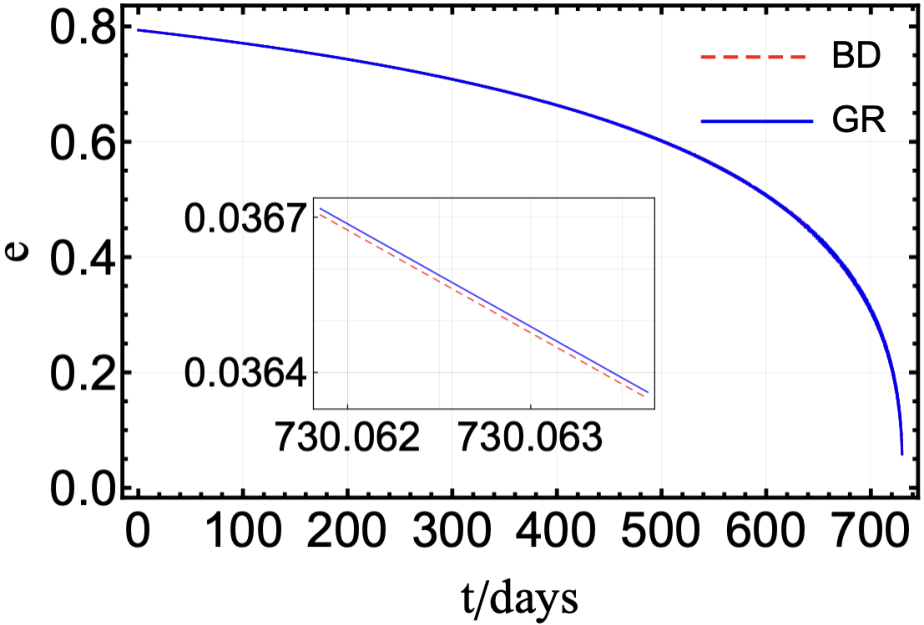
As an example, we consider a binary consisting of a NS and a BH. We take the mass of the NS as $m_{2}=1.3M_{\odot}$, the sensitivity as $s_{2}=0.2$ [66], and the mass ratio between the NS and the BH as $q=m_{2}/m_{1}=10^{-4}$. With these choices of the parameters, we get $s_{2}^{\prime}=s_{2}^{\prime\prime}=0$, and the PN parameters $\bar{\gamma}=\bar{\beta}_{1}=\bar{\beta}_{2}=\bar{\delta}_{1}=\bar{\chi}_{1}=\bar{\chi}_{2}=0$. The initial conditions are as follows: at the initial time $t_{0}=0$, the dimensionless semilatus rectum $p_{0}=80$, the eccentricity $e_{0}=0.8$ [113, 149], the orbital parameter at periapsis $\xi_{0}=10$, and the phase at periapsis $\phi_{0}=0$. The results for the orbital evolution are shown in figures 2 and 3. Figure 2 plots the orbital evolutions and figure 3 plots the evolution of the eccentricity $e$. It is shown that the difference of the evolution of the eccentricity between BD and GR is very small. We also considered the cases with $q=10^{-3}$ and $q=10^{-6}$.

From figure 2, we see that during the initial inspirals, the orbits in GR and BD theory are almost identical. The orbits in the BD theory with $\omega_{0}=(10^{4},10^{5},10^{6})$ start to deviate from those in GR after $t=(18,24,24)$ months of inspirals, respectively. The main difference in the orbital evolution can be manifested by the orbital phase accumulation. In figure 4, we show the evolutions of the orbital phase difference $\Delta\phi=\langle\phi_{\text{BD}}\rangle-\langle\phi_{\text{GR}}\rangle$ between GR and BD theory with different $\omega_{0}$ and $q$, here $\langle\phi\rangle$ means the phase average over one cycle. As expected, the phase difference increases as $\omega_{0}$ becomes smaller which is consistent with the results of the orbital evolution. After around one-year inspiral, the phase difference is 273.4 rad for $\omega_{0}=2000$ and $q=10^{-3}$; the phase difference is larger than 40 rad for $\omega_{0}=2000$ and $q=10^{-4}$; and the phase difference is 1.62 rad for $\omega_{0}=50000$ and $q=10^{-4}$. After around two-year inspiral, the phase difference is 81.93 rad for $\omega_{0}=10^{4}$ and $q=10^{-3}$; the phase difference is larger than 17.24 rad for $\omega_{0}=10^{4}$ and $q=10^{-4}$; the phase difference is 2.24 rad for $\omega_{0}=10^{5}$ and $q=10^{-4}$; and the phase difference is 0.94 rad for $\omega_{0}=10^{6}$ and $q=10^{-4}$. As the mass of the central BH increases, the accumulated phase difference decreases. Note that the difference of the number of cycles the NS inspiralled between GR and BD theory is $\Delta N=\Delta\phi/(2\pi)$. If we can observe the motion of the NS, then we can use $\Delta N$ to distinguish BD theory from GR. The accumulated phase difference will be manifested in the GW waveform and make it possible to constrain BD.

For GR, the waveform up to quadrupole radiation is

$$h^{ij}_{\text{GR}}=\frac{4\eta m}{D_{L}}\left(v^{i}v^{j}-\frac{m}{r}n^{i}n^{j}\right),$$

(3.1)

and for BD, the waveform up to quadrupole radiation is [61]

$$h^{ij}_{BD}=-\frac{2\zeta\mathcal{A}}{D_{L}}(\delta^{ij}-\Omega^{i}\Omega^{j})+\frac{4(1-2\zeta)\eta m}{D_{L}}(v^{i}v^{j}-\frac{m}{r}n^{i}n^{j}),$$

(3.2)

where $D_{L}$ is the luminosity distance between the source and the detector and the unit vector $\bm{\Omega}$ is the propagation direction of GWs. The other parameters are

$$\mathcal{A}=\mathcal{E}+\dot{\mathcal{E}}^{j}\Omega_{j}-\frac{1}{2}\ddot{I}^{jk}\Omega_{j}\Omega_{k},$$

(3.3)

$$\mathcal{E}=2(1+2\lambda)\frac{m_{1}m_{2}}{r}+\eta m\left[v^{2}+(1+4\lambda)\frac{m}{r}\right],$$

(3.4)

$$\mathcal{E}^{j}=-2(1+2\lambda)\eta m\mathcal{S}r^{j}-\eta\Delta m\left[v^{2}+(1+4\lambda)\frac{m}{2r}\right]r^{j},$$

(3.5)

$$\ddot{I}^{jk}=2\eta m\left(v^{i}v^{j}-\frac{m}{r}n^{i}n^{j}\right),$$

(3.6)

where $\Delta=(m_{1}-m_{2})/(m_{1}+m_{2})$ and $\mathcal{S}=(m_{1}-m_{2})/(2r)$. For GWs propagating along the $z$ direction with the unit vector $e_{Z}$ in the detector-adapted frame, the polarizations of GWs are expressed as

$$h_{+}=\frac{1}{2}h_{ij}(e^{i}_{X}e^{j}_{X}-e^{i}_{Y}e^{j}_{Y}),$$

(3.7)

$$h_{\times}=\frac{1}{2}h_{ij}(e^{i}_{X}e^{j}_{Y}+e^{j}_{X}e^{i}_{Y}),$$

(3.8)

$$h_{b}=\frac{1}{2}h_{ij}(e^{i}_{X}e^{j}_{X}+e^{i}_{Y}e^{j}_{Y}),$$

(3.9)

where the unit vectors $e_{X}$ and $e_{Y}$ are perpendicular to the unit vector $e_{Z}$ and they along with $e_{Z}$ form an orthonormal basis. In the absence of the BD scalar field, GR is recovered, $h_{+}$ and $h_{\times}$ are the plus and cross polarizations in the transverse-tracefree (TT) gauge. In particular, in the heliocentric coordinate system,

$$\begin{split}e_{X}&=[\cos\xi,\sin\xi,0],\\ e_{Y}&=[-\cos\iota\sin\xi,\cos\iota\cos\xi,\sin\iota],\end{split}$$

(3.10)

where the inclination angle $\iota$ measures the angle between the propagation direction of GWs and the normal vector of the orbital plane, the longitude of pericenter $\xi$ is the angle between the pericenter and the line of nodes as measured in the orbital plane.

References

- [1] LIGO Scientific and Virgo Collaborations collaboration, Observation of Gravitational Waves from a Binary Black Hole Merger, Phys. Rev. Lett. 116 (2016) 061102 [1602.03837].
- [2] LIGO Scientific and Virgo Collaborations collaboration, GW150914: The Advanced LIGO Detectors in the Era of First Discoveries, Phys. Rev. Lett. 116 (2016) 131103 [1602.03838].
- [3] LIGO Scientific Collaboration collaboration, Advanced LIGO: The next generation of gravitational wave detectors, Class. Quant. Grav. 27 (2010) 084006.
- [4] LIGO Scientific Collaboration collaboration, Advanced LIGO, Class. Quant. Grav. 32 (2015) 074001 [1411.4547].
- [5] VIRGO Collaboration collaboration, Advanced Virgo: a second-generation interferometric gravitational wave detector, Class. Quant. Grav. 32 (2015) 024001 [1408.3978].
- [6] LIGO Scientific and Virgo Collaborations collaboration, GWTC-1: A Gravitational-Wave Transient Catalog of Compact Binary Mergers Observed by LIGO and Virgo during the First and Second Observing Runs, Phys. Rev. X 9 (2019) 031040 [1811.12907].
- [7] LIGO Scientific and VIRGO Collaborations collaboration, GWTC-2: Compact Binary Coalescences Observed by LIGO and Virgo During the First Half of the Third Observing Run, Phys. Rev. X 11 (2021) 021053 [2010.14527].
- [8] LIGO Scientific and VIRGO Collaborations collaboration, GWTC-2.1: Deep Extended Catalog of Compact Binary Coalescences Observed by LIGO and Virgo During the First Half of the Third Observing Run, 2108.01045.
- [9] LIGO Scientific, VIRGO and KAGRA Collaborations collaboration, GWTC-3: Compact Binary Coalescences Observed by LIGO and Virgo During the Second Part of the Third Observing Run, 2111.03606.
- [10] D. M. Eardley, D. L. Lee, A. P. Lightman, R. V. Wagoner and C. M. Will, Gravitational-wave observations as a tool for testing relativistic gravity, Phys. Rev. Lett. 30 (1973) 884.
- [11] D. M. Eardley, D. L. Lee and A. P. Lightman, Gravitational-wave observations as a tool for testing relativistic gravity, Phys. Rev. D 8 (1973) 3308.
- [12] R. V. Wagoner, Scalar tensor theory and gravitational waves, Phys. Rev. D 1 (1970) 3209.
- [13] D. Liang, Y. Gong, S. Hou and Y. Liu, Polarizations of gravitational waves in gravity, Phys. Rev. D 95 (2017) 104034 [1701.05998].
- [14] S. Hou, Y. Gong and Y. Liu, Polarizations of Gravitational Waves in Horndeski Theory, Eur. Phys. J. C 78 (2018) 378 [1704.01899].
- [15] Y. Gong, S. Hou, E. Papantonopoulos and D. Tzortzis, Gravitational waves and the polarizations in Hořava gravity after GW170817, Phys. Rev. D 98 (2018) 104017 [1808.00632].
- [16] Y. Gong, S. Hou, D. Liang and E. Papantonopoulos, Gravitational waves in Einstein-æther and generalized TeVeS theory after GW170817, Phys. Rev. D 97 (2018) 084040 [1801.03382].
- [17] LIGO Scientific and Virgo Collaborations collaboration, Tests of general relativity with GW150914, Phys. Rev. Lett. 116 (2016) 221101 [1602.03841].
- [18] LIGO Scientific and Virgo Collaborations collaboration, Tests of General Relativity with GW170817, Phys. Rev. Lett. 123 (2019) 011102 [1811.00364].
- [19] LIGO Scientific and Virgo Collaborations collaboration, Tests of General Relativity with the Binary Black Hole Signals from the LIGO-Virgo Catalog GWTC-1, Phys. Rev. D 100 (2019) 104036 [1903.04467].
- [20] LIGO Scientific and Virgo Collaborations collaboration, Tests of general relativity with binary black holes from the second LIGO-Virgo gravitational-wave transient catalog, Phys. Rev. D 103 (2021) 122002 [2010.14529].
- [21] LIGO Scientific, Virgo, Fermi-GBM and INTEGRAL Collaborations collaboration, Gravitational Waves and Gamma-rays from a Binary Neutron Star Merger: GW170817 and GRB 170817A, Astrophys. J. Lett. 848 (2017) L13 [1710.05834].
- [22] S. Mirshekari, N. Yunes and C. M. Will, Constraining Generic Lorentz Violation and the Speed of the Graviton with Gravitational Waves, Phys. Rev. D 85 (2012) 024041 [1110.2720].
- [23] J. Beltran Jimenez, F. Piazza and H. Velten, Evading the Vainshtein Mechanism with Anomalous Gravitational Wave Speed: Constraints on Modified Gravity from Binary Pulsars, Phys. Rev. Lett. 116 (2016) 061101 [1507.05047].
- [24] P. M. Chesler and A. Loeb, Constraining Relativistic Generalizations of Modified Newtonian Dynamics with Gravitational Waves, Phys. Rev. Lett. 119 (2017) 031102 [1704.05116].
- [25] T. Baker, E. Bellini, P. G. Ferreira, M. Lagos, J. Noller and I. Sawicki, Strong constraints on cosmological gravity from GW170817 and GRB 170817A, Phys. Rev. Lett. 119 (2017) 251301 [1710.06394].
- [26] P. Creminelli and F. Vernizzi, Dark Energy after GW170817 and GRB170817A, Phys. Rev. Lett. 119 (2017) 251302 [1710.05877].
- [27] J. Sakstein and B. Jain, Implications of the Neutron Star Merger GW170817 for Cosmological Scalar-Tensor Theories, Phys. Rev. Lett. 119 (2017) 251303 [1710.05893].
- [28] J. M. Ezquiaga and M. Zumalacárregui, Dark Energy After GW170817: Dead Ends and the Road Ahead, Phys. Rev. Lett. 119 (2017) 251304 [1710.05901].
- [29] M. A. Green, J. W. Moffat and V. T. Toth, Modified Gravity (MOG), the speed of gravitational radiation and the event GW170817/GRB170817A, Phys. Lett. B 780 (2018) 300 [1710.11177].
- [30] A. Nishizawa, Generalized framework for testing gravity with gravitational-wave propagation. I. Formulation, Phys. Rev. D 97 (2018) 104037 [1710.04825].
- [31] S. Arai and A. Nishizawa, Generalized framework for testing gravity with gravitational-wave propagation. II. Constraints on Horndeski theory, Phys. Rev. D 97 (2018) 104038 [1711.03776].
- [32] Y. Gong, E. Papantonopoulos and Z. Yi, Constraints on scalar–tensor theory of gravity by the recent observational results on gravitational waves, Eur. Phys. J. C 78 (2018) 738 [1711.04102].
- [33] R. A. Battye, F. Pace and D. Trinh, Gravitational wave constraints on dark sector models, Phys. Rev. D 98 (2018) 023504 [1802.09447].
- [34] A. Casalino, M. Rinaldi, L. Sebastiani and S. Vagnozzi, Mimicking dark matter and dark energy in a mimetic model compatible with GW170817, Phys. Dark Univ. 22 (2018) 108 [1803.02620].
- [35] A. Casalino, M. Rinaldi, L. Sebastiani and S. Vagnozzi, Alive and well: mimetic gravity and a higher-order extension in light of GW170817, Class. Quant. Grav. 36 (2019) 017001 [1811.06830].
- [36] L. Visinelli, N. Bolis and S. Vagnozzi, Brane-world extra dimensions in light of GW170817, Phys. Rev. D 97 (2018) 064039 [1711.06628].
- [37] C. Brans and R. H. Dicke, Mach’s principle and a relativistic theory of gravitation, Phys. Rev. 124 (1961) 925.
- [38] R. H. Dicke, Mach’s principle and invariance under transformation of units, Phys. Rev. 125 (1962) 2163.
- [39] A. Avilez and C. Skordis, Cosmological constraints on Brans-Dicke theory, Phys. Rev. Lett. 113 (2014) 011101 [1303.4330].
- [40] D. Alonso, E. Bellini, P. G. Ferreira and M. Zumalacárregui, Observational future of cosmological scalar-tensor theories, Phys. Rev. D 95 (2017) 063502 [1610.09290].
- [41] H. Amirhashchi and A. K. Yadav, Constraining an exact Brans-Dicke gravity theory with recent observations, Phys. Dark Univ. 30 (2020) 100711 [1908.04735].
- [42] B. Bertotti, L. Iess and P. Tortora, A test of general relativity using radio links with the Cassini spacecraft, Nature 425 (2003) 374.
- [43] C. M. Will, The Confrontation between General Relativity and Experiment, Living Rev. Rel. 17 (2014) 4 [1403.7377].
- [44] D. M. Eardley, Observable effects of a scalar gravitational field in a binary pulsar, Astrophys. J. 196 (1975) L59.
- [45] C. M. Will, Gravitational Radiation from Binary Systems in Alternative Metric Theories of Gravity: Dipole Radiation and the Binary Pulsar, Astrophys. J. 214 (1977) 826.
- [46] C. M. Will and H. W. Zaglauer, Gravitational Radiation, Close Binary Systems, and the Brans-dicke Theory of Gravity, Astrophys. J. 346 (1989) 366.
- [47] T. Damour and G. Esposito-Farese, Tensor multiscalar theories of gravitation, Class. Quant. Grav. 9 (1992) 2093.
- [48] T. Damour and G. Esposito-Farese, Gravitational wave versus binary - pulsar tests of strong field gravity, Phys. Rev. D 58 (1998) 042001 [gr-qc/9803031].
- [49] J. Alsing, E. Berti, C. M. Will and H. Zaglauer, Gravitational radiation from compact binary systems in the massive Brans-Dicke theory of gravity, Phys. Rev. D 85 (2012) 064041 [1112.4903].
- [50] J. Antoniadis et al., A Massive Pulsar in a Compact Relativistic Binary, Science 340 (2013) 6131 [1304.6875].
- [51] X. Zhang, R. Niu and W. Zhao, Constraining the scalar-tensor gravity theories with and without screening mechanisms by combined observations, Phys. Rev. D 100 (2019) 024038 [1906.10791].
- [52] B. C. Seymour and K. Yagi, Probing Massive Scalar Fields from a Pulsar in a Stellar Triple System, Class. Quant. Grav. 37 (2020) 145008 [1908.03353].
- [53] P. C. C. Freire, N. Wex, G. Esposito-Farese, J. P. W. Verbiest, M. Bailes, B. A. Jacoby et al., The relativistic pulsar-white dwarf binary PSR J1738+0333 II. The most stringent test of scalar-tensor gravity, Mon. Not. Roy. Astron. Soc. 423 (2012) 3328 [1205.1450].
- [54] S. Mirshekari and C. M. Will, Compact binary systems in scalar-tensor gravity: Equations of motion to 2.5 post-Newtonian order, Phys. Rev. D 87 (2013) 084070 [1301.4680].
- [55] R. N. Lang, Compact binary systems in scalar-tensor gravity. II. Tensor gravitational waves to second post-Newtonian order, Phys. Rev. D 89 (2014) 084014 [1310.3320].
- [56] R. N. Lang, Compact binary systems in scalar-tensor gravity. III. Scalar waves and energy flux, Phys. Rev. D 91 (2015) 084027 [1411.3073].
- [57] N. Sennett, S. Marsat and A. Buonanno, Gravitational waveforms in scalar-tensor gravity at 2PN relative order, Phys. Rev. D 94 (2016) 084003 [1607.01420].
- [58] L. Bernard, Dynamics of compact binary systems in scalar-tensor theories: Equations of motion to the third post-Newtonian order, Phys. Rev. D 98 (2018) 044004 [1802.10201].
- [59] L. Bernard, Dynamics of compact binary systems in scalar-tensor theories: II. Center-of-mass and conserved quantities to 3PN order, Phys. Rev. D 99 (2019) 044047 [1812.04169].
- [60] L. Bernard, Dipolar tidal effects in scalar-tensor theories, Phys. Rev. D 101 (2020) 021501 [1906.10735].
- [61] C. M. Will, Testing scalar - tensor gravity with gravitational wave observations of inspiraling compact binaries, Phys. Rev. D 50 (1994) 6058 [gr-qc/9406022].
- [62] M. Shibata, K.-i. Nakao and T. Nakamura, Scalar type gravitational wave emission from gravitational collapse in Brans-Dicke theory: Detectability by a laser interferometer, Phys. Rev. D 50 (1994) 7304.
- [63] M. Saijo, H.-a. Shinkai and K.-i. Maeda, Gravitational waves in Brans-Dicke theory : Analysis by test particles around a Kerr black hole, Phys. Rev. D 56 (1997) 785 [gr-qc/9701001].
- [64] C. M. Will, Bounding the mass of the graviton using gravitational wave observations of inspiralling compact binaries, Phys. Rev. D 57 (1998) 2061 [gr-qc/9709011].
- [65] M. Brunetti, E. Coccia, V. Fafone and F. Fucito, Gravitational wave radiation from compact binary systems in the Jordan-Brans-Dicke theory, Phys. Rev. D 59 (1999) 044027 [gr-qc/9805056].
- [66] P. D. Scharre and C. M. Will, Testing scalar tensor gravity using space gravitational wave interferometers, Phys. Rev. D 65 (2002) 042002 [gr-qc/0109044].
- [67] C. M. Will and N. Yunes, Testing alternative theories of gravity using LISA, Class. Quant. Grav. 21 (2004) 4367 [gr-qc/0403100].
- [68] E. Berti, A. Buonanno and C. M. Will, Estimating spinning binary parameters and testing alternative theories of gravity with LISA, Phys. Rev. D 71 (2005) 084025 [gr-qc/0411129].
- [69] K. Yagi and T. Tanaka, Constraining alternative theories of gravity by gravitational waves from precessing eccentric compact binaries with LISA, Phys. Rev. D 81 (2010) 064008 [0906.4269].
- [70] N. Yunes, P. Pani and V. Cardoso, Gravitational Waves from Quasicircular Extreme Mass-Ratio Inspirals as Probes of Scalar-Tensor Theories, Phys. Rev. D 85 (2012) 102003 [1112.3351].
- [71] K. G. Arun, Generic bounds on dipolar gravitational radiation from inspiralling compact binaries, Class. Quant. Grav. 29 (2012) 075011 [1202.5911].
- [72] E. Barausse, N. Yunes and K. Chamberlain, Theory-Agnostic Constraints on Black-Hole Dipole Radiation with Multiband Gravitational-Wave Astrophysics, Phys. Rev. Lett. 116 (2016) 241104 [1603.04075].
- [73] F.-L. Julié, Reducing the two-body problem in scalar-tensor theories to the motion of a test particle : a scalar-tensor effective-one-body approach, Phys. Rev. D 97 (2018) 024047 [1709.09742].
- [74] G. Gnocchi, A. Maselli, T. Abdelsalhin, N. Giacobbo and M. Mapelli, Bounding alternative theories of gravity with multiband GW observations, Phys. Rev. D 100 (2019) 064024 [1905.13460].
- [75] Z. Carson, B. C. Seymour and K. Yagi, Future prospects for probing scalar–tensor theories with gravitational waves from mixed binaries, Class. Quant. Grav. 37 (2020) 065008 [1907.03897].
- [76] S. Ma and N. Yunes, Improved Constraints on Modified Gravity with Eccentric Gravitational Waves, Phys. Rev. D 100 (2019) 124032 [1908.07089].
- [77] B. Moore and N. Yunes, Constraining Gravity with Eccentric Gravitational Waves: Projected Upper Bounds and Model Selection, Class. Quant. Grav. 37 (2020) 165006 [2002.05775].
- [78] B. C. Seymour and K. Yagi, Probing massive scalar and vector fields with binary pulsars, Phys. Rev. D 102 (2020) 104003 [2007.14881].
- [79] R. Niu, X. Zhang, B. Wang and W. Zhao, Constraining Scalar-tensor Theories Using Neutron Star–Black Hole Gravitational Wave Events, Astrophys. J. 921 (2021) 149 [2105.13644].
- [80] K. Danzmann, LISA: An ESA cornerstone mission for a gravitational wave observatory, Class. Quant. Grav. 14 (1997) 1399.
- [81] LISA Collaboration collaboration, Laser Interferometer Space Antenna, 1702.00786.
- [82] TianQin Collaboration collaboration, TianQin: a space-borne gravitational wave detector, Class. Quant. Grav. 33 (2016) 035010 [1512.02076].
- [83] W.-R. Hu and Y.-L. Wu, The Taiji Program in Space for gravitational wave physics and the nature of gravity, Natl. Sci. Rev. 4 (2017) 685.
- [84] Y. Gong, J. Luo and B. Wang, Concepts and status of Chinese space gravitational wave detection projects, Nature Astron. 5 (2021) 881 [2109.07442].
- [85] G. Fragione, I. Ginsburg and B. Kocsis, Gravitational Waves and Intermediate-mass Black Hole Retention in Globular Clusters, Astrophys. J. 856 (2018) 92 [1711.00483].
- [86] M. C. Miller and D. P. Hamilton, Production of intermediate-mass black holes in globular clusters, Mon. Not. Roy. Astron. Soc. 330 (2002) 232 [astro-ph/0106188].
- [87] M. C. Miller, Probing general relativity with mergers of supermassive and intermediate-mass black holes, Astrophys. J. 618 (2004) 426 [astro-ph/0409331].
- [88] L. Barack and A. Pound, Self-force and radiation reaction in general relativity, Rept. Prog. Phys. 82 (2019) 016904 [1805.10385].
- [89] C. Cutler and E. E. Flanagan, Gravitational waves from merging compact binaries: How accurately can one extract the binary’s parameters from the inspiral wave form?, Phys. Rev. D 49 (1994) 2658 [gr-qc/9402014].
- [90] Y. Kozai, Secular perturbations of asteroids with high inclination and eccentricity, Astron. J. 67 (1962) 591.
- [91] D. C. Heggie, Binary evolution in stellar dynamics, Mon. Not. Roy. Astron. Soc. 173 (1975) 729.
- [92] L. Wen, On the eccentricity distribution of coalescing black hole binaries driven by the Kozai mechanism in globular clusters, Astrophys. J. 598 (2003) 419 [astro-ph/0211492].
- [93] M. C. Miller and D. P. Hamilton, Four-body effects in globular cluster black hole coalescence, Astrophys. J. 576 (2002) 894 [astro-ph/0202298].
- [94] J. Samsing, A. Askar and M. Giersz, MOCCA-SURVEY Database. I. Eccentric Black Hole Mergers during Binary–Single Interactions in Globular Clusters, Astrophys. J. 855 (2018) 124 [1712.06186].
- [95] C. L. Rodriguez, P. Amaro-Seoane, S. Chatterjee and F. A. Rasio, Post-Newtonian Dynamics in Dense Star Clusters: Highly-Eccentric, Highly-Spinning, and Repeated Binary Black Hole Mergers, Phys. Rev. Lett. 120 (2018) 151101 [1712.04937].
- [96] D. J. D’Orazio and J. Samsing, Black Hole Mergers From Globular Clusters Observable by LISA II: Resolved Eccentric Sources and the Gravitational Wave Background, Mon. Not. Roy. Astron. Soc. 481 (2018) 4775 [1805.06194].
- [97] B.-M. Hoang, S. Naoz, B. Kocsis, W. Farr and J. McIver, Detecting Supermassive Black Hole–induced Binary Eccentricity Oscillations with LISA, Astrophys. J. Lett. 875 (2019) L31 [1903.00134].
- [98] A. H. Mroue, H. P. Pfeiffer, L. E. Kidder and S. A. Teukolsky, Measuring orbital eccentricity and periastron advance in quasi-circular black hole simulations, Phys. Rev. D 82 (2010) 124016 [1004.4697].
- [99] A. Nishizawa, E. Berti, A. Klein and A. Sesana, eLISA eccentricity measurements as tracers of binary black hole formation, Phys. Rev. D 94 (2016) 064020 [1605.01341].
- [100] A. Nishizawa, A. Sesana, E. Berti and A. Klein, Constraining stellar binary black hole formation scenarios with eLISA eccentricity measurements, Mon. Not. Roy. Astron. Soc. 465 (2017) 4375 [1606.09295].
- [101] K. Breivik, C. L. Rodriguez, S. L. Larson, V. Kalogera and F. A. Rasio, Distinguishing Between Formation Channels for Binary Black Holes with LISA, Astrophys. J. Lett. 830 (2016) L18 [1606.09558].
- [102] L. Gondán, B. Kocsis, P. Raffai and Z. Frei, Accuracy of Estimating Highly Eccentric Binary Black Hole Parameters with Gravitational-Wave Detections, Astrophys. J. 855 (2018) 34 [1705.10781].
- [103] L. Gondán and B. Kocsis, Measurement Accuracy of Inspiraling Eccentric Neutron Star and Black Hole Binaries Using Gravitational Waves, Astrophys. J. 871 (2019) 178 [1809.00672].
- [104] B. Moore and N. Yunes, Data Analysis Implications of Moderately Eccentric Gravitational Waves, Class. Quant. Grav. 37 (2020) 225015 [1910.01680].
- [105] S. Wu, Z. Cao and Z.-H. Zhu, Measuring the eccentricity of binary black holes in GWTC-1 by using the inspiral-only waveform, Mon. Not. Roy. Astron. Soc. 495 (2020) 466 [2002.05528].
- [106] A. K. Lenon, A. H. Nitz and D. A. Brown, Measuring the eccentricity of GW170817 and GW190425, Mon. Not. Roy. Astron. Soc. 497 (2020) 1966 [2005.14146].
- [107] M. Favata, C. Kim, K. G. Arun, J. Kim and H. W. Lee, Constraining the orbital eccentricity of inspiralling compact binary systems with Advanced LIGO, Phys. Rev. D 105 (2022) 023003 [2108.05861].
- [108] W. Junker and G. Schäfer, Binary systems: higher order gravitational radiation damping and wave emission, Mon. Not. Roy. Astron. Soc. 254 (1992) 146.
- [109] A. Krolak, K. D. Kokkotas and G. Schaefer, On estimation of the postNewtonian parameters in the gravitational wave emission of a coalescing binary, Phys. Rev. D 52 (1995) 2089 [gr-qc/9503013].
- [110] L. Blanchet, T. Damour, B. R. Iyer, C. M. Will and A. G. Wiseman, Gravitational radiation damping of compact binary systems to second postNewtonian order, Phys. Rev. Lett. 74 (1995) 3515 [gr-qc/9501027].
- [111] M. Vallisneri, Use and abuse of the Fisher information matrix in the assessment of gravitational-wave parameter-estimation prospects, Phys. Rev. D 77 (2008) 042001 [gr-qc/0703086].
- [112] K. J. Shuman and N. J. Cornish, Massive black hole binaries and where to find them with dual detector networks, Phys. Rev. D 105 (2022) 064055 [2105.02943].
- [113] L. Barack and C. Cutler, LISA capture sources: Approximate waveforms, signal-to-noise ratios, and parameter estimation accuracy, Phys. Rev. D 69 (2004) 082005 [gr-qc/0310125].
- [114] S. A. Teukolsky, Perturbations of a rotating black hole. 1. Fundamental equations for gravitational electromagnetic and neutrino field perturbations, Astrophys. J. 185 (1973) 635.
- [115] S. Babak, H. Fang, J. R. Gair, K. Glampedakis and S. A. Hughes, ’Kludge’ gravitational waveforms for a test-body orbiting a Kerr black hole, Phys. Rev. D 75 (2007) 024005 [gr-qc/0607007].
- [116] A. J. K. Chua and J. R. Gair, Improved analytic extreme-mass-ratio inspiral model for scoping out eLISA data analysis, Class. Quant. Grav. 32 (2015) 232002 [1510.06245].
- [117] A. J. K. Chua, C. J. Moore and J. R. Gair, Augmented kludge waveforms for detecting extreme-mass-ratio inspirals, Phys. Rev. D 96 (2017) 044005 [1705.04259].
- [118] L. Barack, Gravitational self force in extreme mass-ratio inspirals, Class. Quant. Grav. 26 (2009) 213001 [0908.1664].
- [119] E. Poisson, A. Pound and I. Vega, The Motion of point particles in curved spacetime, Living Rev. Rel. 14 (2011) 7 [1102.0529].
- [120] Y. Mino, M. Sasaki and T. Tanaka, Gravitational radiation reaction to a particle motion, Phys. Rev. D 55 (1997) 3457 [gr-qc/9606018].
- [121] T. C. Quinn and R. M. Wald, An Axiomatic approach to electromagnetic and gravitational radiation reaction of particles in curved space-time, Phys. Rev. D 56 (1997) 3381 [gr-qc/9610053].
- [122] L. Barack and A. Ori, Mode sum regularization approach for the selfforce in black hole space-time, Phys. Rev. D 61 (2000) 061502 [gr-qc/9912010].
- [123] C. O. Lousto, Pragmatic approach to gravitational radiation reaction in binary black holes, Phys. Rev. Lett. 84 (2000) 5251 [gr-qc/9912017].
- [124] L. M. Burko, Selfforce on particle in orbit around a black hole, Phys. Rev. Lett. 84 (2000) 4529 [gr-qc/0003074].
- [125] S. L. Detweiler, Radiation reaction and the selfforce for a point mass in general relativity, Phys. Rev. Lett. 86 (2001) 1931 [gr-qc/0011039].
- [126] M. J. Pfenning and E. Poisson, Scalar, electromagnetic, and gravitational selfforces in weakly curved space-times, Phys. Rev. D 65 (2002) 084001 [gr-qc/0012057].
- [127] L. Barack, Y. Mino, H. Nakano, A. Ori and M. Sasaki, Calculating the gravitational selfforce in Schwarzschild space-time, Phys. Rev. Lett. 88 (2002) 091101 [gr-qc/0111001].
- [128] L. Barack, Gravitational selfforce by mode sum regularization, Phys. Rev. D 64 (2001) 084021 [gr-qc/0105040].
- [129] L. Barack and C. O. Lousto, Computing the gravitational selfforce on a compact object plunging into a Schwarzschild black hole, Phys. Rev. D 66 (2002) 061502 [gr-qc/0205043].
- [130] T. S. Keidl, J. L. Friedman and A. G. Wiseman, On finding fields and self-force in a gauge appropriate to separable wave equations, Phys. Rev. D 75 (2007) 124009 [gr-qc/0611072].
- [131] L. Barack and D. A. Golbourn, Scalar-field perturbations from a particle orbiting a black hole using numerical evolution in 2+1 dimensions, Phys. Rev. D 76 (2007) 044020 [0705.3620].
- [132] A. C. Ottewill and B. Wardell, Quasilocal contribution to the scalar self-force: Geodesic motion, Phys. Rev. D 77 (2008) 104002 [0711.2469].
- [133] S. L. Detweiler, A Consequence of the gravitational self-force for circular orbits of the Schwarzschild geometry, Phys. Rev. D 77 (2008) 124026 [0804.3529].
- [134] L. Barack and N. Sago, Gravitational self-force correction to the innermost stable circular orbit of a Schwarzschild black hole, Phys. Rev. Lett. 102 (2009) 191101 [0902.0573].
- [135] L. Barack and N. Sago, Gravitational self-force on a particle in eccentric orbit around a Schwarzschild black hole, Phys. Rev. D 81 (2010) 084021 [1002.2386].
- [136] A. Le Tiec, A. H. Mroue, L. Barack, A. Buonanno, H. P. Pfeiffer, N. Sago et al., Periastron Advance in Black Hole Binaries, Phys. Rev. Lett. 107 (2011) 141101 [1106.3278].
- [137] P. Diener, I. Vega, B. Wardell and S. Detweiler, Self-consistent orbital evolution of a particle around a Schwarzschild black hole, Phys. Rev. Lett. 108 (2012) 191102 [1112.4821].
- [138] A. Pound, Second-order gravitational self-force, Phys. Rev. Lett. 109 (2012) 051101 [1201.5089].
- [139] S. Isoyama, L. Barack, S. R. Dolan, A. Le Tiec, H. Nakano, A. G. Shah et al., Gravitational Self-Force Correction to the Innermost Stable Circular Equatorial Orbit of a Kerr Black Hole, Phys. Rev. Lett. 113 (2014) 161101 [1404.6133].
- [140] P. Zimmerman, Gravitational self-force in scalar-tensor gravity, Phys. Rev. D 92 (2015) 064051 [1507.04076].
- [141] M. van de Meent, Self-force corrections to the periapsis advance around a spinning black hole, Phys. Rev. Lett. 118 (2017) 011101 [1610.03497].
- [142] A. Pound, B. Wardell, N. Warburton and J. Miller, Second-Order Self-Force Calculation of Gravitational Binding Energy in Compact Binaries, Phys. Rev. Lett. 124 (2020) 021101 [1908.07419].
- [143] A. Antonelli, C. Kavanagh, M. Khalil, J. Steinhoff and J. Vines, Gravitational spin-orbit coupling through third-subleading post-Newtonian order: from first-order self-force to arbitrary mass ratios, Phys. Rev. Lett. 125 (2020) 011103 [2003.11391].
- [144] A. Nagar and S. Albanesi, Towards a gravitational self force-informed effective-one-body waveform model for nonprecessing, eccentric, large-mass-ratio inspirals, 2207.14002.
- [145] A. Albertini, A. Nagar, A. Pound, N. Warburton, B. Wardell, L. Durkan et al., Comparing second-order gravitational self-force, numerical relativity and effective one body waveforms from inspiralling, quasi-circular and nonspinning black hole binaries, 2208.01049.
- [146] M. Van De Meent and N. Warburton, Fast Self-forced Inspirals, Class. Quant. Grav. 35 (2018) 144003 [1802.05281].
- [147] A. Pound and E. Poisson, Osculating orbits in Schwarzschild spacetime, with an application to extreme mass-ratio inspirals, Phys. Rev. D 77 (2008) 044013 [0708.3033].
- [148] N. Warburton, S. Akcay, L. Barack, J. R. Gair and N. Sago, Evolution of inspiral orbits around a Schwarzschild black hole, Phys. Rev. D 85 (2012) 061501(R) [1111.6908].
- [149] T. Osburn, N. Warburton and C. R. Evans, Highly eccentric inspirals into a black hole, Phys. Rev. D 93 (2016) 064024 [1511.01498].
- [150] C. Cutler, Angular resolution of the LISA gravitational wave detector, Phys. Rev. D 57 (1998) 7089 [gr-qc/9703068].
- [151] R. Schilling, Angular and frequency response of LISA, Class. Quant. Grav. 14 (1997) 1513.
- [152] S. L. Larson, W. A. Hiscock and R. W. Hellings, Sensitivity curves for spaceborne gravitational wave interferometers, Phys. Rev. D 62 (2000) 062001 [gr-qc/9909080].
- [153] C. Zhang, Y. Gong, B. Wang and C. Zhang, Accuracy of parameter estimations with a spaceborne gravitational wave observatory, Phys. Rev. D 103 (2021) 104066 [2012.01043].
- [154] T. Robson, N. J. Cornish and C. Liu, The construction and use of LISA sensitivity curves, Class. Quant. Grav. 36 (2019) 105011 [1803.01944].
- [155] B. Kocsis, N. Yunes and A. Loeb, Observable Signatures of EMRI Black Hole Binaries Embedded in Thin Accretion Disks, Phys. Rev. D 84 (2011) 024032 [1104.2322].
- [156] T. A. Apostolatos, Search templates for gravitational waves from precessing, inspiraling binaries, Phys. Rev. D 52 (1995) 605.
- [157] B. Allen, W. G. Anderson, P. R. Brady, D. A. Brown and J. D. E. Creighton, FINDCHIRP: An Algorithm for detection of gravitational waves from inspiraling compact binaries, Phys. Rev. D 85 (2012) 122006 [gr-qc/0509116].
- [158] LIGO Scientific and Virgo Collaborations collaboration, Effects of waveform model systematics on the interpretation of GW150914, Class. Quant. Grav. 34 (2017) 104002 [1611.07531].
- [159] S. Datta, R. Brito, S. Bose, P. Pani and S. A. Hughes, Tidal heating as a discriminator for horizons in extreme mass ratio inspirals, Phys. Rev. D 101 (2020) 044004 [1910.07841].
- [160] G. Bozzola and V. Paschalidis, General Relativistic Simulations of the Quasicircular Inspiral and Merger of Charged Black Holes: GW150914 and Fundamental Physics Implications, Phys. Rev. Lett. 126 (2021) 041103 [2006.15764].
- [161] E. E. Flanagan and S. A. Hughes, Measuring gravitational waves from binary black hole coalescences: 2. The Waves’ information and its extraction, with and without templates, Phys. Rev. D 57 (1998) 4566 [gr-qc/9710129].
- [162] L. Lindblom, B. J. Owen and D. A. Brown, Model Waveform Accuracy Standards for Gravitational Wave Data Analysis, Phys. Rev. D 78 (2008) 124020 [0809.3844].
- [163] S. T. McWilliams, B. J. Kelly and J. G. Baker, Observing mergers of non-spinning black-hole binaries, Phys. Rev. D 82 (2010) 024014 [1004.0961].
- [164] Chatziioannou, Katerina and Klein, Antoine and Yunes, Nicolás and Cornish, Neil, Constructing Gravitational Waves from Generic Spin-Precessing Compact Binary Inspirals, Phys. Rev. D 95 (2017) 104004 [1703.03967].