T-LoHo: A Bayesian Regularization Model for Structured Sparsity and Smoothness on Graphs

First we review the horseshoe prior (Carvalho et al., 2010), which provides a sparse estimate of $\bm{\beta}$ by shrinking small effects towards zero while maintaining robustness to large signals:

where $\mathcal{N}_{p}(\bm{m},\bm{V})$ denotes a $p$-dimensional multivariate normal distribution with mean $\bm{m}$ and covariance $\bm{V}$, and $C^{+}(0,\gamma)$ denotes a half-Cauchy distribution with density $p(\lambda)=2/[\pi\gamma(1+\lambda^{2}/\gamma^{2})]$ for $\lambda>0$. Here $\tau$ is a global shrinkage parameter with hyperparameter $\tau_{0}$ to enforce global shrinkage towards zero, $\{\lambda_{j}\}$ are local shrinkage parameters with heavy tails which allow some of the $\beta_{j}$’s to escape the shrinkage, and $\sigma^{2}$ is a scaling factor which is often assumed to be the noise variance.

Given a graph partition $\Pi$ of $G$, we seek a new joint prior distribution of $\bm{\beta}\in\mathbb{R}^{p}$ to impose sparse homogeneity assumption while incorporating the clustering structure of $\Pi$ . For example when $p=5$ and $\Pi=\{\{1\},\{2,4\},\{3,5\}\}$ as shown in fig. 1(a), we seek a distribution which lies on a 3-dimensional subspace $\{\bm{\beta}\in\mathbb{R}^{5}:\beta_{2}=\beta_{4},\beta_{3}=\beta_{5}\}$. In general, given a graph partition $\Pi$ with size $K$, we can construct a $K\times p$ matrix $\Phi$ from $\Pi$:

This $K\times p$ matrix $\Phi$ represents a projection from a $p$-dimensional space to a reduced $K$-dimensional space. Note that rows of $\Phi$ are mutually orthonormal so that $\Phi\Phi^{\top}=\mathbf{I}_{K}$. Using $\Phi$ obtained from $\Pi$, we introduce the low-rank horseshoe (LoHo) prior to impose sparse homogeneity assumption on $\bm{\beta}$:

See fig. 1(a) for an example of $\Phi$ and a covariance matrix $\Phi^{\top}\Lambda\Phi$. Note LoHo introduces a covariance matrix capturing clustering dependence among $\bm{\beta}$ and its marginal local shrinkage for simultaneous sparsity and fusion, a key distinction from most existing methods (Carvalho et al., 2010; Kyung et al., 2010; Shimamura et al., 2019) that assume independence or only dependence among $\bm{\beta}$ but not local shrinkage parameters. Since $K$ is assumed to be small relative to $p$, the covariance matrix $\Phi^{\top}\Lambda\Phi$ has low rank (i.e., $\operatorname{rank}(\Phi^{\top}\Lambda\Phi)=K<\!\!<p$), and thus LoHo does not have a density with respect to Lebesgue measure on $\mathbb{R}^{p}$. Instead, its distribution lies on the row space of $\Phi$ with $\operatorname{dim}(\operatorname{rowsp}(\Phi))=K$, and we can consider the transformation $\tilde{\bm{\beta}}=\Phi\bm{\beta}$ so that $\tilde{\bm{\beta}}$ has a $\mathcal{N}_{K}(\bm{0},\sigma^{2}\tau^{2}\Lambda)$ density with respect to Lebesgue measure on $\operatorname{rowsp}(\Phi)$. Observe that $\Phi^{\top}$ is the Moore–Penrose pseudoinverse of $\Phi$, which implies $\Phi^{\top}\Phi$ is a projection onto $\operatorname{rowsp}(\Phi)$ so that we can recover $\bm{\beta}=\Phi^{\top}\tilde{\bm{\beta}}$.

By assigning a half-Cauchy prior, global shrinkage parameter $\tau$ creates a strong pull towards zero while clusterwise local shrinkage parameters $\{\lambda_{k}\}_{k=1}^{K}$ allow some of the clusterwise $\tilde{\beta}_{k}$’s to escape the shrinkage. Assuming $\Phi$ having orthonormal rows is important in the sense that the effect of local shrinkage parameters $\{\lambda_{k}\}_{k=1}^{K}$ remains same across the clusters with varying size. Thus using the projection onto the low-dimensional subspace, LoHo gives more parsimonious estimate of $\bm{\beta}$ by forming clusters of zero and non-zero parameters.

LoHo can be naturally incorporated into a linear model. With response vector $\bm{y}\in\mathbb{R}^{n}$ and column-standardized design matrix $\mathbf{X}\in\mathbb{R}^{n\times p}$ so that each column has unit $\ell_{2}$ norm, we can write

Under this formulation, LoHo has a close connection with Bayesian compressed regression (Guhaniyogi and Dunson, 2015). It randomly projects predictors $\mathbf{X}_{i}\mapsto\Phi\mathbf{X}_{i}$ with a certain family of matrix $\Phi$ and performs model averaging, at the cost of losing interpretability of $\bm{\beta}$. But LoHo directly introduces a prior on $\bm{\beta}$ using the projection matrix $\Phi$ defined as (1) so that it induces clustered coefficient while maintaining interpretability of $\bm{\beta}$. Also, functional horseshoe (Shin et al., 2020) shrinks $\mathbf{X}\bm{\beta}$ towards the subspace of $\operatorname{colsp}(\mathbf{X})$ while LoHo shrinks $\bm{\beta}$ towards $\bm{0}$ along the $\operatorname{rowsp}(\Phi)$.

We remark that, although it appears $(\tau,\Lambda)$ and $\Phi$ handle sparsity and homogeneity separately, shrinkage component in LoHo also affects clustering by facilitating cluster fusion when signal is low and improving cluster identification when signal is high. More details are discussed in Section 3.2.

Now we describe how we model the unknown partition $\Pi$. A graph partition can be defined as a collection of disjoint connected subgraphs such that the union of vertices is $V$. To bypass the need to handle a complex combinatorial graph partition problem, we consider an equivalent formulation of graph partition through edge cuts of spanning forests of $G$. Prop. 1 guarantees that for any choice of partition $\Pi$, there exist a spanning forest $\mathcal{F}$ and a corresponding set of cut-edges $E^{C}$ that induce $\Pi$, i.e., some edges in $\mathcal{F}$ can be removed so that vertices connected to each other form a cluster.

Proof is deferred to Appendix A2. We will say a spanning forest $\mathcal{F}$ is compatible with $\Pi$ if we can construct $\Pi$ by cutting some of its edges. See fig. 1(b) for two examples of compatible $\mathcal{F}$ and cut-edge(s). Prop.1 suggests that to induce a graph partition prior with full support, it amounts to first assigning a prior model on all possible spanning forests of $G$, and then assigning a prior model on all possible cut-edges sets conditional on a spanning forest. When $G$ is a connected spatial or spatial temporal graph, Teixeira et al., 2019 considered a discrete uniform prior over all possible spanning trees. But in this case, approximate method is required to sample a spanning tree from its full conditional distribution due to serious inefficiency of the rejection sampler. In contrast, Luo et al., 2021 considered a random minimum spanning tree approach by assigning iid uniform random weights to the edges, so it can generate any arbitrarily given spanning tree of $G$ and enable an exact and efficient posterior conditional sampling algorithm. Thus we follow a similar approach as in Luo et al., 2021 which leads to the following random minimum spanning forest prior on $\mathcal{F}$ with full support,

where MSF$(G,\bm{W})$ denotes the minimum spanning forest of the graph $G$ with edge weights $\bm{W}$. After $\mathcal{F}$ is given, selecting $K-n_{c}$ cut-edges forms a partition $\Pi$ with size $K$. Following approaches of Knorr-Held and Raßer, 2000, Feng et al., 2016, and Luo et al., 2021, we introduce a geometrically decaying prior distribution on $K$, and then select cut-edges uniformly at random given $(\mathcal{F},K)$. The following prior specification completes the T-LoHo model:

T-LoHo involves two hyperparameters related to model complexity penalization. One is $c$ in (5) which, if selected to be closer to 1, strongly penalizes models with larger numbers of clusters. Another is $\tau_{0}$ in (3) controlling the strength of global shrinkage. As $\tau_{0}$ reduces to 0, the posterior distribution of $\tilde{\bm{\beta}}$ tends to concentrate more at zero. More detailed hyperparameter sensitivity analysis and selection criteria are deferred to Appendix A5.

Here we briefly describe a reversible-jump Markov chain Monte Carlo algorithm (RJMCMC) (Green, 1995) and discuss computational strategies therein. Denote $\Theta:=(\tilde{\bm{\beta}},\sigma^{2},\Lambda,\tau,\Pi,K,\mathcal{F})$ be the set of parameters, and also denote $\tilde{\mathbf{X}}:=\mathbf{X}\Phi^{\top}$ so that $\tilde{\mathbf{X}}\tilde{\bm{\beta}}=\mathbf{X}\Phi^{\top}\Phi\bm{\beta}=\mathbf{X}\bm{\beta}$ since $\bm{\beta}\in\operatorname{rowsp}(\Phi)$.

The posterior $p(\Theta|\bm{y})$ is

where line (8) is the product of priors $p(\tau)\prod_{k=1}^{K}p(\lambda_{k})p(\Pi|K,\mathcal{F})p(K)p(\bm{W})$. We draw posterior samples of $\Theta|\bm{y}$ using a collapsed RJMCMC posterior sampler as described in Algorithm 1.

Step 1 updates cluster assignment by proposing one of the four moves (fig. 2); see Appendix A1 for details on acceptance probabilities. Here instead of using the full conditional distribution, we use the collapsed conditional distribution $[\Pi,K,\mathcal{F}|\Lambda,\tau,\bm{y}]$ where $(\bm{\beta},\sigma^{2})$ are integrated out to calculate the likelihood ratio $\mathcal{L}$ which significantly improves mixing. Specifically, the collapsed conditional $[\Pi,K,\mathcal{F}|\Lambda,\tau,\bm{y}]$ is proportional to $|\bm{\Sigma}|^{-1/2}(\bm{y}^{\top}\bm{\Sigma}^{-1}\bm{y}/2)^{-n/2}$ where $\mathbf{\Sigma}=\mathbf{I}_{n}+\tau^{2}\tilde{\mathbf{X}}\Lambda\tilde{\mathbf{X}}^{\top}$ so that

Here superscript ^⋆ indicates the proposed parameters. Step 2 jointly updates $[\tau,\sigma^{2},\tilde{\bm{\beta}}|-]=[\tau|-]\times[\sigma^{2}|\tau,-]\times[\tilde{\bm{\beta}}|\tau,\sigma^{2},-]$ following the approach of Johndrow et al., 2020. Finally, step 3 updates local shrinkage parameters $\Lambda$ using the slice sampler (Neal, 2003; Polson et al., 2014). One demanding computational bottleneck is the likelihood ratio calculation that involves $\bm{\Sigma}^{-1}$ and $|\bm{\Sigma}|$. A notable advantage of T-LoHo is that it projects ${\bf X}$ to a low-dimensional space under the sparse homogeneity assumption, leading to an $n$ by $K$ transformed design matrix $\tilde{\mathbf{X}}=\mathbf{X}\Phi^{\top}$ where typically $K<\!\!<n$. Applying Sherman-Woodbury-Morrison formula, we can easily calculate

by reducing the rank of the inverting matrix from $n$ to $K$. Furthermore, we utilize Cholesky decomposition $\mathbf{R}^{\top}\mathbf{R}=\tau^{-2}\Lambda^{-1}+\tilde{\mathbf{X}}^{\top}\tilde{\mathbf{X}}$ to efficiently calculate $\bm{\Sigma}^{-1}$ and $|\bm{\Sigma}|$. Once we have right triangular $\mathbf{R}$, calculation of $\bm{\Sigma}^{-1}$ only involves backward substitution, and also we can calculate $|\bm{\Sigma}|$ at no extra cost using the matrix determinant lemma. A naive implementation of the above likelihood calculation would require to repeatedly update $\tau^{-2}\Lambda^{-1}+\tilde{\mathbf{X}}^{\top}\tilde{\mathbf{X}}$ and its Cholesky factor $\mathbf{R}$ for each MCMC step, except in steps (2-2) and (2-3) where we use $\bm{\Sigma}^{-1}$ and $\mathbf{R}$ calculated from step (2-1) respectively via Rue, 2001’s algorithm. For instance, step 1 has a new $\tilde{\mathbf{X}}^{\star}\!=\!\mathbf{X}\Phi^{\star\top}$ and steps (2-1) and 3 have a new $\tau^{\star}$ or $\Lambda^{\star}$. Alternatively, we propose to directly update $\mathbf{R}$ from its previous value. For step 1 where $\tilde{\mathbf{X}}^{\top}\tilde{\mathbf{X}}$ changes, we use Cholesky rank-1 update/downdate (Golub and Van Loan, 2013, Sec. 6.5.4) which reduces computational cost from $O(\max\{nK^{2},K^{3}\})$ to $O(K^{2})$. For steps (2-1) and 3 where the diagonal part changes, we present a direct algorithm (see Alg. 2 in Appendix A1) for updating the corresponding Cholesky factor. These Cholesky updating schemes prove to be simple yet powerful computational strategies as MCMC typically requires many iterations.

Excluding step (1-d), the total computational cost of Alg. 1 is $O\big(\max\{nK,K^{3}\}\big)$, compared to the direct computation of $\bm{\Sigma}^{-1}$ and $|\bm{\Sigma}|$ which leads to $O(n^{3})$. Step (1-d) takes $O(m\log p)$ to construct MSF where $m$ is the number of edges in $G$. Note that step 1-d (hyper) is selected with probability $p_{d}$ at each iteration. We suggest a small value of $p_{d}$ such as $0.05$, so that it would save computation time and give RJMCMC enough iterations to explore the partition compatible with the current MSF $\mathcal{F}$.

In this section, we investigate how T-LoHo prior differs from the Gaussian prior in terms of the effect on clustering. We focus on the sparsity of edge differences because of its important role in clustering. Examples include $\ell_{1}$ (Tibshirani et al., 2011) and $\ell_{0}$ penalties (Fan and Guan, 2018) on $\{\beta_{i}-\beta_{j}:(i,j)\in E\}$. Existing Bayesian methods seek sparsity of $\beta_{i}-\beta_{j}$ by putting suitable prior distributions on edge differences, such as Laplace (Kyung et al., 2010), normal-exponential-gamma (Shimamura et al., 2019), student’s t (Song and Cheng, 2020; Banerjee and Shen, 2020), spike-and-slab (Kim and Gao, 2020), and horseshoe (Banerjee, 2021). But the aforementioned Bayesian methods have several limitations: (i) an additional post-processing step is often required due to the lack of explicit cluster estimates; (ii) sparsity assumption cannot be easily incorporated into their methods; and (iii) posterior inference method is either inefficient or inflexible (e.g., relying on a single $\mathcal{F}$) when the underlying graph $G$ has many edges. In contrast, although T-LoHo does not put sparsity-inducing priors directly on edge differences, it overcomes all these limitations and effectively finds clusters by its flexible low-rank structure. Below, we show that the use of horseshoe prior not only introduces shrinkage of $\bm{\beta}$ but also has a less obvious but profound clustering effect to facilitate homogeneity pursuit.

To analyze the effect of T-LoHo prior on clustering, we focus on the simple case when $\mathbf{X}=\mathbf{I}_{n}$ so that observations $y_{i}$ are independent and normally distributed, i.e., $y_{i}|\beta_{i},\sigma^{2}\sim\mathcal{N}(\beta_{i},\sigma^{2})$, $i=1,\ldots,n$. Without loss of generality, consider the merge step (1-b) where the comparison between the proposed merged model $\mathcal{M}_{1}:=(\Pi^{\star},K-1)$ by combining two existing clusters $\mathcal{C}_{1},\mathcal{C}_{2}$ and the current model $\mathcal{M}_{2}:=(\Pi,K)$ is made:

We analyze the acceptance probability $\min\{1,\mathcal{A}\cdot\mathcal{P}\cdot\mathcal{L}\}$ in step (1-b) of Alg. 1 because it is crucial in the clustering mechanism. The term $\mathcal{A}\cdot\mathcal{P}$ is nothing but $1/(1-c)$ which reflects the model size penalty imposed by $p(K)$. The key part is the likelihood ratio $\mathcal{L}$, where the different choice of prior on $\bm{\beta}$ (equivalently cluster mean $\mu$) leads to the different $\mathcal{L}$ under the same data. This likelihood ratio corresponds to the Bayes factor (Kass and Raftery, 1995) of the Bayesian two-sample t test (Gönen et al., 2005). Thus, here we compare the Bayes factor $\text{BF}_{12}=p(\text{data}|\mathcal{M}_{1})/p(\text{data}|\mathcal{M}_{2})$ under the normal and T-LoHo prior respectively to analyze their effects on clustering.

Following the formulation of Bayesian two-sample t test, priors are reparametrized as $(\delta,\bar{\mu},\sigma^{2}):=((\mu_{1}-\mu_{2})/\sigma,(\mu_{1}+\mu_{2})/2,\sigma^{2})$ where the standardized difference $\delta\!=\!(\mu_{1}-\mu_{2})/\sigma$ is the parameter of interest. Here we assume a noninformative prior on nuisance parameters $p(\bar{\mu},\sigma^{2})\propto 1/\sigma^{2}$, since otherwise Bayes factor is no longer a function of two-sample t statistics $t$ and $(n_{1},n_{2})$:

where $n_{k}=|\mathcal{C}_{k}|$, $\nu=n_{1}+n_{2}-2$, and $\bar{y}_{k},s_{k}^{2}$ are the sample mean and variance of group $k$, $k=1,2.$

It is obvious that independent normal priors on $\mu_{k}$ (with variance scaled with $\sigma^{2}$) leads to a normal prior on $\delta$ as well. When $\delta\sim\mathcal{N}(0,1)$, the Bayes factor $\text{BF}_{12}^{n}$ (Gönen et al., 2005) is

Now if we change the priors on $\mu_{1}$ and $\mu_{2}$ from independent normal to independent horseshoe distributions, it induces the heavy-tailed prior $\pi_{\Delta}$ on $\delta$ which is a convolution of two horseshoe priors:

Proof is deferred to Appendix A3. See left panel of fig. 3 for the graphical illustration of $\pi_{\Delta}(\delta|1,1)$.

Its tail behaves similarly with the Strawderman-Berger prior (Strawderman, 1971; Berger et al., 1980). By proposition 2, the Bayes factor $\text{BF}_{12}^{hs}$ under the prior induced by horseshoe $\delta\sim\pi_{\Delta}(\delta|\tau_{1},\tau_{2})$ is

Under the normal and $\pi_{\Delta}$ priors on $\delta$, we compare $\text{BF}_{12}$ as a function of $|t|$ when the group sizes are (i) balanced, $n_{1}=n_{2}$; (ii) unbalanced, $n_{1}:n_{2}=9:1$ with $\nu\in\{5,10,20\}$, and display results at the right panel of fig. 3. Since an arbitrary choice of scale leads to the different BF, we set $\delta\sim\mathcal{N}(0,1)$ which corresponds to the unit information prior (Kass and Wasserman, 1995) and choose the scale of $\delta\sim\pi_{\Delta}$ such that median of scale mixture distribution $f_{W}(w)$ becomes 1. See Appendix A3 for details of specific choices of $(\tau_{1},\tau_{2})$ under different settings of $(n_{1},n_{2})$. Although this is not the only possible scale matching criterion, it is a reasonable choice for a fair BF comparison so that we can focus on different origin/tail behavior of $\pi_{\Delta}$ compared to the normal distribution.

When $|t|$ is small to moderate, we can see that $\text{BF}_{12}^{hs}$ is generally greater than $\text{BF}_{12}^{n}$, except for the case when $n_{\delta}$ is large (balanced, large $\nu$) and $|t|$ is small (in which case large $\text{BF}_{12}$ in both models leads to accepting merge proposals anyways). This implies the prior $\delta\sim\pi_{\Delta}$ more strongly favors the one-group $\mathcal{M}_{1}$ over the two-group $\mathcal{M}_{2}$ compared to the normal prior $\delta\sim\mathcal{N}(0,1)$. This can be explained by the fact that, under $\mathcal{M}_{2}$, the heavy-tailed prior $\pi_{\Delta}$ anticipates a large effect size a priori compared to the normal prior. Thus T-LoHo facilitates cluster fusion when $|t|$ is small to moderate.

Now when $|t|$ is large, we can see that $\pi_{\Delta}$ more strongly favors $\mathcal{M}_{2}$ compared to the normal prior, and the difference becomes more noticeable when group sizes are small and unbalanced. In fact, when $(n_{1},n_{2})$ are fixed, $\text{BF}_{12}^{hs}$ converges to 0 as $|t|\to\infty$ whenever $\nu\geq 1$ but $\text{BF}_{12}^{n}$ never converges to 0 and is lower bounded by $(1+n_{\delta})^{-\nu/2}>0$, which is also known as the information paradox (Liang et al., 2008). This finite sample consistency is important since it allows the model to identify the (small, unbalanced) cluster with a high signal difference, which might not be possible under the usual normal prior because the penalty term $p(K)\propto(1-c)^{K}$ may overwhelm it.

In summary, compared to the normal prior, T-LoHo tends to reduce redundant cluster representations (when $|t|$ is small) while better capturing the highly significant cluster differences (when $|t|$ is large).

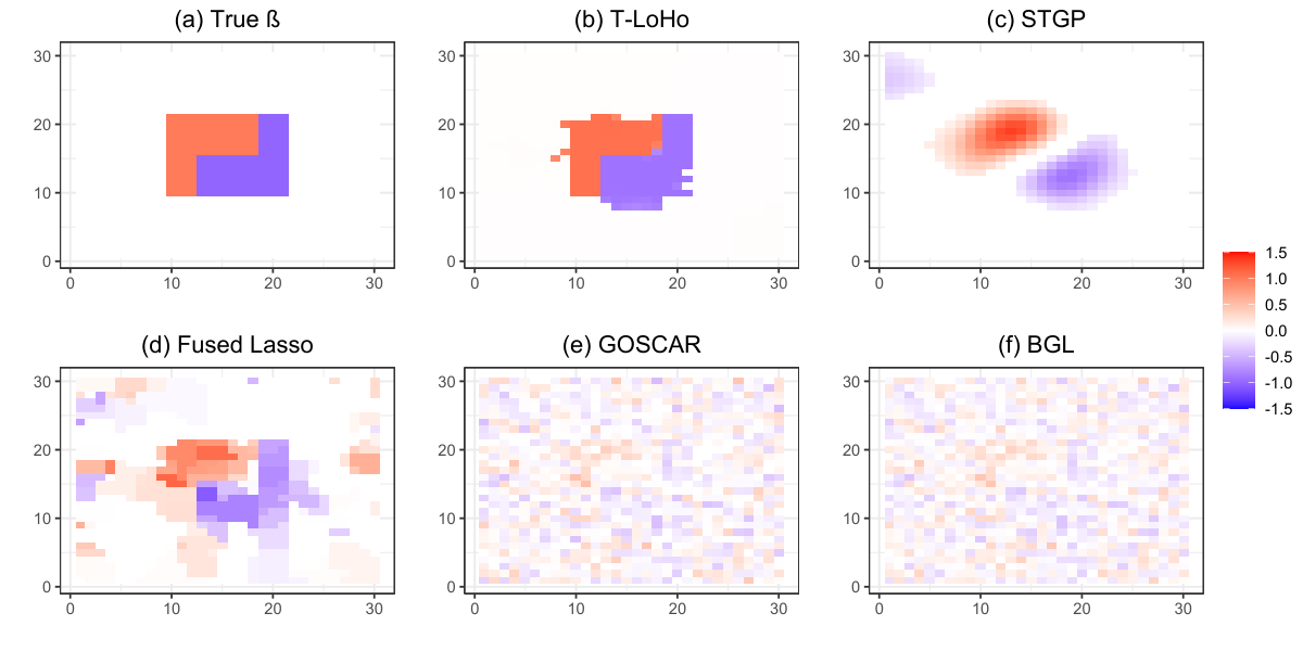
We conduct a simulation study to demonstrate the utility of our model. Motivated by the scalar-on-image regression problem, we consider a similar setting as Kang et al., 2018. We construct a $30\times 30$ lattice graph which represents a structure of 2-D image. Column-standardized image predictors $\mathbf{X}_{i}\in\mathbb{R}^{900},i=1,\ldots,100$ are generated from mean zero Gaussian process with kernel $K(x_{j},x_{l})=\exp(-d_{jl}/\vartheta)$ where $d_{jl}$ is the distance between pixels $j$ and $l$, $\vartheta$ is the range parameter with $\vartheta=0$ indicating no dependence. True coefficient $\bm{\beta}\in\mathbb{R}^{900}$ is sparse ($84\%$ are zero) and has irregular cluster shapes with sharp discontinuities as shown in fig. 4(a). We let $\text{SNR}\in\{2,4\}$ to set error variance $\sigma^{2}=\operatorname{Var}(\mathbf{X}\bm{\beta})/\text{SNR}$ and generate scalar responses $\bm{y}\in\mathbb{R}^{100}$ by $\bm{y}\sim\mathcal{N}(\mathbf{X}\bm{\beta},\sigma^{2}\mathbf{I})$.

We compared our model with the soft-thresholded Gaussian process (Kang et al., 2018, STGP,), sparse fused lasso on graph (Tibshirani et al., 2011; Wang et al., 2016, FL,), graph OSCAR  (Yang et al., 2012, GOSCAR,), and Bayesian graph Laplacian  (Chakraborty and Lozano, 2019, BGL,). We used mean squared prediction error (MSPE) with test set size 1000 to measure the predictive power and Rand index (RI) (Rand, 1971) to measure the clustering accuracy. For T-LoHo and STGP, we collected 4,000 posterior samples after 10,000 burn-in with 10 thin-in rate. For T-LoHo, we calculated the posterior median estimate of $\bm{\beta}$ and the cluster point estimate of $\Pi$ using Dahl, 2006’s method. For STGP, posterior mean estimate of $\bm{\beta}$ is used, and Rand index is calculated based on the binary classification (zero/non-zero) using posterior thresholding probabilities. For FL, the two tuning parameters are selected among the fixed candidate set of tuning parameter ratio $\gamma_{FL}\in\{0.2,1,5\}$ using the Bayesian information criterion. The T-LoHo and FL results presented here are when $(\tau_{0},c)=(1,0.5)$ and $\gamma_{FL}=0.2$ respectively; the hyperparameter sensitivity analysis of T-LoHo and the detailed settings of other models are available in Appendix A5. All computations were performed on Intel E5-2690 v3 CPU with 128GB of memory.

From fig. 4, we can see that T-LoHo successfully captures the irregular shape of cluster boundaries and sharp discontinuities. STGP gives a much more smoothed estimate (which is expected because it does not assume homogeneity), and FL estimate contains many falsely identified non-zero clusters. The superior performance of T-LoHo over FL is partly attributed to (i) the use of horseshoe that reduces bias in FL, and (ii) the use of RSF-based prior which more efficiently searches non-zero edge differences from a spanning forest instead of a full graph $G$ used in FL. Table 1 shows that in all ($\vartheta$,SNR) settings, T-LoHo indeed outperforms other models in terms of both predictive and clustering accuracy. GOSCAR and BGL give very similar results as their penalty functions have similar octagonal shapes, and both perform poorly in prediction and result in partitions with (nearly) all singletons. It is partly because GOSCAR and BGL allow the coefficients within the same cluster having similar magnitudes but with different signs. Additional simulation studies with more non-zero clusters are available in Appendix A5.

We applied T-LoHo to the problem of detecting anomalies in road graphs. NYC Pride March is an annual event held in every June in Manhattan, New York. As the march causes traffic congestion along the route, Wang et al., 2016 considered the problem of detecting clusters on the Manhattan road network which have different taxi pickup/dropoff patterns from usual. We constructed the road network graph using GRASS GIS (GRASS Development Team, 2020) and got 3748 nodes (junctions) and 8474 edges (sections of roads). Following Wang et al., 2016, we considered the event held in 2011 (12:00–2:00 pm, June 26th) and processed the number of taxi pickup/dropoff counts data¹¹ 1 Publicly available from NYC Taxi & Limousine Commission website, CC0. to the nearest nodes with log transformation. A log baseline seasonal average was calculated from the same time block 12:00–2:00 pm on the same day of the week across the nearest 8 weeks. Then it is plausible to assume that the difference between log counts on event day and log baseline seasonal average has many zeros and clustered patterns over the graph.

We fit T-LoHo and FL and compare the results. For T-LoHo, $(\tau_{0},c)=(1,0.8)$ were used to collect $5000$ posterior samples after $1.5\times 10^{5}$ burn-in with $10$ thin-in rate. For the FL estimate, we followed Wang et al., 2016’s specification where the regularizaton parameter in the fused term was chosen such that the model has 200 degrees of freedom and the one in the sparsity term is set as 0.2.

Figure 5 shows the fitted results of two models. Both successfully capture the decreased taxi activity along the parade route and slightly increased taxi activity around the starting/ending point of the parade. From the subplots, we can see that FL is biased because of soft-thresholding (Rinaldo et al., 2009) while T-LoHo appears to be less biased and capable of producing reasonable uncertainty measures. A notable difference is T-LoHo can capture the decreased taxi activity around the lower Manhattan area while FL cannot due to the bias. In summary, T-LoHo gives better insight on how taxi activity changes when such event occurs.

References

- Banerjee, (2021) Banerjee, S. (2021). Horseshoe shrinkage methods for Bayesian fusion estimation. arXiv preprint arXiv:2102.07378.
- Banerjee and Shen, (2020) Banerjee, S. and Shen, W. (2020). Graph signal denoising using -shrinkage priors. arXiv preprint arXiv:2012.13696.
- Berger et al., (1980) Berger, J. et al. (1980). A robust generalized bayes estimator and confidence region for a multivariate normal mean. Annals of Statistics, 8(4):716–761.
- Bhadra et al., (2019) Bhadra, A., Datta, J., Polson, N. G., Willard, B., et al. (2019). Lasso meets horseshoe: A survey. Statistical Science, 34(3):405–427.
- Carvalho et al., (2010) Carvalho, C. M., Polson, N. G., and Scott, J. G. (2010). The horseshoe estimator for sparse signals. Biometrika, 97(2):465–480.
- Chakraborty and Lozano, (2019) Chakraborty, S. and Lozano, A. C. (2019). A graph laplacian prior for bayesian variable selection and grouping. Computational Statistics & Data Analysis, 136:72–91.
- Dahl, (2006) Dahl, D. B. (2006). Model-based clustering for expression data via a dirichlet process mixture model. Bayesian inference for gene expression and proteomics, 4:201–218.
- Fan and Guan, (2018) Fan, Z. and Guan, L. (2018). Approximate -penalized estimation of piecewise-constant signals on graphs. The Annals of Statistics, 46(6B):3217–3245.
- Feng et al., (2016) Feng, W., Lim, C. Y., Maiti, T., and Zhang, Z. (2016). Spatial regression and estimation of disease risks: A clustering-based approach. Statistical Analysis and Data Mining: The ASA Data Science Journal, 9(6):417–434.
- George and McCulloch, (1993) George, E. I. and McCulloch, R. E. (1993). Variable selection via gibbs sampling. Journal of the American Statistical Association, 88(423):881–889.
- George and McCulloch, (1997) George, E. I. and McCulloch, R. E. (1997). Approaches for Bayesian variable selection. Statistica sinica, pages 339–373.
- Golub and Van Loan, (2013) Golub, G. H. and Van Loan, C. F. (2013). Matrix computations, volume 3. JHU press.
- Gönen et al., (2005) Gönen, M., Johnson, W. O., Lu, Y., and Westfall, P. H. (2005). The Bayesian two-sample t test. The American Statistician, 59(3):252–257.
- GRASS Development Team, (2020) GRASS Development Team (2020). Geographic Resources Analysis Support System (GRASS GIS) Software. Open Source Geospatial Foundation, USA.
- Green, (1995) Green, P. J. (1995). Reversible jump markov chain monte carlo computation and Bayesian model determination. Biometrika, 82(4):711–732.
- Guhaniyogi and Dunson, (2015) Guhaniyogi, R. and Dunson, D. B. (2015). Bayesian compressed regression. Journal of the American Statistical Association, 110(512):1500–1514.
- Hastie et al., (2015) Hastie, T., Tibshirani, R., and Wainwright, M. (2015). Statistical learning with sparsity: the lasso and generalizations. CRC press.
- Johndrow et al., (2020) Johndrow, J. E., Orenstein, P., and Bhattacharya, A. (2020). Scalable approximate mcmc algorithms for the horseshoe prior. Journal of Machine Learning Research, 21(73):1–61.
- Kang et al., (2018) Kang, J., Reich, B. J., and Staicu, A.-M. (2018). Scalar-on-image regression via the soft-thresholded Gaussian process. Biometrika, 105(1):165–184. code available at https://www4.stat.ncsu.edu/˜bjreich/software.
- Kass and Raftery, (1995) Kass, R. E. and Raftery, A. E. (1995). Bayes factors. Journal of the american statistical association, 90(430):773–795.
- Kass and Wasserman, (1995) Kass, R. E. and Wasserman, L. (1995). A reference bayesian test for nested hypotheses and its relationship to the schwarz criterion. Journal of the american statistical association, 90(431):928–934.
- Ke et al., (2015) Ke, Z. T., Fan, J., and Wu, Y. (2015). Homogeneity Pursuit. Journal of the American Statistical Association, 110(509):175–194.
- Kim and Gao, (2020) Kim, Y. and Gao, C. (2020). Bayesian model selection with graph structured sparsity. Journal of Machine Learning Research, 21(109):1–61.
- Knorr-Held and Raßer, (2000) Knorr-Held, L. and Raßer, G. (2000). Bayesian detection of clusters and discontinuities in disease maps. Biometrics, 56(1):13–21.
- Kyung et al., (2010) Kyung, M., Gill, J., Ghosh, M., Casella, G., et al. (2010). Penalized regression, standard errors, and Bayesian lassos. Bayesian Analysis, 5(2):369–411.
- Li and Sang, (2019) Li, F. and Sang, H. (2019). Spatial homogeneity pursuit of regression coefficients for large datasets. Journal of the American Statistical Association, 114(527):1050–1062.
- Liang et al., (2008) Liang, F., Paulo, R., Molina, G., Clyde, M. A., and Berger, J. O. (2008). Mixtures of g priors for Bayesian variable selection. Journal of the American Statistical Association, 103(481):410–423.
- Luo et al., (2021) Luo, Z. T., Sang, H., and Mallick, B. (2021). A Bayesian contiguous partitioning method for learning clustered latent variables. Journal of Machine Learning Research, 22(37):1–52.
- Neal, (2003) Neal, R. M. (2003). Slice sampling. Annals of statistics, pages 705–741.
- Padilla et al., (2017) Padilla, O. H. M., Sharpnack, J., Scott, J. G., and Tibshirani, R. J. (2017). The DFS fused lasso: Linear-time denoising over general graphs. J. Mach. Learn. Res., 18:176–1.
- Polson and Scott, (2010) Polson, N. G. and Scott, J. G. (2010). Shrink globally, act locally: Sparse Bayesian regularization and prediction. Bayesian statistics, 9(501-538):105.
- Polson et al., (2014) Polson, N. G., Scott, J. G., and Windle, J. (2014). The Bayesian bridge. Journal of the Royal Statistical Society: Series B: Statistical Methodology, pages 713–733.
- Rand, (1971) Rand, W. M. (1971). Objective criteria for the evaluation of clustering methods. Journal of the American Statistical association, 66(336):846–850.
- Rinaldo et al., (2009) Rinaldo, A. et al. (2009). Properties and refinements of the fused lasso. Annals of Statistics, 37(5B):2922–2952.
- Rue, (2001) Rue, H. (2001). Fast sampling of Gaussian markov random fields. Journal of the Royal Statistical Society: Series B (Statistical Methodology), 63(2):325–338.
- Shimamura et al., (2019) Shimamura, K., Ueki, M., Kawano, S., and Konishi, S. (2019). Bayesian generalized fused lasso modeling via neg distribution. Communications in Statistics-Theory and Methods, 48(16):4132–4153.
- Shin et al., (2020) Shin, M., Bhattacharya, A., and Johnson, V. E. (2020). Functional horseshoe priors for subspace shrinkage. Journal of the American Statistical Association, 115(532):1784–1797.
- Song and Cheng, (2020) Song, Q. and Cheng, G. (2020). Bayesian fusion estimation via t shrinkage. Sankhya A, 82(2):353–385.
- Strawderman, (1971) Strawderman, W. E. (1971). Proper bayes minimax estimators of the multivariate normal mean. The Annals of Mathematical Statistics, 42(1):385–388.
- Tang and Song, (2016) Tang, L. and Song, P. X. (2016). Fused lasso approach in regression coefficients clustering: learning parameter heterogeneity in data integration. The Journal of Machine Learning Research, 17(1):3915–3937.
- Teixeira et al., (2019) Teixeira, L. V., Assunção, R. M., and Loschi, R. H. (2019). Bayesian space-time partitioning by sampling and pruning spanning trees. Journal of Machine Learning Research, 20(85):1–35.
- Tibshirani et al., (2005) Tibshirani, R., Saunders, M., Rosset, S., Zhu, J., and Knight, K. (2005). Sparsity and smoothness via the fused lasso. Journal of the Royal Statistical Society: Series B (Statistical Methodology), 67(1):91–108.
- Tibshirani et al., (2011) Tibshirani, R. J., Taylor, J., et al. (2011). The solution path of the generalized lasso. The Annals of Statistics, 39(3):1335–1371.
- Wang et al., (2016) Wang, Y.-X., Sharpnack, J., Smola, A. J., and Tibshirani, R. J. (2016). Trend filtering on graphs. Journal of Machine Learning Research, 17(105):1–41.
- Yang et al., (2012) Yang, S., Yuan, L., Lai, Y.-C., Shen, X., Wonka, P., and Ye, J. (2012). Feature grouping and selection over an undirected graph. In Proceedings of the 18th ACM SIGKDD international conference on Knowledge discovery and data mining, pages 922–930.
- Zhu et al., (2013) Zhu, Y., Shen, X., and Pan, W. (2013). Simultaneous grouping pursuit and feature selection over an undirected graph. Journal of the American Statistical Association, 108(502):713–725.