Metapopulation dynamics of a respiratory disease with infection during travel

Indrajit Ghosh Note: Corresponding author. Email: indra7math@gmail.com Address: Department of Computational and Data Sciences, Indian Institute of Science, Bengaluru-560012, Karnataka, India Sk Shahid Nadim Address: Agricultural and Ecological Research Unit, Indian Statistical Institute, Kolkata - 700 108, West Bengal, India Soumyendu Raha Address: Department of Computational and Data Sciences, Indian Institute of Science, Bengaluru-560012, Karnataka, India Debnath Pal Address: Department of Computational and Data Sciences, Indian Institute of Science, Bengaluru-560012, Karnataka, India

Abstract

We formulate a compartmental model for the propagation of a respiratory disease in a patchy environment. The patches are connected through the mobility of individuals, and we assume that disease transmission and recovery are possible during travel. Moreover, the migration terms are assumed to depend on the distance between patches and the perceived severity of the disease. The positivity and boundedness of the model solutions are discussed. We analytically show the existence and global asymptotic stability of the disease-free equilibrium. We study three different network topologies numerically and find that underlying network structure is crucial for disease transmission. Further numerical simulations reveal that infection during travel has the potential to change the stability of disease-free equilibrium from stable to unstable. The coupling strength and transmission coefficients are also very crucial in disease propagation. Different exit screening scenarios indicate that the patch with the highest prevalence may have adverse effects but other patches will be benefited from exit screening. Furthermore, while studying the multi-strain dynamics, it is observed that two co-circulating strains will not persist simultaneously in the community but only one of the strains may persist in the long run. Transmission coefficients corresponding to the second strain are very crucial and show threshold like behavior with respect to the equilibrium density of the second strain.

Keywords:

Epidemic model, Infection during travel, Metapopulation, Stability analysis, Numerical simulations

1 Introduction

Many epidemic outbreaks such as 1918 pandemic influenza, 2002-2003 SARS outbreak, 2009 H1N1 influenza epidemic, 2012 - 2015 MERS-CoV outbreak, 2015 Ebola virus epidemic and ongoing COVID-19 pandemic indicate that increasing connectivity has significantly amplified the impact of these diseases. Respiratory diseases such as TB, influenza, COVID-19, etc. are mainly caused by direct contact, indirect contact, respiratory droplets or airborne transmission. Direct contact refers to the human-to-human physical contact and indirect contact indicate contact through intermediate object such as door knob, sitting bench etc. Respiratory droplets are exhaled from infectious humans while sneezing or coughing. These droplets can then be deposited on a healthy human’s mucus or conjunctiva. Another transmission path is the airborne one which involves infectious pathogens travelling through air from an infected host to a healthy one brankston2007transmission; arino2016revisiting. However, pathogens may not only transmit within patches but also during travel. As during travel, individuals are put in a close proximity for a significant duration, it is highly likely that the probability of transmission increases with duration of transport or equivalently distance travelled. Therefore the infection during travel may be negligible in short-range transport but in the case of long-range transport infection during travel may have a significant impact. Transmission of respiratory diseases during travel has been reported in many instances. In a report by the European Centre for Disease prevention and Control stated that TB, measles and seasonal influenza are transmissible during commercial flights knipl2016stability. WHO confirmed influenza transmission during long distance train travels furuya2007risk. Mangili and Gendreau mangili2005transmission reviewed about transmission while travelling in aircraft, and infection spread within cars has also been studied knibbs2012risk. Consequently, the infection during travel is important to study. The specific impact of infection while traveling is not well understood. Specifically, in the case of pandemic outbreaks (for instance influenza, COVID-19 etc.) the virus is highly infectious and may intensify the overall disease burden if long-range travels are not supervised.

Mathematical modeling can shed light on the potential impact of infection during transportation on the global burden of respiratory illness. To analyze the transmission patterns of these diseases without infection during travel, various metapopulation models have been studied in the literature (see arino2017spatio; lloyd2004spatiotemporal; bahl2011temporally and references therein). Despite its importance, the consideration of infection during transport in these metapopulation models is not yet emerged as a very active research area. Previously, various authors considered single patch and inflow of infected individuals. A disease transmission model in a single patch with inflow of infectious agents was considered brauer2001models. Guo and coauthors investigated problems associated with the inflow of people infected with TB guo2011global. The problem has been discussed by some authors in the context of delay differential equations to incorporate precise travel time between patches liu2008modeling; nakata2011global; knipl2016stability. A few basic SIS (Susceptible-Infected-Susceptible) models (ordinary differential equation) are studied with infection during travel takeuchi2006spreading; takeuchi2007global; arino2016revisiting. Takeuchi and coauthors takeuchi2006spreading; takeuchi2007global presented SIS patch models with infection during transport. But they made a simplifying assumption that all model parameters are the same in both patches. However, Arino and coauthors arino2016revisiting modified an earlier model of Takeuchi and coauthors takeuchi2006spreading to allow all the parameters to be different in two patches. However, SIS-type models are inadequate for respiratory diseases with high infectiousness (eg. influenza, SARS, measles and COVID-19). For instance, respiratory diseases such as measles bolker1993chaos, COVID-19 wu2020nowcasting, tuberculosis liu2010tuberculosis, influenza A etbaigha2018seir were modelled using an SEIR (Susceptible-Exposed-Infected-Recovered) system. This indicate that SEIR type models are necessary to model these respiratory diseases. Therefore, we extend the metapopulation models to SEIR version theoretically. Due to the consideration of SEIR system, travel related recovery and incubation period are also important to model in this context. Another realistic modification will consider the migration rates depending on the distance between patches and perceived severity of the disease. To do so, we may assume the migration rates to be inversely proportional to the distance between patches and inversely proportional to the perceived severity of the disease. These two assumptions are realistic but they were not considered in the context of infection during travel. Moreover, respiratory diseases are prone to mutation and multiple strains often emerge in the population lyons2018mutation; garcia2021multiple. Thus, it is important to incorporate multi-strain dynamics in the model under investigation. Motivated by the above discussion, we study the dynamics of a metapopulation model with infection during travel in different scenarios.

The rest of the paper is organized as follows: in Sect. 2, the assumptions for the metapopulation model are stated and the corresponding model is formulated; in Sect. 3, some basic mathematical properties of the model are deduced; in Sect. 4, different numerical simulations are performed to get insight into the transmission dynamics and finally in Sect. 5, a brief discussion about the results is presented.

2 Model description

The following assumptions are made while formulating the model.

1.

We consider n disjoint patches with total populations $N_{i}$ , i=1,2,…,n. The total population in each patch are subdivided into four compartments namely, Susceptible ( $S$ ), Exposed ( $E$ ), Infected ( $I$ ) and Recovered ( $R$ ).
2.

There is homogeneous mixing between people. Within each patch standard incidence rate of disease transmission is occurring, i.e, force of infection = $\frac{\beta_{i}S_{i}I_{i}}{N_{i}}$ .
3.

Newly recruited people in each patch are susceptible in their respective patch. Individuals in each patch die at natural death rate. Disease induced death rate is considered only in compartments $I_{i}$ . Exposed people will progress to infectious compartment after an incubation period in each patch.
4.

During travel new infection take place at rate $\frac{\alpha_{j}m_{ij}S_{j}I_{j}}{N_{j}}$ , $m_{ij}$ is the rate of travel of each compartment from patch j to patch i arino2016revisiting.
5.

While travelling, exposed people may become infectious and infected people will also recover at certain rates.
6.

The migration rates between patches are assumed to be inversely proportional to the distance between patches as well as the perceived severity of the disease. Thus, $m_{ij}=\epsilon\frac{1}{d_{ij}^{\eta}\nu_{j}}$ , where $d_{ij}$ is the distance between patch i and patch j, $\eta$ governs the distance dependency of migration rate, $\nu_{j}\geq 1$ measure the perceived severity of the disease. Note that, when $\nu_{j}=1$ the migration rates do not depend on the disease severity.

The SEIR metapopulation model based on the above assumptions take take the following form

$\displaystyle\displaystyle{\frac{dS_{i}}{dt}}$	$\displaystyle=$	$\displaystyle\Pi_{i}-\beta_{i}\frac{I_{i}}{N_{i}}S_{i}-\mu_{i}S_{i}-\sum_{j=1}^{n}m_{ji}S_{i}+\sum_{j=1}^{n}m_{ij}(1-\frac{\alpha_{j}I_{j}}{N_{j}})S_{j},$
$\displaystyle\displaystyle{\frac{dE_{i}}{dt}}$	$\displaystyle=$	$\displaystyle\beta_{i}\frac{I_{i}}{N_{i}}S_{i}-(\gamma_{i}+\mu_{i})E_{i}-\sum_{j=1}^{n}m_{ji}E_{i}+\sum_{j=1}^{n}m_{ij}\frac{\alpha_{j}I_{j}}{N_{j}}S_{j}+\sum_{j=1}^{n}(1-\xi_{i})m_{ij}E_{j},$	(2.1)
$\displaystyle\displaystyle{\frac{dI_{i}}{dt}}$	$\displaystyle=$	$\displaystyle\gamma_{i}E_{i}-(\sigma_{i}+\mu_{i}+\delta_{i})I_{i}-\sum_{j=1}^{n}m_{ji}I_{i}+\sum_{j=1}^{n}\xi_{i}m_{ij}E_{j}+\sum_{j=1}^{n}(1-p_{i})m_{ij}I_{j},$
$\displaystyle\displaystyle{\frac{dR_{i}}{dt}}$	$\displaystyle=$	$\displaystyle\sigma_{i}I_{i}-\mu_{i}R_{i}-\sum_{j=1}^{n}m_{ji}R_{i}+\sum_{j=1}^{n}m_{ij}R_{j}+\sum_{j=1}^{n}p_{i}m_{ij}I_{j},$

where, $m_{ii}=m_{jj}=0$ and $m_{ij}=\epsilon\frac{1}{d_{ij}^{\eta}\nu_{j}}$ . A flow diagram of a source-destination patch version of model (2) is illustrated in Fig. 1.

Refer to caption — Figure 1: Flow chart of a source-destination version of SEIR metapopulation model with infection during travel. Solid black arrows depict usual progressions of a compartmental SEIR model and black arrows with fine dots are used to show migration of people. The black dashed arrow (2 dots 3 dashes) represents newly exposed persons during travel, the black dashed line represents the persons becoming infected from exposed and the black dashed line (2 dots one dash) represents the recovery during travel.

3 Mathematical analysis

3.1 Positivity and boundedness of the solution

This subsection is provided to prove the positivity and boundedness of solutions of the system (2) with initial conditions $(S_{i}(0),E_{i}(0),I_{i}(0),R_{i}(0))^{T}\in\mathbb{R}_{+}^{4n}$ .

Proposition 3.1.

The system (2) is positively invariant in $\mathbb{R}_{+}^{4n}$ .

Proof.

To demonstrate the solution’s positivity, it is sufficient to prove that each of the positive orthant’s faces cannot be crossed, implying that the vector field points inward on the boundary of $\mathbb{R}_{+}^{4n}$ .
By re-writing the system (2) we have

\displaystyle\frac{dX_{i}}{dt}

\displaystyle=F(X_{i}(t),X_{0}),X_{i0}\geq 0

(3.1)

$F(X_{i}(t))=(F_{1}(X_{i}),F_{2}(X_{i}),F_{3}(X_{i}),F_{4}(X_{i}))^{T}$
We note that

	$\displaystyle\frac{dS_{i}}{dt}\|_{S_{i}=0}$	$\displaystyle=\Pi_{i}+\sum_{j=1}^{n}m_{ij}(1-\frac{\alpha_{j}I_{j}}{N_{j}})\geq 0,$
	$\displaystyle\frac{dE_{i}}{dt}\|_{E_{i}=0}$	$\displaystyle=\beta_{i}\frac{I_{i}}{N_{i}}S_{i}+\sum_{j=1}^{n}m_{ij}\frac{\alpha_{j}I_{j}}{N_{j}}S_{j}+\sum_{j=1}^{n}(1-\xi_{i})m_{ij}E_{j}\geq 0,$
	$\displaystyle\frac{dI_{i}}{dt}\|_{I_{i}=0}$	$\displaystyle=\gamma_{i}E_{i}+\sum_{j=1}^{n}\xi_{i}m_{ij}E_{j}+\sum_{j=1}^{n}(1-p_{i})m_{ij}I_{j}\geq 0,$
	$\displaystyle\frac{dR_{i}}{dt}\|_{R_{i}=0}$	$\displaystyle=\sigma_{i}I_{i}+\sum_{j=1}^{n}m_{ij}R_{j}+\sum_{j=1}^{n}p_{i}m_{ij}I_{j}\geq 0.$

Then it follows from Theorem 3.1 of Sun et al. sun2011effect that all the $4n$ state variables remain non-negative for all time. Hence, $\mathbb{R}_{+}^{4n}$ is a positively invariant set for the system (2). ∎

Proposition 3.2.

The solutions $(S_{i}(t),E_{i}(t),I_{i}(t),R_{i}(t))$ of the model (2) are ultimately and uniformly bounded in $\mathbb{R}_{+}^{4n}$ .

Proof.

Let $N_{i}(t)=S_{i}(t)+E_{i}(t)+I_{i}(t)+R_{i}(t)$ be the entire human population at time $t$ in patch $i$ and in all patches, $N=\sum_{i=1}^{n}N_{i}$ be the entire population. Also we define $\Pi=\sum_{i=1}^{n}\Pi_{i}$ and $\mu=min_{1\leq i\leq n}\mu_{i}$ .
Now adding $4n$ equations we have

\displaystyle\frac{dN_{i}}{dt}=\Pi_{i}-\mu_{i}N_{i}-\delta_{i}I_{i}-\sum_{X=S,E,I,R}\Big(\sum_{j=1}^{n}m_{ji}X_{i}-\sum_{j=1}^{n}m_{ij}X_{j}\Big)

Now, if we add $i$ from $1$ to $n$ , we have,

\displaystyle\frac{dN}{dt}=\sum_{i=1}^{n}\Big[\Pi_{i}-\mu_{i}N_{i}-\delta_{i}I_{i}-\sum_{X=S,E,I,R}\Big(\sum_{j=1}^{n}m_{ji}X_{i}-\sum_{j=1}^{n}m_{ij}X_{j}\Big)\Big]

In the preceding equation, the double summation is vanished and since $I_{i}\leq N_{i}$ , it follows that

	$\displaystyle\frac{dN}{dt}$	$\displaystyle\leq\sum_{i=1}^{n}\Pi_{i}-\sum_{i=1}^{n}\mu_{i}N_{i}$
		$\displaystyle\leq\sum_{i=1}^{n}\Pi_{i}-\sum_{i=1}^{n}min_{1\leq i\leq n}\mu_{i}N_{i}$

Hence by standard comparison theorem,

\displaystyle N(t)\leq\Big\{\frac{\sum_{i=1}^{n}\Pi_{i}}{\sum_{i=1}^{n}min_{1\leq i\leq n}\mu_{i}}\Big\}\Longrightarrow N(t)\leq\frac{\Pi}{\mu}

Therefore the solutions of the model (2) are ultimately and uniformly bounded in $\mathbb{R}_{+}^{4n}$ . ∎

Corollary 3.1.

The region $\Omega=\{(S_{i},E_{i},I_{i},R_{i})\in\mathbb{R}_{+}^{4n}|N\leq\frac{\Pi}{\mu}\}$ is invariant and attracting for system (2).

3.2 Stability of disease-free equilibrium and basic reproduction number

Let $M=[m_{ij}]$ be the travel rate matrix for each compartments, is assumed to be irreducible. The matrix $M$ represents the human movement among patches.

Define $n\times n$ matrices

\displaystyle\psi^{X}=\text{diag}(\mu_{i}^{X}+\sum_{j=1}^{n}m_{ji})-M

where, $\mu_{i}^{S}=\mu_{i}$ , $\mu_{i}^{E}=\gamma_{i}+\mu_{i}$ , $\mu_{i}^{I}=\sigma_{i}+\delta_{i}+\mu_{i}$ and $\mu_{i}^{R}=\mu_{i}$ .

For example,

\displaystyle\psi^{R}=\begin{bmatrix}\mu_{1}+\sum_{j=1}^{n}m_{j1}&-m_{12}&\cdots&-m_{1n}\\ -m_{21}&\mu_{2}+\sum_{j=1}^{n}m_{j2}&\cdots&-m_{2n}\\ \vdots&\vdots&\ddots&\vdots\\ -m_{n1}&-m_{n2}&\cdots&\mu_{n}+\sum_{j=1}^{n}m_{jn}\\ \end{bmatrix}

(3.2)

The matrices above are non-singular M-matrices since all off-diagonal entries are nonpositive (i.e., of the Z-sign pattern) and the sum of the entries in each column is positive and $\psi^{{X}}\geq 0$ berman1994nonnegative, where $X=S,E,I,R$ . The phase at which no disease exists in the population is referred to as disease free equilibrium (DFE). For this we set $E_{i}=0,I_{i}=0$ in the equation (2). Then the system of equation (2) reduces to:

	$\displaystyle\displaystyle{\frac{dS_{i}}{dt}}$	$\displaystyle=$	$\displaystyle\Pi_{i}-\mu_{i}S_{i}-\sum_{j=1}^{n}m_{ji}S_{i}+\sum_{j=1}^{n}m_{ij}S_{j},$		(3.3)
	$\displaystyle\displaystyle{\frac{dR_{i}}{dt}}$	$\displaystyle=$	$\displaystyle-\mu_{i}R_{i}-\sum_{j=1}^{n}m_{ji}R_{i}+\sum_{j=1}^{n}m_{ij}R_{j},$

We take the following equations to calculate the DFE:

	$\displaystyle 0$	$\displaystyle=$	$\displaystyle\Pi_{i}-\mu_{i}S_{i}-\sum_{j=1}^{n}m_{ji}S_{i}+\sum_{j=1}^{n}m_{ij}S_{j},$		(3.4)
	$\displaystyle 0$	$\displaystyle=$	$\displaystyle-\mu_{i}R_{i}-\sum_{j=1}^{n}m_{ji}R_{i}+\sum_{j=1}^{n}m_{ij}R_{j},$

This can be expressed as a matrix form:

	$\displaystyle\psi^{S}S$	$\displaystyle=\Pi_{i}$		(3.5)
	$\displaystyle\psi^{R}R$	$\displaystyle=0$

where, $\psi^{S}=\text{diag}(\mu_{i}+\sum_{j=1}^{n}m_{ji})-M$ , $\psi^{R}=\text{diag}(\mu_{i}+\sum_{j=1}^{n}m_{ji})-M$ , $M$ is an irreducible movement matrix and $S=(S_{1},S_{2},......,S_{n})^{T}$ , $R=(R_{1},R_{2},......,R_{n})^{T}$ , $\Pi=(\Pi_{1},\Pi_{2},......,\Pi_{n})^{T}$ .

We can see that the matrices $\psi^{S}$ and $\psi^{R}$ have non-positive off-diagonal components and the total sum of each column’s entries is positive. As a result, both $\psi^{S}$ and $\psi^{R}$ are non-singular M-matrices and have positive inverses berman1994nonnegative. As a consequence, the second equation of (3.4) has trivial solution, while the first equation of (3.4) has a unique positive solution $S^{0}=(S_{1}^{0},S_{2}^{0},......,S_{n}^{0})=(\psi^{S})^{-1}\Pi$ .

As a consequence, we get the following result.

Theorem 3.1.

There exits a DFE $P^{0}=(S_{1}^{0},0,0,0,S_{2}^{0},0,0,0,....,S_{n}^{0},0,0,0)\in\mathbb{R}_{+}^{4n}$ for the system (2) which is unique.

3.2.1 Basic Reproduction Number

The system (2) has a unique disease-free equilibrium (DFE) and is given by

\displaystyle P^{0}=(S_{1}^{0},0,0,0,S_{2}^{0},0,0,0,....,S_{n}^{0},0,0,0)\in\mathbb{R}_{+}^{4n}.

Following senapati2019cholera, the matrix $(F)$ of new infection and the matrix $(V)$ of transition terms are given below:

\displaystyle F=\begin{bmatrix}\begin{array}[]{cc}0&F_{11}\\ 0&0\\ \end{array}\end{bmatrix}\text{ and }V=\begin{bmatrix}\begin{array}[]{cc}V_{11}&0\\ -V_{21}&V_{22}\\ \end{array}\end{bmatrix}

where,

	$\displaystyle F_{11}$	$\displaystyle=\begin{bmatrix}\beta_{1}&m_{12}\alpha_{2}&m_{13}\alpha_{3}&\cdots&m_{1n}\alpha_{n}\\ m_{21}\alpha_{1}&\beta_{2}&m_{23}\alpha_{3}&\cdots&m_{2n}\alpha_{n}\\ \vdots&\vdots&\vdots&\ddots&\vdots\\ m_{n1}\alpha_{1}&m_{n2}\alpha_{2}&m_{n3}\alpha_{3}&\cdots&\beta_{n}\\ \end{bmatrix}$
	$\displaystyle V_{11}$	$\displaystyle=\begin{bmatrix}(\gamma_{1}+\mu_{1})+\sum_{j=1}^{n}m_{j1}&-(1-\xi_{1})m_{12}&\cdots&-(1-\xi_{1})m_{1n}\\ -(1-\xi_{2})m_{21}&(\gamma_{2}+\mu_{2})+\sum_{j=1}^{n}m_{j2}&\cdots&-(1-\xi_{2})m_{2n}\\ \vdots&\vdots&\ddots&\vdots\\ -(1-\xi_{n})m_{n1}&-(1-\xi_{n})m_{n2}&\cdots&(\gamma_{n}+\mu_{n})+\sum_{j=1}^{n}m_{jn}\\ \end{bmatrix}$
	$\displaystyle V_{21}$	$\displaystyle=\begin{bmatrix}\gamma_{1}&\xi_{1}m_{12}&\cdots&\xi_{1}m_{1n}\\ \xi_{2}m_{21}&\gamma_{2}&\cdots&\xi_{2}m_{2n}\\ \vdots&\vdots&\ddots&\vdots\\ \xi_{n}m_{n1}&\xi_{n}m_{n2}&\cdots&\gamma_{n}\\ \end{bmatrix}$
	$\displaystyle V_{22}$	$\displaystyle=\begin{bmatrix}(\sigma_{1}+\mu_{1}+\delta_{1})+\sum_{j=1}^{n}m_{j1}&-(1-p_{1})m_{12}&\cdots&-(1-p_{1})m_{1n}\\ -(1-p_{2})m_{21}&(\sigma_{2}+\mu_{2}+\delta_{2})+\sum_{j=1}^{n}m_{j2}&\cdots&-(1-p_{2})m_{2n}\\ \vdots&\vdots&\ddots&\vdots\\ -(1-p_{n})m_{n1}&-(1-p_{n})m_{n2}&\cdots&(\sigma_{n}+\mu_{n}+\delta_{n})+\sum_{j=1}^{n}m_{jn}\\ \end{bmatrix}$

From the above we have seen that $F\geq 0$ and the Z-sign pattern is present in $V$ . Since

\displaystyle V^{-1}=\begin{bmatrix}\begin{array}[]{cc}V_{11}^{-1}&0\\ V_{22}^{-1}V_{21}V_{11}^{-1}&V_{22}^{-1}\\ \end{array}\end{bmatrix}\geq 0,

V is a irreducible nonsingular M-matrix. Following van2002reproduction, the basic reproduction number, denoted by $R_{0}$ is the spectral radius of the next generation matrix $FV^{-1}$ , where,

\displaystyle FV^{-1}=\begin{bmatrix}\begin{array}[]{cc}0&F_{11}\\ 0&0\\ \end{array}\end{bmatrix}\begin{bmatrix}\begin{array}[]{cc}V_{11}^{-1}&0\\ V_{22}^{-1}V_{21}V_{11}^{-1}&V_{22}^{-1}\\ \end{array}\end{bmatrix}

Therefore,

\displaystyle R_{0}=\rho(FV^{-1})=\rho(F_{11}V_{22}^{-1}V_{21}V_{11}^{-1})

(3.6)

where $\rho(X)$ represents the spectral radius of the matrix $X$ .

To indicate that the expression for $R_{0}$ is dependent on the whole network, we refer to it as the domain basic reproduction number. According to Theorem 2 in van2002reproduction that the DFE of the model (2) is locally asymptotically stable whenever $R_{0}<1$ , while unstable if $R_{0}>1$ .

In the specific case of $n=1$ , the basic reproduction number has the explicit form

\displaystyle R_{0}=\frac{\beta\gamma}{(\gamma+\mu)(\sigma+\mu+\delta)}

In the special case of no humans migrate between patches (i.e., $M=0$ ), the basic reproduction number $R_{0}$ defined in 3.6 is represented by the maximum possible value of basic reproduction numbers $R_{0}$ in every patches. Therefore, $R_{0}=\max\limits_{i}\{R_{0}^{(i)}\}$
where

\displaystyle R_{0}^{(i)}=\frac{\beta_{i}\gamma_{i}}{(\gamma_{i}+\mu_{i})(\sigma_{i}+\mu_{i}+\delta_{i})}\text{ i=1,2,\ldots,n}

(3.7)

3.2.2 Bounds on $R_{0}$

Let there is no human movements, i.e., $M=0$ . Also let us assume that $\beta_{i}=\beta$ , $\gamma_{i}=\gamma$ , $\gamma_{i}+\mu_{i}=\gamma+\mu$ and $\sigma_{i}+\mu_{i}+\delta_{i}=\sigma+\mu+\delta$ for all $i$ . Then,

\displaystyle R_{0}=\frac{1}{\gamma+\mu}\rho(F_{11}V_{22}^{-1}V_{21})

From spectral properties of non-negative matrices, $R_{0}$ can be bounded above and below.

Theorem 3.2.

Assume that $\beta_{i}=\beta$ , $\gamma_{i}=\gamma$ , $\gamma_{i}+\mu_{i}=\gamma+\mu$ and $\sigma_{i}+\mu_{i}+\delta_{i}=\sigma+\mu+\delta$ for all $i$ and $M^{E}=M^{I}=0$ . Then

\displaystyle\min\limits_{i}\{R_{0}^{(i)}\}\leq R_{0}\leq\max\limits_{i}\{R_{0}^{(i)}\}.

Proof.

The proof is motivated by similar outcomes in hsieh2007impact; salmani2006model and the fact that $F_{11}V_{22}^{-1}V_{21}$ is similar to $V_{21}F_{11}V_{22}^{-1}$ . Let $V_{22}^{-1}=Y=[y_{ij}]$ , $\textbf{1}=(1,1,\dots,1)^{T}\in\mathbb{R}^{n}$ and $[1^{T}V_{21}F_{11}V_{22}^{-1}]_{i}$ denote the sum of each entries in the $i^{th}$ column of $V_{21}F_{11}V_{22}^{-1}$ . Since the column sum of $V_{22}$ is $(\sigma+\mu+\delta)$ , $\textbf{1}^{T}V_{22}=(\sigma+\mu+\delta)\textbf{1}^{T}$ , giving $\textbf{1}^{T}Y=\frac{1}{\sigma+\mu+\delta}\textbf{1}^{T}$ . Therefore, the column sum of $Y$ is $\frac{1}{\sigma+\mu+\delta}$ . Then

	$\displaystyle[1^{T}V_{21}F_{11}V_{22}^{-1}]$	$\displaystyle=\beta_{1}\gamma_{1}y_{1i}+\beta_{2}\gamma_{2}y_{2i}+\dots+\beta_{n}\gamma_{n}y_{ni}$
		$\displaystyle\leq\max\limits_{i}\{{\beta_{i}\gamma_{i}}\}(y_{1i}+y_{2i}+\dots+y_{ni})$
		$\displaystyle=\max\limits_{i}\Big\{\frac{\beta_{i}\gamma_{i}}{\sigma+\mu+\delta}\Big\}.$

Similarly, $[1^{T}V_{21}F_{11}V_{22}^{-1}]\geq\min\limits_{i}\Big\{\frac{\beta_{i}\gamma_{i}}{\sigma+\mu+\delta}\Big\}.$
The conclusion follows from the facts that $\rho(F_{11}V_{22}^{-1}V_{21})$ lies between its minimum and maximum column sums and that $R_{0}=\rho(V_{22}^{-1}V_{21}F_{11})=\rho(F_{11}V_{22}^{-1}V_{21})$ . ∎

3.2.3 Global stability of disease-free equilibrium

Theorem 3.3.

Assume that the movement matrix $M$ is irreducible. Then the following results exhibit for the model (2)
(1) If $R_{0}<1$ , then the disease-free equilibrium (DFE) $P^{0}$ of (2) is globally asymptotically stable in the region $\Omega$ .
(2) If $R_{0}>1$ , then the disease-free equilibrium (DFE) $P^{0}$ of (2) is unstable and the model (2) is uniformly persistent.

Proof.

To prove the above theorem, we follow the following procedure as in the proof of Theorem 5.1 in eisenberg2013cholera.

Let us define $x=(E_{1},E_{2},....,E_{n},I_{1},I_{2},.....,I_{n})$ . Following Exercise 1.2, in johnson1985matrix, the matrices $FV^{-1}$ and $V^{-1}F$ have the same spectral radius. Thus $R_{0}=\rho(V^{-1}F)=\rho(FV^{-1})$ . Assume that $b$ is the left eigenvector of $V^{-1}F$ , which corresponds to the eigenvalue $R_{0}$ . This implies $b^{T}V^{-1}F=R_{0}b^{T}$ .

Let us consider the following Lyapunov function

\displaystyle L=(b^{T}V^{-1}x)

(3.8)

Differentiating $L$ along (2) gives,

$\displaystyle L^{\prime}$	$\displaystyle=b^{T}V^{-1}x^{\prime}$
	$\displaystyle\leq b^{T}V^{-1}(F-V)x$
	$\displaystyle=b^{T}V^{-1}Fx-b^{T}x$
	$\displaystyle=(R_{0}-1)b^{T}x\leq 0,\text{ if }R_{0}<1.$	(3.9)

Using the irreducibility of the matrix $M$ , it can be checked that the singleton $\{P^{0}\}$ is the unique invariant set where $L^{\prime}=0$ . Therefore by using LaSalle’s invariance principle la1976stability, $P^{0}$ is globally asymptotically stable in $\Omega$ .

Alternatively, if $R_{0}>1$ and $x>0$ , it follows that $(R_{0}-1)b^{T}x>0$ . This combination of inequality and continuity imply that $L^{\prime}>0$ for a small neighborhood of $P^{0}$ in int( $\Omega$ ). That is, for $R_{0}>1$ , any solution which is sufficiently close to $P^{0}$ will step away from $P^{0}$ . Based on the results of li1999global, and using the irreducibility of the matrix $M$ , the instability of $P^{0}$ indicates the uniform persistence of the model (2). ∎

4 Numerical simulations

We consider the infection is originated in patch 1 i.e, few people are infected in patch 1 while other patches have no infection in the beginning. Initial conditions are $(S_{1}(0),E_{1}(0),I_{1}(0),R_{1}(0))=(100000,100,10,0)$ and $(S_{i}(0),E_{i}(0),I_{i}(0),R_{i}(0))=(100000,0,0,0)$ for i=2,3,4,5. Some fixed parameters are reported in Table 1 and some other fixed parameters are $d_{12}=d_{21}=100$ , $d_{13}=d_{31}=110$ , $d_{14}=d_{41}=120$ , $d_{15}=d_{51}=130$ , $d_{23}=d_{32}=140$ , $d_{24}=d_{42}=150$ , $d_{25}=d_{52}=160$ , $d_{34}=d_{43}=170$ , $d_{35}=d_{53}=180$ , $d_{45}=d_{54}=190$ and $(\nu_{1},\nu_{2},\nu_{3},\nu_{4},\nu_{5})=(7,6,5,4,3)$ . These parameters are kept constant throughout the numerical simulation section.

Table 1: Parameter values and their units used in the numerical simulation

Parameter	value/Range	unit
$\mu_{i}$	0.00032	week^-1
$\Pi_{i}$	$N_{i}\times\mu_{i}$	Person week^-1
$\beta_{i}$	(0,1)	week^-1
$\alpha_{i}$	(0,1)	week^-1
$\gamma_{i}$	0.15	week^-1
$\xi_{i}$	0.3	week^-1
$\sigma_{i}$	0.09	week^-1
$\delta_{i}$	0.05	week^-1
$p_{i}$	0.001	week^-1
$\epsilon$	(0,1)	Kilometers Person^-1 week^-1
$\eta$	0.25	Unitless
$\nu$	$[1,\infty)$	Person^-1
$d_{ij}$	(0,5000)	Kilometers

4.1 Effect of network topology

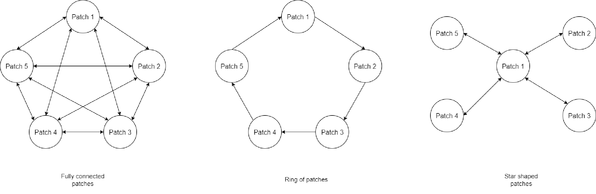
In this section, we simulate the model (2) to analyze different mobility patterns. Three different structures of the underlying network is considered, namely, fully connected network, ring of patches and a star like structure. Without loss of generality, we choose the number of patches to be five (see Fig. 2). The fixed parameters are taken from Table 1 and other parameters are $(\beta_{1},\beta_{2},\beta_{3},\beta_{4},\beta_{5})=(0.3,0.24,0.18,0.12,0.06)$ , $(\alpha_{1},\alpha_{2},\alpha_{3},\alpha_{4},\alpha_{5})=(0.4,0.35,0.3,0.25,0.2)$ and $\epsilon=0.005$ .

4.1.1 Scenario I: Fully connected patches

The dynamics of infected population in fully connected metapopulation structure is depicted in Fig. 3(A). The proposed model (2) is simulated with the fixed parameters. It can be observed that infected populations in patch 1 and patch 2 show similar trend of outbreak. However, patch 2 experiences a delayed outbreak as that of patch 1. As the epidemic is originated in patch 1, the subsequent patches have delayed outbreaks. It is also noted that the peak of the outbreaks are decreasing as the transmission rates vary in the same order.

4.1.2 Scenario II: Ring of patches

In this scenario, the underlying network is assumed to be a ring where migration occur in a cyclic pattern. We consider a confined case of system (2) by assuming that the patches are organized in a ring. Individuals in a given patch $i$ will only move to patch $i+1$ and from patch $n$ to patch $1$ , which is referred to as one-way migration. In this case all movement rates are zero except

\displaystyle m_{1n}>0,m_{21}>0,m_{32}>0,.......,m_{nn-1}>0.

Then the system (2) reduces to

$\displaystyle\displaystyle{\frac{dS_{i}}{dt}}$	$\displaystyle=$	$\displaystyle\Pi_{i}-\beta_{i}\frac{I_{i}}{N_{i}}S_{i}-\mu_{i}S_{i}-m_{i+1i}S_{i}+m_{ii-1}\Big(1-\frac{\alpha_{i-1}I_{i-1}}{N_{i-1}}\Big)S_{i-1},$
$\displaystyle\displaystyle{\frac{dE_{i}}{dt}}$	$\displaystyle=$	$\displaystyle\beta_{i}\frac{I_{i}}{N_{i}}S_{i}-(\gamma_{i}+\mu_{i})E_{i}-m_{i+1i}E_{i}+m_{ii-1}\frac{\alpha_{i-1}I_{i-1}}{N_{i-1}}S_{i-1}+(1-\xi_{i})m_{ii-1}E_{i-1},$	(4.1)
$\displaystyle\displaystyle{\frac{dI_{i}}{dt}}$	$\displaystyle=$	$\displaystyle\gamma_{i}E_{i}-(\sigma_{i}+\mu_{i}+\delta_{i})I_{i}-m_{i+1i}I_{i}+\xi_{i}m_{ii-1}E_{i-1}+(1-p_{i})m_{ii-1}I_{i-1},$
$\displaystyle\displaystyle{\frac{dR_{i}}{dt}}$	$\displaystyle=$	$\displaystyle\sigma_{i}I_{i}-\mu_{i}R_{i}-m_{i+1i}R_{i}+m_{ii-1}R_{i-1}+p_{i}m_{ii-1}I_{i-1},$

where

		$\displaystyle\text{if }i=1,\text{then }i-1=n$
		$\displaystyle\text{if }i=n,\text{then }i+1=1$

The time evolution of infected populations in this case are portrayed in Fig. 3(B). We observe that patch 1 undergoes recurrent epidemic i.e, multiple peaks are observed. Additionally, the magnitude of the peaks are higher than that of the fully connected case. The peaks for infected compartments of different patches are in decreasing order of magnitude as the transmission rates vary in the same order.

4.1.3 Scenario III: Star shaped patches

A star graph is a graph with one hub node in the center and remaining $n-1$ nodes connected to the center hub node. The number of connections or edges in a star graph of $n$ vertices is $n-1$ , where any node except the hub node has only one connection with the remaining nodes and the hub node has $n-1$ connections. Without loss of generality, we choose node $1$ as a hub node. In this case all movement rates are zero except

		$\displaystyle m_{1n}>0,m_{12}>0,m_{13}>0,.......,m_{1n-1}>0$
		$\displaystyle m_{n1}>0,m_{21}>0,m_{31}>0,.......,m_{n-11}>0$

Then the system (2) reduces to

$\displaystyle\displaystyle{\frac{dS_{1}}{dt}}$	$\displaystyle=$	$\displaystyle\Pi_{1}-\beta_{1}\frac{I_{1}}{N_{1}}S_{1}-\mu_{1}S_{1}-\sum_{j=1}^{n}m_{j1}S_{1}+\sum_{j=1}^{n}m_{1j}(1-\frac{\alpha_{j}I_{j}}{N_{j}})S_{j},$
$\displaystyle\displaystyle{\frac{dE_{1}}{dt}}$	$\displaystyle=$	$\displaystyle\beta_{1}\frac{I_{1}}{N_{1}}S_{1}-(\gamma_{1}+\mu_{1})E_{1}-\sum_{j=1}^{n}m_{j1}E_{1}+\sum_{j=1}^{n}m_{1j}\frac{\alpha_{j}I_{j}}{N_{j}}S_{j}+\sum_{j=1}^{n}(1-\xi_{1})m_{1j}E_{j},$
$\displaystyle\displaystyle{\frac{dI_{1}}{dt}}$	$\displaystyle=$	$\displaystyle\gamma_{1}E_{1}-(\sigma_{1}+\mu_{1}+\delta_{1})I_{1}-\sum_{j=1}^{n}m_{j1}I_{1}+\sum_{j=1}^{n}\xi_{1}m_{1j}E_{j}+\sum_{j=1}^{n}(1-p_{1})m_{1j}I_{j},$
$\displaystyle\displaystyle{\frac{dR_{1}}{dt}}$	$\displaystyle=$	$\displaystyle\sigma_{1}I_{1}-\mu_{1}R_{1}-\sum_{j=1}^{n}m_{j1}R_{1}+\sum_{j=1}^{n}m_{1j}R_{j}+\sum_{j=1}^{n}p_{1}m_{1j}I_{j},$	(4.2)
$\displaystyle\displaystyle{\frac{dS_{i}}{dt}}$	$\displaystyle=$	$\displaystyle\Pi_{i}-\beta_{i}\frac{I_{i}}{N_{i}}S_{i}-\mu_{i}S_{i}-m_{1i}S_{i}+m_{i1}\Big(1-\frac{\alpha_{1}I_{1}}{N_{1}}\Big)S_{1},$
$\displaystyle\displaystyle{\frac{dE_{i}}{dt}}$	$\displaystyle=$	$\displaystyle\beta_{i}\frac{I_{i}}{N_{i}}S_{i}-(\gamma_{i}+\mu_{i})E_{i}-m_{1i}E_{i}+m_{i1}\frac{\alpha_{1}I_{1}}{N_{1}}S_{1}+(1-\xi_{i})m_{i1}E_{1},$
$\displaystyle\displaystyle{\frac{dI_{i}}{dt}}$	$\displaystyle=$	$\displaystyle\gamma_{i}E_{i}-(\sigma_{i}+\mu_{i}+\delta_{i})I_{i}-m_{1i}I_{i}+\xi_{i}m_{i1}E_{1}+(1-p_{i})m_{i1}I_{1},$
$\displaystyle\displaystyle{\frac{dR_{i}}{dt}}$	$\displaystyle=$	$\displaystyle\sigma_{i}I_{i}-\mu_{i}R_{i}-m_{1i}R_{i}+m_{i1}R_{1}+p_{i}m_{i1}I_{1},$

where the first $4$ equation for $i=1$ and last $(4n-4)$ equations for $2\leq i\leq n$ .

The dynamics of infected population in star shaped patches is depicted in Fig. 3(C). In this case, the time series behave similarly as that of the fully connected case. However, the prevalence of infection in the patches 1 through 4 are different from the fully connected case.

Based on these observations, we can conclude that the underlying network structure is an important factor in metapopulation modelling. Different network topology may induce significant changes in the behavior of the epidemic disease. MATLAB codes to generate these time series are provided in GitHub ¹¹ 1 https://github.com/indrajitg-r/Metapop_IDT.

4.2 Effect of infection during travel

The proposed model (2) reduces to a model without infection during travel by putting $\alpha_{i}=0$ , $\xi_{i}=0$ and $p_{i}=0$ . Therefore, the system without infection during travel becomes

$\displaystyle\displaystyle{\frac{dS_{i}}{dt}}$	$\displaystyle=$	$\displaystyle\Pi_{i}-\beta_{i}\frac{I_{i}}{N_{i}}S_{i}-\mu_{i}S_{i}-\sum_{j=1}^{n}m_{ji}S_{i}+\sum_{j=1}^{n}m_{ij}S_{j},$
$\displaystyle\displaystyle{\frac{dE_{i}}{dt}}$	$\displaystyle=$	$\displaystyle\beta_{i}\frac{I_{i}}{N_{i}}S_{i}-(\gamma_{i}+\mu_{i})E_{i}-\sum_{j=1}^{n}m_{ji}E_{i}+\sum_{j=1}^{n}m_{ij}E_{j},$	(4.3)
$\displaystyle\displaystyle{\frac{dI_{i}}{dt}}$	$\displaystyle=$	$\displaystyle\gamma_{i}E_{i}-(\sigma_{i}+\mu_{i}+\delta_{i})I_{i}-\sum_{j=1}^{n}m_{ji}I_{i}+\sum_{j=1}^{n}m_{ij}I_{j},$
$\displaystyle\displaystyle{\frac{dR_{i}}{dt}}$	$\displaystyle=$	$\displaystyle\sigma_{i}I_{i}-\mu_{i}R_{i}-\sum_{j=1}^{n}m_{ji}R_{i}+\sum_{j=1}^{n}m_{ij}R_{j},$

The parameter values are same as previous section except $(\beta_{1},\beta_{2},\beta_{3},\beta_{4},\beta_{5})=\\ (0.14,0.12,0.1,0.08,0.06)$ , $(\alpha_{1},\alpha_{2},\alpha_{3},\alpha_{4},\alpha_{5})=(0.9,0.8,0.7,0.6,0.5)$ , and $\epsilon=0.3$ . Using this parameter set we simulate the models (2) to get the infected human population with infection during travel. On the other hand, (4.2) is simulated using this parameter set along with $\alpha_{i}=0$ , $\xi_{i}=0$ and $p_{i}=0$ to generate time series without infection during travel. The five infected compartments corresponding to five patches are reported in Fig. 4. From this figure, it can be observed that the endemic equilibrium is stable when there is infection during travel whereas the DFE is stable when there is no infection during travel. Therefore, it can be inferred that the infection during travel has the potential to alter stability of the system from disease-free to an endemic equilibrium. This reinforces that infection during travel may play a crucial role in disease transmission and persistence.

To investigate the effects of transmission coefficients during travel ( $\alpha_{i}$ ), we simulate the system (2) with variable $\alpha_{i}$ ’s ( $0.1\leq\alpha_{i}\leq 0.9$ ). The total number of infected people after 100 weeks is calculated for each cases. While varying $\alpha_{1}$ we keep other $\alpha_{i}$ ’s to be zero. This is done to distinguish individual effects of $\alpha_{i}$ ’s. The boxplots of infected population for $\alpha_{i}$ ’s are depicted in Fig. 5. All the coefficients show similar trends of total infected cases. However, the scales of total infection are slightly different for different $\alpha_{i}$ ’s. This also indicate that the transmission during transport has a significant role in disease transmission.

4.3 Effect of coupling strength and transmission coefficients

We draw contour plots of basic reproduction number ( $R_{0}$ ) with respect to the coupling strength ( $\epsilon$ ) and transmission coefficient during travel in patch 1 ( $\alpha_{1}$ ) to investigate their effects. The contour plot is depicted in left panel of Fig. 6. Nonlinear relations are observed for the variation in $\epsilon$ , initially $R_{0}$ increases with increase in $\epsilon$ and after a certain value is crossed the relation gets reversed. From this figure, it is also observed that $\epsilon$ has a dominant effect on $R_{0}$ over $\alpha_{1}$ . On the other hand, transmission coefficient in patch 1 ( $\beta_{1}$ ) has a positive impact on $R_{0}$ (see Fig. 6(B)). However, increasing $\epsilon$ shows a similar effect as that of Fig. 6(A).

Further, we examine contour plots of total infected people in all the five patches ( $\sum_{j=1}^{5}I_{i}(t)$ ) to clarify the effects of the parameters $\epsilon$ , $\alpha_{1}$ and $\beta_{1}$ . From Fig. 7, it can be observed that the total infection has nonlinear relationships with the transmission parameters $\alpha_{1}$ and $\beta_{1}$ and the coupling strength $\epsilon$ . However, for high values of coupling strength ( $\epsilon>0.25$ ), both the transmission coefficients have positive impact on the total infection. These contour plots reveal that the coupling strength is very crucial in disease spread and the impact may be counter-intuitive depending on situations.

4.4 Exit screening scenarios

Long distance passengers are checked for symptoms of an ongoing outbreak in a particular region. This checking or screening are necessary for respiratory disease outbreaks. Screening can be done before departure (exit screening) or after arrival (entry screening) to a certain place arino2016revisiting. For instance, WHO requested all SARS-CoV affected areas to screen departing passengers for SARS-CoV symptoms from March to May 2003 john2005border. Many Asian countries restarted these screenings during the 2009 pH1N1 spread. More recently, due to the high infectiousness of SARS-CoV-2 most of the countries have implemented exit screening as well as entry screening johansson2021reducing. Thermal scanners and test-kits have been used to screen the passengers for any symptoms. Here we consider imperfect border screening is implemented in all the patches with a certain level of efficiency. We assume that infectious patients are screened and restricted from travelling while other people are allowed to travel. We introduce a parameter $\kappa$ which measures the efficacy of exit screening. After incorporation of imperfect exit screening at a rate $\kappa$ , the model (2) become

$\displaystyle\displaystyle{\frac{dS_{i}}{dt}}$	$\displaystyle=$	$\displaystyle\Pi_{i}-\beta_{i}\frac{I_{i}}{N_{i}}S_{i}-\mu_{i}S_{i}-\sum_{j=1}^{n}m_{ji}S_{i}+\sum_{j=1}^{n}m_{ij}(1-\frac{\alpha_{j}I_{j}}{N_{j}})S_{j},$
$\displaystyle\displaystyle{\frac{dE_{i}}{dt}}$	$\displaystyle=$	$\displaystyle\beta_{i}\frac{I_{i}}{N_{i}}S_{i}-(\gamma_{i}+\mu_{i})E_{i}-\sum_{j=1}^{n}m_{ji}E_{i}+\sum_{j=1}^{n}m_{ij}\frac{\alpha_{j}I_{j}}{N_{j}}S_{j}+\sum_{j=1}^{n}(1-\xi_{i})m_{ij}E_{j},$	(4.4)
$\displaystyle\displaystyle{\frac{dI_{i}}{dt}}$	$\displaystyle=$	$\displaystyle\gamma_{i}E_{i}-(\sigma_{i}+\mu_{i}+\delta_{i})I_{i}-\kappa\sum_{j=1}^{n}m_{ji}I_{i}+\sum_{j=1}^{n}\xi_{i}m_{ij}E_{j}+\kappa\sum_{j=1}^{n}(1-p_{i})m_{ij}I_{j},$
$\displaystyle\displaystyle{\frac{dR_{i}}{dt}}$	$\displaystyle=$	$\displaystyle\sigma_{i}I_{i}-\mu_{i}R_{i}-\sum_{j=1}^{n}m_{ji}R_{i}+\sum_{j=1}^{n}m_{ij}R_{j}+\kappa\sum_{j=1}^{n}p_{i}m_{ij}I_{j},$

The time evolution of the infected compartments of different patches are depicted in Fig. 8. The screening efficacy $\kappa$ is taken to be $\kappa=1$ for no screening and decreasing values of $\kappa$ indicate increasing screening efficacy. All the panels in Fig. 8 show similar trends of decrease in infection prevalence. However, since the infection prevalence is higher in patch 1, exit screening will have negligible effect in the prevalence. To quantify the effects of different exit screening levels, we now calculate the percentage reduction in the infection during 1000 days from infection onset. The percentage reduction is computed using the following basic formula

\displaystyle\textmd{Percentage reduction in infected persons}=\frac{\textmd{Base value of infected persons}-\textmd{Model output}}{\textmd{Base value of infected persons}}\times 100.

The percentage reductions are reported in Table 2. It can be observed that the infection in the patch 1 will increase for different exit screening scenarios. However, all the other patches show significant decrease in cases. This indicate that in a metapopulation, the patch with high prevalence and high transmission rate will not benefit from the exit screening. But, the collectively it can be inferred that the infection will show decreasing trends if exit screening is implemented.

Table 2: Percentage reduction in infectious people for different exit screening scenarios.

Parameter	Values	$I_{1}(t)$	$I_{2}(t)$	$I_{3}(t)$	$I_{4}(t)$	$I_{5}(t)$
$\kappa$	0.75	-1.13	6.22	9.50	9.55	10.05
	0.5	-2.30	13.03	19.27	20.09	20.29
	0.25	-3.45	20.59	29.37	30.50	30.77

4.5 Emergence of a new strain

In this subsection, we numerically study the effect of a new strain of the virus on the overall population dynamics. Respiratory disease causing viruses such as influenza, SARS-CoV, MERS-CoV, SARS-CoV-2 etc are mostly RNA viruses and are prone to mutations lyons2018mutation; garcia2021multiple. Therefore, it is important to investigate multi-strain dynamics of the metapopulation. We consider a simple two strain model for the propagation of the virus (see Fig. 9) in each patch khyar2020global.

We assume that the patches are connected through migration and the transmission of both the strains are possible during travel. Further, the transmission rates for both the strains of the virus are taken to be different whereas all other parameters are taken to be same. Thus, taking these assumptions into consideration, the system (2) becomes the following system of equations

$\displaystyle\displaystyle{\frac{dS_{i}}{dt}}$	$\displaystyle=$	$\displaystyle\Pi_{i}-\frac{\beta^{1}_{i}I^{1}_{i}+\beta^{2}_{i}I^{2}_{i}}{N_{i}}S_{i}-\mu_{i}S_{i}-\sum_{j=1}^{n}m_{ji}S_{i}+\sum_{j=1}^{n}m_{ij}(1-\frac{\alpha^{1}_{j}I^{1}_{j}+\alpha^{2}_{j}I^{2}_{j}}{N_{j}})S_{j},$
$\displaystyle\displaystyle{\frac{dE^{1}_{i}}{dt}}$	$\displaystyle=$	$\displaystyle\beta^{1}_{i}\frac{I^{1}_{i}}{N_{i}}S_{i}-(\gamma_{i}+\mu_{i})E^{1}_{i}-\sum_{j=1}^{n}m_{ji}E^{1}_{i}+\sum_{j=1}^{n}m_{ij}\frac{\alpha^{1}_{j}I^{1}_{j}}{N_{j}}S_{j}+\sum_{j=1}^{n}(1-\xi_{i})m_{ij}E^{1}_{j},$
$\displaystyle\displaystyle{\frac{dE^{2}_{i}}{dt}}$	$\displaystyle=$	$\displaystyle\beta^{2}_{i}\frac{I^{2}_{i}}{N_{i}}S_{i}-(\gamma_{i}+\mu_{i})E^{2}_{i}-\sum_{j=1}^{n}m_{ji}E^{2}_{i}+\sum_{j=1}^{n}m_{ij}\frac{\alpha^{2}_{j}I^{2}_{j}}{N_{j}}S_{j}+\sum_{j=1}^{n}(1-\xi_{i})m_{ij}E^{2}_{j},$	(4.5)
$\displaystyle\displaystyle{\frac{dI^{1}_{i}}{dt}}$	$\displaystyle=$	$\displaystyle\gamma_{i}E^{1}_{i}-(\sigma_{i}+\mu_{i}+\delta_{i})I^{1}_{i}-\sum_{j=1}^{n}m_{ji}I^{1}_{i}+\sum_{j=1}^{n}\xi_{i}m_{ij}E^{1}_{j}+\sum_{j=1}^{n}(1-p_{i})m_{ij}I^{1}_{j},$
$\displaystyle\displaystyle{\frac{dI^{2}_{i}}{dt}}$	$\displaystyle=$	$\displaystyle\gamma_{i}E^{2}_{i}-(\sigma_{i}+\mu_{i}+\delta_{i})I^{2}_{i}-\sum_{j=1}^{n}m_{ji}I^{2}_{i}+\sum_{j=1}^{n}\xi_{i}m_{ij}E^{2}_{j}+\sum_{j=1}^{n}(1-p_{i})m_{ij}I^{2}_{j},$
$\displaystyle\displaystyle{\frac{dR_{i}}{dt}}$	$\displaystyle=$	$\displaystyle\sigma_{i}(I^{1}_{i}+I^{2}_{i})-\mu_{i}R_{i}-\sum_{j=1}^{n}m_{ji}R_{i}+\sum_{j=1}^{n}m_{ij}R_{j}+\sum_{j=1}^{n}p_{i}m_{ij}(I^{1}_{j}+I^{2}_{j}),$

The model (4.5) is simulated using parameter values from Table 1 and other parameters are taken as $\epsilon=0.01$ $(\alpha^{1}_{1},\alpha^{1}_{2},\alpha^{1}_{3},\alpha^{1}_{4},\alpha^{1}_{5})=(0.16,0.14,0.12,0.1,0.08)$ , $(\alpha^{2}_{1},\alpha^{2}_{2},\alpha^{2}_{3},\alpha^{2}_{4},\alpha^{2}_{5})=(0.2,0.2,0.2,0.2,0.2)$ , $d_{12}=d_{21}=100$ , $d_{13}=d_{31}=110$ , $d_{14}=d_{41}=120$ , $d_{15}=d_{51}=130$ , $d_{23}=d_{32}=140$ , $d_{24}=d_{42}=150$ , $d_{25}=d_{52}=160$ , $d_{34}=d_{43}=170$ , $d_{35}=d_{53}=180$ , $d_{45}=d_{54}=190$ and $(\nu_{1},\nu_{2},\nu_{3},\nu_{4},\nu_{5})=(7,6,5,4,3)$ . $\beta^{1}_{i}$ and $\beta^{2}_{i}$ are varied in the range $(0.1,0.4)$ . Initially, we examine the time evolution of both the strains. To this end, we simulate the model (2) with different transmission rates and initial conditions $(S_{1}(0),E_{1}(0),I_{1}(0),R_{1}(0))=(100000,100,10,0)$ and $(S_{i}(0),E_{i}(0),I_{i}(0),R_{i}(0))=(100000,0,0,0)$ for i=2,3,4,5. After 200 days, a second strain is seeded in patch 3. To do this numerically, we take the end points of the state variables from the 200^th day and plug in them to the system (4.5) along with the number of strain 2 infected in patch 3 is 1. However, the initial strain 2 infected persons ( $I^{2}_{i}$ , i=2,3,4,5) in other patches and strain 2 exposed persons ( $E^{2}_{i}$ , i=1,2,3,4,5) in all patches are taken to be zero. Depending on the transmission coefficients $\beta^{1}_{i}$ and $\beta^{2}_{i}$ , we observe that either the first strain infected persons persist (see Fig. 10) or the second strain infected persons persist (see Fig. 11).

It can be observed that the two co-circulating strains will not co-exist in the community in a long run. This effect is know as competitive exclusion principle in mathematical epidemiology martcheva2015introduction. Fig. 11 depicts the persistence of second strain infection and extinction of strain 1 infection in patch 1 and patch 5. It can be observed that both the strains co-exist for a very short period. However, a transition is observed for both the patches i.e, infected persons with strain 1 go to extinction after emergence of the strain 2 infection. Additionally, it is seen that strain 1 infection may have persisted if second strain was not introduced in the population.

Further, to investigate the behavior of the equilibrium value of the second strain with respect to the transmission coefficient $\beta^{2}_{i}$ , we draw the bifurcation diagrams 12. It can be observed that the equilibrium value remains at zero until $\beta^{2}_{i}$ cross a certain threshold. This gives rise to a forward transcritical bifurcation. This indicate that the strain 2 free equilibrium and strain 2 endemic equilibrium will change stability after a certain threshold value of $\beta^{2}_{i}$ .

5 Discussion

In this paper, we propose and analyze a novel metapopulation model with infection during transport. We extend a two-patch SIS model of Arino et. al arino2016revisiting to incorporate recovery and incubation during transport. We also consider the migration terms to be related to distance between patches and perceived severity of the disease. The general n-patch model is analyzed mathematically. Positivity and boundedness of the proposed model are established and an invariant region for the system is obtained. Existence of the unique disease-free equilibrium has been proved and the local stability of this equilibrium is governed by the basic reproduction number ( $R_{0}$ ). Moreover, if the movement matrices satisfy certain conditions and $R_{0}<1$ , then the DFE is globally asymptotically stable. Existence of an endemic equilibrium is also established under some conditions.

Extensive numerical experiments using different parameter sets are performed to get insight into the transmission process. Different migration matrices are considered to study the network topology such as fully connected, ring of patches or star-like network (as depicted in Fig. 2). Keeping all the parameters fixed except the migration matrix, we simulate the system which reveal that different network topology does have a effect on the prevalence of the disease in different patches (see Fig. 3). Further numerical simulations suggest that infection during travel has the potential to move the equilibrium from disease free to an endemic state (see Fig. 4). The transmission rates during travel ( $\alpha_{i}$ ) are then varied individually to quantify their effects on disease prevalence. It is observed that all the $\alpha_{i}$ ’s play significant role in disease transmission (see Fig. 5). Furthermore, numerically we observe that depending on the value of coupling strength, transmission coefficients ( $\beta_{1}$ and $\alpha_{1}$ ) may show nonlinear effects on $R_{0}$ and total number of infectives. The coupling strength also show some nonlinear relationships with both $R_{0}$ and total number of infectious persons (as seen in Fig. 6 and Fig. 7). Epidemiologically, this indicate that while dealing real epidemic curves, modellers have to be very careful about the choice of coupling strengths. Modelling diseases in a metapopulation setting is inherently related to the migration rates between patches. From control strategic point of view, restricting migration of infectives between patches are studied for disease suppression. Thus, various exit screening scenarios were studied to get a better understanding of the system. We observe that implementation of imperfect exit screening in all the patches may have negative impact on the patch with high prevalence and high transmission rate (patch 1 in this case). However, all other patches experience significant reduction in infectious persons. Finally, we studied the emergence of a new variant strain of the virus and its effect on the dynamics of the previous strain. It is observed that first strain is persistent or the second strain is persistent in the long run depending on the transmission coefficients. However, two strain will not co-exist in the population at equilibrium. The equilibrium values of the second strain also show threshold-like behaviour with respect to the transmission coefficients of the second strain. This indicate that transmission rates are very crucial for the persistence or extinction of the new strain in the community.

Acknowledgements

Research of IG is supported by National Board for Higher Mathematics (NBHM) postdoctoral fellowship (Ref. No: 0204/3/2020/R & D-II/2458). SSN receives senior research fellowship from CSIR, Government of India, New Delhi. The work of SR is partially supported by SERB MATRICS grants MTR/2020/000186 and MSC/2020/00028 of the Government of India.

References

[1] Julien Arino. Spatio-temporal spread of infectious pathogens of humans. Infectious Disease Modelling, 2(2):218–228, 2017.
[2] Julien Arino, Chengjun Sun, and Wei Yang. Revisiting a two-patch SIS model with infection during transport. Mathematical Medicine and Biology: A Journal of the IMA, 33(1):29–55, 2016.
[3] Justin Bahl, Martha I Nelson, Kwok H Chan, Rubing Chen, Dhanasekaran Vijaykrishna, Rebecca A Halpin, Timothy B Stockwell, Xudong Lin, David E Wentworth, Elodie Ghedin, et al. Temporally structured metapopulation dynamics and persistence of influenza a h3n2 virus in humans. Proceedings of the National Academy of Sciences, 108(48):19359–19364, 2011.
[4] Abraham Berman and Robert J Plemmons. Nonnegative matrices in the mathematical sciences. SIAM, 1994.
[5] Nam Parshad Bhatia and Giorgio P Szegö. Stability theory of dynamical systems. Springer Science & Business Media, 2002.
[6] Ben M Bolker and Bryan Thomas Grenfell. Chaos and biological complexity in measles dynamics. Proceedings of the Royal Society of London. Series B: Biological Sciences, 251(1330):75–81, 1993.
[7] Gabrielle Brankston, Leah Gitterman, Zahir Hirji, Camille Lemieux, and Michael Gardam. Transmission of influenza a in human beings. The Lancet infectious diseases, 7(4):257–265, 2007.
[8] Fred Brauer and Pauline van den Driessche. Models for transmission of disease with immigration of infectives. Mathematical Biosciences, 171(2):143–154, 2001.
[9] Marisa C Eisenberg, Zhisheng Shuai, Joseph H Tien, and P Van den Driessche. A cholera model in a patchy environment with water and human movement. Mathematical Biosciences, 246(1):105–112, 2013.
[10] Fatima Etbaigha, Allan R. Willms, and Zvonimir Poljak. An seir model of influenza a virus infection and reinfection within a farrow-to-finish swine farm. PLoS One, 13(9):e0202493, 2018.
[11] Hiroyuki Furuya. Risk of transmission of airborne infection during train commute based on mathematical model. Environmental health and preventive medicine, 12(2):78–83, 2007.
[12] Wilfredo F Garcia-Beltran, Evan C Lam, Kerri St Denis, Adam D Nitido, Zeidy H Garcia, Blake M Hauser, Jared Feldman, Maia N Pavlovic, David J Gregory, Mark C Poznansky, et al. Multiple sars-cov-2 variants escape neutralization by vaccine-induced humoral immunity. Cell, 184(9):2372–2383, 2021.
[13] HONGBIN Guo and MICHAEL Y Li. Global stability of the endemic equilibrium of a tuberculosis model with immigration and treatment. Canad. Appl. Math. Quart, 19:1–18, 2011.
[14] Ying-Hen Hsieh, P Van den Driessche, and Lin Wang. Impact of travel between patches for spatial spread of disease. Bulletin of mathematical biology, 69(4):1355–1375, 2007.
[15] Michael A Johansson, Hannah Wolford, Prabasaj Paul, Pamela S Diaz, Tai-Ho Chen, Clive M Brown, Martin S Cetron, and Francisco Alvarado-Ramy. Reducing travel-related sars-cov-2 transmission with layered mitigation measures: symptom monitoring, quarantine, and testing. BMC medicine, 19(1):1–13, 2021.
[16] Ronald K St John, Arlene King, Dick De Jong, Margaret Bodie-Collins, Susan G Squires, and Theresa WS Tam. Border screening for sars. Emerging infectious diseases, 11(1):6, 2005.
[17] Charles R Johnson and Roger A Horn. Matrix analysis. Cambridge university press Cambridge, 1985.
[18] Omar Khyar and Karam Allali. Global dynamics of a multi-strain seir epidemic model with general incidence rates: application to covid-19 pandemic. Nonlinear Dynamics, 102(1):489–509, 2020.
[19] Luke D Knibbs, Lidia Morawska, and Scott C Bell. The risk of airborne influenza transmission in passenger cars. Epidemiology & Infection, 140(3):474–478, 2012.
[20] Diána Knipl. Stability criteria for a multi-city epidemic model with travel delays and infection during travel. Electronic Journal of Qualitative Theory of Differential Equations, 2016:1–22, 2016.
[21] Joseph P La Salle. The stability of dynamical systems. SIAM, 1976.
[22] Michael Y Li, John R Graef, Liancheng Wang, and János Karsai. Global dynamics of a seir model with varying total population size. Mathematical biosciences, 160(2):191–213, 1999.
[23] Junli Liu, Jianhong Wu, and Yicang Zhou. Modeling disease spread via transport-related infection by a delay differential equation. The Rocky Mountain Journal of Mathematics, pages 1525–1540, 2008.
[24] Luju Liu, Xiao-Qiang Zhao, and Yicang Zhou. A tuberculosis model with seasonality. Bulletin of Mathematical Biology, 72(4):931–952, 2010.
[25] Alun L Lloyd and Vincent AA Jansen. Spatiotemporal dynamics of epidemics: synchrony in metapopulation models. Mathematical biosciences, 188(1-2):1–16, 2004.
[26] Daniel M Lyons and Adam S Lauring. Mutation and epistasis in influenza virus evolution. Viruses, 10(8):407, 2018.
[27] P. van den Driessche Mahin Salmani. A model for disease transmission in a patchy environment. Discrete & Continuous Dynamical Systems - B, 6(1):185–202, 2006.
[28] Alexandra Mangili and Mark A Gendreau. Transmission of infectious diseases during commercial air travel. The Lancet, 365(9463):989–996, 2005.
[29] Maia Martcheva. An introduction to mathematical epidemiology, volume 61. Springer, 2015.
[30] Yukihiko Nakata. On the global stability of a delayed epidemic model with transport-related infection. Nonlinear Analysis: Real World Applications, 12(6):3028–3034, 2011.
[31] Abhishek Senapati, Tridip Sardar, and Joydev Chattopadhyay. A cholera metapopulation model interlinking migration with intervention strategies—a case study of zimbabwe (2008–2009). Journal of Biological Systems, 27(02):185–223, 2019.
[32] Hal L Smith and Paul Waltman. The theory of the chemostat: dynamics of microbial competition, volume 13. Cambridge university press, 1995.
[33] Chengjun Sun, Wei Yang, Julien Arino, and Kamran Khan. Effect of media-induced social distancing on disease transmission in a two patch setting. Mathematical biosciences, 230(2):87–95, 2011.
[34] Yasuhiro Takeuchi, Xianning Liu, and Jingan Cui. Global dynamics of SIS models with transport-related infection. Journal of mathematical analysis and applications, 329(2):1460–1471, 2007.
[35] Yasuhiro Takeuchi, Yasuhisa Saito, et al. Spreading disease with transport-related infection. Journal of theoretical biology, 239(3):376–390, 2006.
[36] Pauline Van den Driessche and James Watmough. Reproduction numbers and sub-threshold endemic equilibria for compartmental models of disease transmission. Mathematical biosciences, 180(1-2):29–48, 2002.
[37] Joseph T Wu, Kathy Leung, and Gabriel M Leung. Nowcasting and forecasting the potential domestic and international spread of the 2019-ncov outbreak originating in wuhan, china: a modelling study. The Lancet, 395(10225):689–697, 2020.

Metapopulation dynamics of a respiratory disease with infection during travel

Abstract

Keywords:

1 Introduction

2 Model description

3 Mathematical analysis

3.1 Positivity and boundedness of the solution

Proposition 3.1.

Proof.

Proposition 3.2.

Proof.

Corollary 3.1.

3.2 Stability of disease-free equilibrium and basic reproduction number

Theorem 3.1.

3.2.1 Basic Reproduction Number

3.2.2 Bounds on R0R_{0}

Theorem 3.2.

Proof.

3.2.3 Global stability of disease-free equilibrium

Theorem 3.3.

Proof.

4 Numerical simulations

4.1 Effect of network topology

4.1.1 Scenario I: Fully connected patches

4.1.2 Scenario II: Ring of patches

4.1.3 Scenario III: Star shaped patches

4.2 Effect of infection during travel

4.3 Effect of coupling strength and transmission coefficients

4.4 Exit screening scenarios

4.5 Emergence of a new strain

5 Discussion

Acknowledgements

References

3.2.2 Bounds on $R_{0}$