Chordal and factor-width decompositions for scalable semidefinite
and polynomial optimizationJournal: Annual Reviews in Control
Abstract
Chordal and factor-width decomposition methods for semidefinite programming and polynomial optimization have recently enabled the analysis and control of large-scale linear systems and medium-scale nonlinear systems. Chordal decomposition exploits the sparsity of semidefinite matrices in a semidefinite program (SDP), in order to formulate an equivalent SDP with smaller semidefinite constraints that can be solved more efficiently. Factor-width decompositions, instead, relax or strengthen SDPs with dense semidefinite matrices into more tractable problems, trading feasibility or optimality for lower computational complexity. This article reviews recent advances in large-scale semidefinite and polynomial optimization enabled by these two types of decomposition, highlighting connections and differences between them. We also demonstrate that chordal and factor-width decompositions allow for significant computational savings on a range of classical problems from control theory, and on more recent problems from machine learning. Finally, we outline possible directions for future research that have the potential to facilitate the efficient optimization-based study of increasingly complex large-scale dynamical systems.
Keywords:
Chordal sparsity, semidefinite optimization, polynomial optimization, sum-of-squares, matrix decomposition, factor-width decomposition, large-scale systems, scalability1 Introduction
The design of innovative technology capable to address the challenges of the 21st century relies on the ability to analyze, predict, and control large-scale complex systems, which are typically nonlinear and may interact over networks (Murray et al. 2003; Astrom & Kumar 2014). Convex optimization is one of the key tools for achieving these goals, because many questions related to the stability and operational safety of dynamical systems, the synthesis of optimal control policies, and the certification of robust performance can be posed as (or relaxed into) convex optimization problems. Very often, these take the form of semidefinite programs (SDPs)—linear optimization problems with positive semidefinite matrix variables.
For linear systems, well-known methods based on linear matrix inequalities (LMIs) enable one to tackle a wide range of problems, including the study of stability, reachability, input-to-state and input-to-output properties, and the design of optimal and robust control strategies (Boyd et al. 1994; Zhou et al. 1996; Kailath 1980). Methods based on LMIs have been successfully applied across a broad spectrum of applications, including automotive applications (Rajamani 2011), flight control (Giulietti et al. 2000), power grids (Riverso et al. 2014; Sadabadi et al. 2016), and traffic systems (Ploeg et al. 2013; Li et al. 2017; Zheng et al. 2020). For nonlinear systems with polynomial dynamics, SDP relaxations based on sum-of-squares polynomials (or, equivalently, moment sequences) enable stability analysis (Parrilo 2000; Anderson & Papachristodoulou 2015; Peet & Papachristodoulou 2012; Henrion & Garulli 2005), the estimation of regions of attractions (Valmorbida & Anderson 2017; Korda et al. 2013; Topcu et al. 2009; Henrion & Korda 2014; Chesi 2011) and reachable sets (Jones & Peet 2019; Magron et al. 2019), safety verification (Prajna et al. 2007; Miller et al. 2021), analysis of extreme or average behaviour (Fantuzzi et al. 2016; Fantuzzi & Goluskin 2020; Korda et al. 2021; Kuntz et al. 2016; Goluskin 2020), and optimal control (Prajna et al. 2004; Henrion & Lasserre 2006; Lasserre et al. 2008; Han & Tedrake 2018; Majumdar et al. 2014; Lasagna et al. 2016).
A widespread view since the 1990s is that, once a control problem is reformulated as an SDP or relaxed into one, then the problem is effectively solved (Parrilo & Lall 2003; Boyd et al. 1994). In today’s world of large-scale, complex systems, however, this is no longer true, and the formulation of SDPs that can be solved in practice requires further thought. This is because, even though SDPs can theoretically be solved using algorithms with polynomial-time complexity (Vandenberghe & Boyd 1996; Ye 2011; Nesterov & Nemirovski 1994; Nesterov 2003; Nemirovski 2006), the very-large-scale SDPs encountered in real-life applications require prohibitively large computational resources in practice. One particular bottleneck is the complexity of handling large semidefinite constraints; for instance, each iteration of classical interior-point algorithms requires time and memory (Nesterov 2003, Section 4.3.3), where is the size of semidefinite constraint and is the number of equality constraints. The majority of established general-purpose SDP solvers currently available, therefore, cannot handle large problems (e.g., with larger than a few hundreds and larger than a few thousands) on a regular computer. Consequently, the application of SDP-based frameworks for analysis and control is currently limited to medium-scale linear systems and small-scale nonlinear ones.
Overcoming these scalability issues is a problem that has received much attention in recent years (Majumdar et al. 2020; De Klerk 2010; Vandenberghe et al. 2015; Ahmadi et al. 2017b), and significant progress has been made through a number of different approaches. Most of them are related by a simple, yet powerful, underlying idea: decompose a large positive semidefinite matrix as a sum of structured ones, for which it is easier to impose positivity.
One type of structured decomposition considers sums of low-rank matrices (Burer et al. 2002; Burer & Monteiro 2003; Burer & Monteiro 2005; Burer & Choi 2006). Specifically, one writes for some vectors , where is a parameter to be chosen, and optimizes over the choice of such vectors. Such a decomposition is guaranteed to exist for a properly chosen , and there are explicit lower bounds on this parameter ensuring that the global minimum of the decomposed problem coincides with that of the original SDP (Pataki 1998). However, while low-rank decomposition can bring considerable performance gains on large SDPs, it transforms a convex problem into a nonconvex one. Solution algorithms for the latter cannot be guaranteed to converge to the global minimum unless the original SDP is sufficiently “smooth” and is large enough (Waldspurger & Waters 2020; Boumal et al. 2020).
A second type of structured decomposition, which we focus on in this paper, considers sums of sparse matrices. In this case, one writes for positive semidefinite matrices that are nonzero only on a certain (and, ideally, small) principal submatrix. The choice of these principal submatrices is crucial in determining the particular type of matrix decomposition, as well as its properties. Two common selection strategies distinguish whether the original matrix is dense or sparse.
If is sparse, the principal submatrices are usually indexed by the maximal cliques of the sparsity graph of ; these notions will be defined precisely in Section 2, but are illustrated in Figure 1.1. When the sparsity graph is chordal, meaning that all cycles of length larger than three have an edge between nonconsecutive vertices, the existence of a clique-based decomposition is guaranteed (Agler et al. 1988; Kakimura 2010; Griewank & Toint 1984). One can therefore replace the optimization of the large matrix with the optimization of the matrices without any loss of generality. Together with a dual result on the existence of positive semidefinite matrix completions (Grone et al. 1984), this chordal decomposition strategy enables one to significantly reduce the computational complexity of SDPs involving sparse positive semidefinite matrices (Fukuda et al. 2001; Nakata et al. 2003; Kim et al. 2011; Vandenberghe et al. 2015).
When is dense, instead, each matrix in the decomposition is chosen to be nonzero only on one of the possible principal submatrices of , where the parameter is specified a priori. This type of decomposition leads to factor-width- inner approximations of the positive semidefinite cone (Boman et al. 2005), which are conservative but improve as is increased. When , optimizing over the matrices , rather than over the original dense matrix , leads to SDPs with small positive semidefinite cones, which can often be handled efficiently. In the extreme case , one obtains a second-order cone program, for which scalable algorithms exist (Alizadeh & Goldfarb 2003).
This paper offers a comprehensive review of chordal and factor-width- decomposition methods, as well as of their application to large-scale semidefinite programming and polynomial optimization. Our goal is to introduce practitioners in control theory to the latest advances in these fields, which over the last decade or so have increased the scale of systems for which optimization-based frameworks for analysis and control can be implemented at a reasonable cost. Examples of problems that can now be handled efficiently include the analysis and synthesis of large-scale linear networked systems (Mason & Papachristodoulou 2014; Zheng et al. 2018c; Zheng et al. 2018d; Andersen et al. 2014b), the stability analysis and the approximation of regions of attraction for sparse nonlinear systems (Schlosser & Korda 2020; Tacchi et al. 2019a; Zheng et al. 2019a; Ahmadi & Majumdar 2019), optimal power flow in power grids (Andersen et al. 2014a; Jabr 2011; Molzahn et al. 2013), and numerous problems in machine learning (Batten et al. 2021; Newton & Papachristodoulou 2021; Kim et al. 2009; Dahl et al. 2008; Zhang et al. 2018; Latorre et al. 2020; Chen et al. 2020b). We hope that knowledge of the advanced optimization techniques discussed here can assist control theorists in developing efficient modelling frameworks that can be applied much more widely and, crucially, to increasingly complex large-scale systems.
1.1 Outline
After introducing relevant graph-theoretic notions in section 2, we discuss chordal decomposition methods for general SDPs in section 3. Section 4 looks at decomposition methods for sparse polynomial optimization problems, which arise when relaxing analysis and control problems for nonlinear systems. Factor-width- decompositions for dense matrices are discussed in section 5. Section 6 presents examples of how matrix decomposition can be applied to some classical control problems and to some recent problems in machine learning. Section 7 draws conclusions and outlines possible directions for future research.
1.2 Basic notation
Mathematical symbols are defined as necessary in each of the following sections, but we summarize common notation here. The -dimensional Euclidean space, the vector space of real symmetric matrices, and the cone of positive semidefinite symmetric matrices are denoted, respectively, by , , and . Angled brackets are used to denote the inner product in any of these spaces; in particular, when and when . We often write instead of when the matrix size is clear from the context or is unimportant, and write if is strictly positive definite.
2 Chordal graphs and matrix decomposition
This section reviews chordal graphs and their applications to sparse matrix decomposition. Matrix decomposition is central to many sparsity-exploiting techniques for semidefinite and polynomial optimization. Detailed introductions to chordal graphs can be found in the surveys by Blair & Peyton 1993 and Rose 1970, and in the monographs by Vandenberghe et al. 2015 and Golumbic 2004. We first introduce some graph-theoretic notions in Section 2.1, and then given an overview of classical matrix decomposition and completion results in Section 2.2. Extensions to sparse block-partitioned matrices are discussed in Section 2.3.
2.1 Chordal graphs
A graph is defined by a set of vertices and a set of edges . A graph is undirected if implies that . A path in is a sequence of edges that connect a sequence of distinct vertices. A graph is connected if there is a path between any two vertices, and complete if any two vertices are connected by an edge, i.e., . The subgraph induced by a subset of vertices is the undirected graph with vertices and edges . A subset of vertices is called a clique if the subgraph induced by is complete. If is not contained in any other clique, it is a maximal clique. The number of vertices in is denoted by .
A cycle of length in a graph is a set of pairwise distinct vertices such that and for . A chord in a cycle is an edge connecting two nonconsecutive vertices.
Definition 2.1.
An undirected graph is chordal if every cycle of length has at least one chord.
Examples of chordal graphs are given in fig. 2.1. Observe also that many common types of graphs are chordal, including chains, acyclic undirected graphs (i.e., graphs with no cycles, such as trees), undirected graphs with cycles of length no greater than three, and complete graphs.


Chordal graphs have a number of properties that make them easy to handle computationally. For example, a connected chordal graph has at most maximal cliques, and they can be identified in linear time with respect to the number of vertices and edges (Vandenberghe et al. 2015) using, for instance, Algorithm 2 in Appendix C. In addition, any induced subgraph of a chordal graph is chordal because cycles in the subgraph are also cycles in the original graph. This is a useful fact in several induction proofs using chordality in Blair & Peyton 1993. Finally, chordal graphs admit a so-called perfect elimination ordering of the vertices, which is central to the zero fill-in property of Cholesky factorizations for sparse matrices. These two properties are reviewed in Appendix A.
Given the rich structure implied by chordality, it is very often convenient to extend a nonchordal graph into a chordal graph with larger edge set , which is called a chordal extension of . Usually, a graph admits many different chordal extensions, including the trivial one with edge set obtained by completion, and the one obtained by completing only the graph’s connected components. Finding a minimal chordal extension, meaning that the smallest possible number of additional edges has been added, is an NP-complete problem (Yannakakis 1981). However, approximately minimal chordal extensions can often be constructed in practice using heuristic strategies such as the maximum cardinality search (Berry et al. 2004) and the symbolic Cholesky factorization with approximately minimum degree ordering (Fukuda et al. 2001; Vandenberghe et al. 2015).
fig. 2.2 illustrates these concepts. The graph in fig. 2.2(a) is not chordal, but can be extended to the chordal graph in fig. 2.2(b) by adding edge , edge , or both. The first two extensions are minimal, while the latter is the trivial extension by completion. The minimal chordal extension obtained by adding edge has two maximal cliques, and .
2.2 Sparse matrix decomposition
This subsection reviews two fundamental results on the decomposition of sparse positive semidefinite matrices whose sparsity can be described using chordal graphs.
2.2.1 Sparse symmetric matrices
Fix any positive integer and set . Given an undirected graph , we say that a symmetric matrix has a sparsity graph (alternatively, sparsity pattern ) if when . We denote the space of sparse symmetric matrices by
For example, the graph11 1 Throughout, we assume that each vertex has a self-loop, unless otherwise noted. We omit the self-loops when plotting a graph. in fig. 2.2(b) describes the sparsity pattern of the matrix
| (2.1) |
where each entry may be nonzero or zero. Similarly, the symbolic matrices in fig. 2.3 have sparsity patterns described by the graphs in fig. 2.1.
Given , the diagonal elements and the off-diagonal elements with may be nonzero or zero. Thus, if and is an extension of the edge set, then we also have . In this paper, we are especially interested in chordal extensions of sparsity pattern. For simplicity, we will say that a matrix has a chordal sparsity pattern if its corresponding sparsity graph is chordal. Of course, this can always be achieved via chordal extension.
In what follows, it will be convenient to refer to particular principal submatrices of a sparse matrix, indexed by the maximal cliques of its sparsity graph. Given a clique of , we define a matrix with entries
| (2.2) |
where is the -th vertex22 2 The elements of can be sorted in any convenient order. We implicitly use the natural ordering in this work, but using a different one simply amounts to a permutation of the columns of . Given , the definition of implies that the operation extracts the principal submatrix of indexed by the clique . Conversely, the operation “inflates” a matrix into a sparse symmetric matrix that has as its principal submatrix indexed by , and is zero otherwise. For example, the chordal graph in fig. 2.2(b) has a maximal clique , and the corresponding matrix is
For the sparse matrix in eq. 2.1 and any matrix , we have
2.2.2 Cone of sparse positive semidefinite matrices
Denote the set of positive semidefinite matrices with sparsity pattern by
This set is a convex cone because it is the intersection of a subspace and a convex cone. If is a chordal graph, can be represented using smaller but coupled convex cones, as stated in the following result (Agler et al. 1988; Griewank & Toint 1984; Kakimura 2010).
Theorem 2.1.
Let be a chordal graph with maximal cliques . Then, if and only if there exist matrices for such that
| (2.3) |
The “if” part of theorem 2.1 is immediate, since a sum of positive semidefinite matrices is positive semidefinite. The “only if” part, instead, can be proven using the zero fill-in property of sparse Cholesky factorization for (Vandenberghe et al. 2015, Section 9.2); see appendices A and B for details. A similar elementary proof given by Kakimura 2010, based on simple linear algebra and perfect elimination orderings for chordal graphs, reveals that one can impose a rank constraint in the decomposition eq. 2.3: there exist with such that eq. 2.3 holds.
Remark 2.1.
The chordality assumption in theorem 2.1 is necessary. For every nonchordal pattern , while particular matrices in admit the decomposition eq. 2.3, there always exist matrices in that do not; see Vandenberghe et al. 2015 for an explicit example. In addition, the decomposition eq. 2.3 generally requires all maximal cliques , even when a subset of maximal cliques has already covered the sparsity pattern (that is with ). An example of this is given in Appendix C.
Example 2.1.
Consider the positive semidefinite matrix
| (2.4) |
whose sparsity graph is a chordal chain graph with three vertices, edge set , and maximal cliques and . Theorem 2.1 guarantees that the decomposition eq. 2.3 exists. Indeed, we have
and
This decomposition satisfies the rank constraint mentioned above since and .
Example 2.2.
Given a variable , consider the linear matrix inequality (LMI)
| (2.5) |
This LMI has the same chordal sparsity pattern as the matrix in eq. 2.4. Consequently, theorem 2.1 implies that eq. 2.5 holds if and only if there exist matrices
such that
After eliminating the variables , , , and using this matching condition, we conclude that eq. 2.5 holds if and only if there exists such that
| (2.6) | ||||
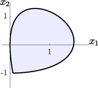
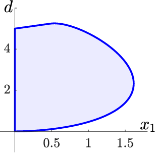
fig. 2.4 shows two-dimensional projections of the three-dimensional feasible set of the two LMIs in eq. 2.6. As expected, the projection on the plane coincides with the feasible set of LMI eq. 2.5, which is contained inside the thick black line in fig. 2.4(a). This confirms that the LMIs in eq. 2.6 are equivalent to the LMI eq. 2.5. Therefore, we have decomposed a LMI into two coupled LMIs of size .

2.2.3 Cone of positive-semidefinite-completable matrices
A concept related to the matrix decomposition above is that of positive semidefinite matrix completion. Given a matrix , let
| (2.7) |
be its projection onto the space of sparse matrices with respect to the Frobenius matrix norm. We define the cone
Using eq. 2.7, it is not hard to see that a sparse matrix is in if and only if it has a positive semidefinite completion, meaning that some (or all) of the zero entries with can be replaced with nonzeros to obtain a positive semidefinite matrix . We call the completion of and refer to as the cone of positive-semidefinite-completable matrices.
Remark 2.2 (Nonuniqueness of the positive semidefinite completion).
The positive semidefinite completion of a matrix with sparsity pattern is generally not unique. For a chordal sparsity pattern , two widely used and efficient strategies to compute a completion are the maximum determinant completion (Vandenberghe et al. 2015, Chapter 10.2), which maximizes , and the minimum rank completion (see Dancis 1992; Jiang 2017; Sun 2015), which minimizes . In particular, there exists a positive semidefinite completion whose rank agrees with the maximum rank of the principal submatrices (Dancis 1992, Theorem 1.5), i.e.,
| (2.8) |
For any undirected graph , the cones and are dual to each other with respect to the trace inner product in the space (Vandenberghe et al. 2015, Chapter 10). To see this, observe that
For a chordal matrix sparsity pattern, theorem 2.1 on the decomposition of the cone can be dualized to obtain the following characterization of , first proved by Grone et al. 1984.
Theorem 2.2.
Let be a chordal graph with maximal cliques . Then, if and only if
| (2.9) |
The “only if” part of theorem 2.2 is immediate, since any principal submatrix of a positive semidefinite matrix is positive semidefinite. The “if” part, instead, relies on the properties of chordal graphs and, as mentioned above, can be proven by combining the duality between and with theorem 2.1 (Vandenberghe et al. 2015, p. 357). Precisely,
The first equivalence expresses the duality between and , the second one follows from theorem 2.1, and the third one follows from the cyclic property of the trace operator: for any matrices of compatible dimensions.
fig. 2.5 illustrates how the duality between and is mirrored in the duality between theorem 2.1 and theorem 2.2 for chordal graphs.
Example 2.3.
Consider the symmetric matrix
whose sparsity pattern is the (by now usual) 3-node chordal chain graph with maximal cliques and . It is easy to check that, while is not positive semidefinite, the principal submatrices indexed by the cliques and are. Then, theorem 2.2 guarantees that , meaning that the zero entries may be replaced by nonzeros to obtain a positive semidefinite matrix . One possible positive semidefinite completion is
In fact, this is the minimum-rank completion whose rank, , coincides with the maximum rank of individual principal submatrices of (cf. Remark 2.2).
Example 2.4.
Consider the problem of finding a variable such that the matrix
| (2.10) |
admits a positive semidefinite completion. This is equivalent to finding as well as a corresponding scalar such that
| (2.11) |
Since the sparsity graph of is chordal, theorem 2.2 implies that eq. 2.10 is equivalent to the two LMIs
| (2.12) |
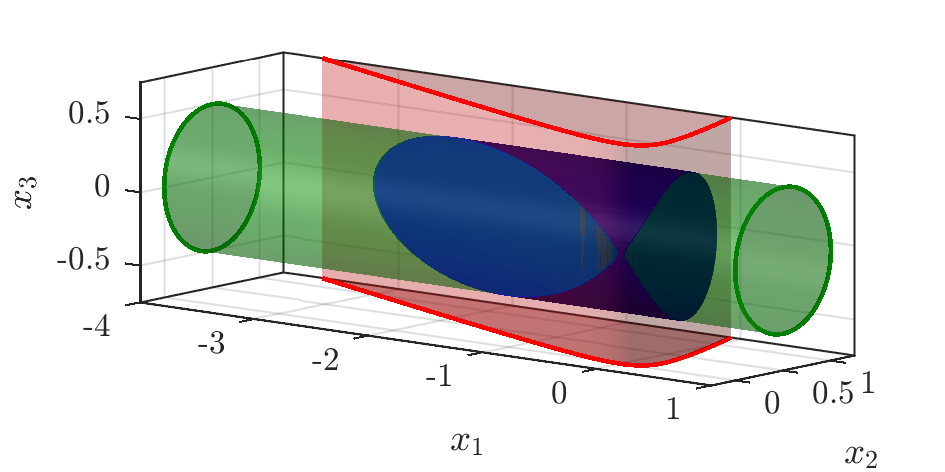
Feasible vectors for the first of these two LMIs can be found by imposing and , while feasible for the second LMI are found by requiring and . The feasible sets obtained in each case are illustrated by the red and green regions in Figure 2.6, respectively. The blue region in the figure, instead, represents the three-dimensional set of feasible for eq. 2.11. As expected from theorem 2.2, this is exactly the intersection of the feasible regions for the two LMIs in eq. 2.12. Similar to example 2.2, one can therefore replace the original completion constraint—which is equivalent to LMI eq. 2.11—with the two LMIs in eq. 2.12 without any loss of generality.
2.3 Block-partitioned matrices
Theorems 2.1 and 2.2 can be extended to block-partitioned matrices characterized by block-sparsity. Such matrices arise, for example, when modeling network systems (cf. Section 6.1), where each block in the partition corresponds to an individual subsystem and sparsity in the network connectivity translates into block-sparsity. Block-partitioned matrices are also useful in extending factor-width decomposition that will be discussed in Section 5.
2.3.1 Sparse block matrices
Given a positive integer , any finite set of positive integers is called a partition of if . The set of all possible partitions of can be equipped with the following (partial) order relation.
Definition 2.2.
Let and be two partitions of an integer with . We say that is finer than (and is coarser than ), denoted by , if there exist integers with , and for such that for all
Essentially, a finer partition breaks some entries of into smaller ones (conversely, a coarser partition is obtained by merging some entries of into a bigger one). For example, the partitions and of satisfy .
Given any integer and any partition of , a matrix can be written in the block form
with for all . For the finest partition , the block reduces to the entry of . As shown below and in section 5.3, however, the freedom to consider a nontrivial partition offers considerable flexibility when devising decomposition strategies for a large matrix . In particular, by refining or coarsening a partition one can in principle split a matrix into blocks of optimal size for the computational resources at one’s disposal.
The block sparsity pattern of an matrix whose blocks are defined by a partition of can be described using a graph with and edge set such that if , where is the -th block in and denotes a zero block of appropriate size. We call a chordal partition if the corresponding block sparsity graph is chordal. The linear space of sparse symmetric block matrices with a prescribed block sparsity pattern is then given by
The block-sparse positive semidefinite cone and the block-sparse positive-semidefinite-completable cone are simply
| (2.13a) | ||||
| (2.13b) | ||||
Remark 2.3 (Chordal partitions and chordal extension).
If is a sparse matrix with nonchordal sparsity pattern, it is often possible to find one or more chordal partitions . An example is the symbolic matrix
where the partitions and are both chordal (the corresponding block sparsity graphs are illustrated in fig. 2.7). For a given chordal partition, in this example but also in general, completing all blocks of that are not identically zero results in a chordal extension of . For instance, the chordal extension of the matrix above resulting from the partitions and are, respectively,
where entries colored in red have been added by the block-completion process. Finding a chordal partition for a matrix, therefore, gives a way of performing a particular chordal extension of its sparsity pattern. The opposite, however, is not true: not all chordal extensions are obtained via a block-completion operation. One example for the matrix above is the chordal extension
which is obtained by a symbolic Cholesky factorization with approximately minimal degree ordering.
2.3.2 Chordal decomposition of sparse block matrices
As anticipated above, decomposition results similar to theorems 2.1 and 2.2 hold for and when is a chordal partition of . Given a clique of the chordal block sparsity graph subordinate to the chordal partition , we define the block matrix , where , as
| (2.14) |
Here, is an identity matrix of dimension . When is the trivial partition, reduces to the matrix in eq. 2.2. Similar to the case studied in section 2.2, the operation extracts the principal block-submatrix of whose blocks are indexed by , while “inflates” an matrix into a sparse block matrix.
We are now ready to extend theorems 2.1 and 2.2 to the case of sparse block matrices.
Theorem 2.3 (Chordal block-decomposition).
Let be a chordal graph with maximal cliques , and let be a partition of . Then, if and only if there exist matrices for such that
| (2.15) |
Theorem 2.4 (Chordal block-completion).
Let be a chordal graph with maximal cliques , and let be a partition of . Then, if and only if
| (2.16) |
The proofs of theorems 2.3 and 2.4 rely on the fact that the block sparsity graph of induces a chordal extension of the standard sparsity graph of (cf. Remark 2.3) and, in fact, it is a hypergraph of the latter. The normal chordal decomposition and completion from theorems 2.1 and 2.2 can then be applied to the chordal extension of , and the hypergraph structure implies the two results above. Interested readers are referred to Zheng 2019 for details.
Example 2.5.
Consider the matrices
and
which have the same nonchordal sparsity pattern as the symbolic matrix considered in Remark 2.3. Readers can easily check that is positive semidefinite, while admits a positive semidefinite completion (e.g., replace all zero entries with ones to obtain ). The partitions and are both chordal, so while theorem 2.1 cannot be directly applied to decompose , theorem 2.3 guarantees the existence of decompositions either in the symbolic form
(corresponding to the partition ) or in the symbolic form
(corresponding to the partition ). These coincide with the classical chordal decompositions applied to the chordal extensions of from the chordal partitions and . Thus, one can choose whether to decompose as a sum of four matrices with nonzero principal submatrices, or as a sum of two matrices with nonzero principal submatrices. Similarly, one can apply theorem 2.4 to verify that the matrix admits a positive semidefinite completion by checking the positive semidefiniteness of either four principal submatrices, or two ones.
3 Sparse semidefinite optimization
The matrix decomposition and completion results in theorems 2.1 and 2.2 can be used to reduce the complexity of algorithms for sparse semidefinite optimization. A semidefinite program (SDP) in standard primal form takes the form
| (3.1) | ||||
where are the problem data. The dual problem to eq. 3.1 is also an SDP,
| (3.2) | ||||
In this section, we describe decomposition techniques for SDPs that exploit the joint sparsity pattern of the coefficient matrices , called aggregate sparsity pattern. For simplicity, we assume that the matrices are linearly independent and that there exist , and satisfying the equality constraints in eqs. 3.1 and 3.2. This ensures that the primal and dual optimal values are finite, equal, and attained. SDPs that are infeasible or have unbounded objective can be tackled using homogeneous self-dual embeddings (Ye et al. 1994; O’Donoghue et al. 2016; Ye 2011) or by analyzing the divergence of the iterates produced by solution algorithms (Liu et al. 2017; Banjac et al. 2019). Sparsity can be exploited within these frameworks, too, and we refer the interested reader to Zheng et al. 2020 and Garstka et al. 2019 for details.
3.1 Aggregate sparsity
The pair of SDPs eq. 3.1-eq. 3.2 is said to have aggregate sparsity graph if
| (3.3) |
Of course, if is an extension of , then is also a suitable aggregate sparsity graph. The minimal one, therefore, is simply the union of the individual sparsity graphs of , . Throughout this section, however, we consider a chordal extension of the minimal aggregate sparsity graph. We therefore assume from now on that the aggregate sparsity pattern is chordal and has maximal cliques .
It must be noted that an SDP may have a fully connected aggregate sparsity graph even if all coefficient matrices and are very sparse; see Zheng et al. 2018b for explicit examples. The decomposition methods described below cannot be applied to such problems. However, there are broad classes of SDPs for which the sparsity of the SDP data matrices can be expected to translate into very sparse aggregate sparsity graphs.
One such family consists of SDPs arising from relaxations of graph optimization problems and control problems over networks, which typically inherit the structure of the underlying network or graph. Notable examples include SDP relaxations of combinatorial graph optimization problems, such as Max-Cut (Goemans & Williamson 1995) and graph equipartition (Karisch & Rendl 1998), eigenvalue optimization problems over graphs (Boyd et al. 2004), analysis of linear networked systems (Mason & Papachristodoulou 2014; Zheng et al. 2018d; Deroo et al. 2015; Zheng et al. 2018c), sensor network localization (Kim et al. 2009; Nie 2009; So & Ye 2007), neural network verification in machine learning (Raghunathan et al. 2018; Batten et al. 2021), and the optimal power flow problem in electricity networks (Bai et al. 2008; Andersen et al. 2014a; Jabr 2011). We will briefly discuss some of these applications in Section 6.
Another source of SDPs with aggregate sparsity is the reformulation of intractable constraints (either convex or nonconvex) as tractable LMIs using auxiliary variables (Ben-Tal & Nemirovski 2001; Vandenberghe et al. 2015). For example, consider the uncountable family of “uncertain” convex quadratic constraints
on a variable , to be imposed for all matrices , vectors and scalars in the form
with . Here, , and are nominal reference values, and are fixed perturbations. Andersen et al. 2010b showed that this family of constraints is equivalent to a sparse LMI in the form
| (3.4) |
where while , and are known linear functions whose exact form is not important here. When , this matrix has a “block-arrow” aggregate sparsity pattern analogous to that shown in fig. 2.3 (that figure is recovered exactly when , , and is arbitrary). This particular type of sparsity pattern is commonly encountered in robust optimization (Goldfarb & Iyengar 2003; Ben-Tal & Nemirovski 1998; Andersen et al. 2010b).
Remark 3.1 (Promoting aggregate sparsity).
Sometimes, it is possible to reformulate SDPs with no aggregate sparsity as equivalent SDPs with very sparse aggregate sparsity graphs through a carefully chosen transformation of variables (Fukuda et al. 2001, Section 6; Vandenberghe et al. 2015, Chapter 14.1). For instance, the SDP relaxation of the graph equipartition problem studied by Fukuda et al. 2001 has sparse data matrices and , but the -th constraint destroys the problem’s aggregate sparsity because the matrix is dense. However, any matrix satisfying can be expressed as for some matrix , where
Thus, the original SDP can be reformulated as
where and . Since is a sparse basis matrix and the original data matrices are sparse, this new SDP is characterized by aggregate sparsity (Fukuda et al. 2001, Section 6). Sparsity-promoting modeling strategies that generalize this example are discussed by Vandenberghe et al. 2015.
| Reference | Chordal Sparsity | SDP Type | Algorithm | Infeas./ Unbounded | Solver |
| Wen et al. 2010 | ✗ | eq. 3.2 | ADMM | ✗ | ✗ |
| Zhao et al. 2010 | ✗ | eq. 3.2 | Augm. Lagrang. | ✗ | SDPNAL |
| O’Donoghue et al. 2016 | ✗ | eq. 3.1-eq. 3.2 | ADMM | ✓ | SCS |
| Yurtsever et al. 2021 | ✗ | eq. 3.11 | SketchyCGAL | ✗ | CGAL |
| Lu et al. 2007 | ✓ | eq. 3.1 | Mirror-Prox | ✗ | ✗ |
| Lam et al. 2012 | ✓ | OPF2 | Primal-dual | ✗ | ✗ |
| Dall’Anese et al. 2013 | ✓ | OPF2 | ADMM | ✗ | ✗ |
| Sun et al. 2014 | ✓ | Special3 | Gradient proj. | ✗ | ✗ |
| Sun & Vandenberghe 2015 | ✓ | eq. 3.1-eq. 3.2 | Spingarn | ✗ | ✗ |
| Kalbat & Lavaei 2015 | ✓ | Special4 | ADMM | ✗ | ✗ |
| Madani et al. 2017a | ✓ | General5 | ADMM | ✗ | ✗ |
| Zheng et al. 2020 | ✓ | eq. 3.1-eq. 3.2 | ADMM | ✓ | CDCS |
| Garstka et al. 2019 | ✓ | Quad. SDP6 | ADMM | ✓ | COSMO |
Note: 1. It requires an explicit trace constraint on ; 2. Special SDPs from the optimal power flow (OPF) problem; 3. Special SDPs from the matrix nearness problem; 4. Special SDPs with decoupled affine constraints; 5. General SDPs with inequality constraints; 6. A dual SDP eq. 3.2 with a quadratic objective function.
3.2 Nonsymmetric formulation
The aggregate sparsity of the primal-dual pair of SDPs eq. 3.1–eq. 3.2 can be exploited by reformulating them into a nonsymmetric pair of optimization problems, proposed by Fukuda et al. 2001 and later discussed extensively by Andersen et al. 2010a; Sun et al. 2014; Kim et al. 2011; Zheng et al. 2020.
Consider first the dual-standard-form SDP eq. 3.2. Any feasible matrix must be at least as sparse as the aggregate sparsity pattern of the SDP. We can therefore restrict to the subspace , where is the edge set of the aggregate sparsity graph, and rewrite eq. 3.2 as
| (3.5) | ||||
The primal-standard-form SDP eq. 3.1, instead, typically has a dense optimal matrix . However, the value of the cost function and the equality constraints depend only on the entries with , while the remaining ones simply guarantee that is positive semidefinite. We can therefore pose eq. 3.1 as an optimization problem over the cone of sparse matrix that admit a positive semidefinite completion,
| (3.6) | ||||
Problems eq. 3.6 and eq. 3.5 are a primal-dual pair of linear conic programs because the cones and are dual to each other (see section 2.2 and fig. 2.5). Even though the sparse matrix cones and are not self-dual (Andersen et al. 2010a; Andersen 2011), so this sparse formulation is nonsymmetric, one can solve eq. 3.6, eq. 3.5, or both problems simultaneously using a variety of first-order or interior-point algorithms. The next two subsections discuss some of them.
Remark 3.2.
A special type of aggregate sparsity arises when the data matrices are block-diagonal. In this case, any feasible matrix for eq. 3.6 is automatically positive semidefinite and, consequently, can be restricted to . Therefore, the nonsymmetric formulation described above becomes symmetric. In particular, problems eqs. 3.6 and 3.5 are simply SDPs with a Cartesian product of semidefinite cones, where is the size of the th diagonal block and is the number of blocks.
3.3 First-order algorithms
First-order optimization algorithms rely only on gradient information and have iterations with low computational complexity, which can often be implemented in a distributed manner (Boyd et al. 2011; Beck 2017). For these reasons, the last decade has witnessed the development of a range of first-order methods to solve large-scale SDPs, many of which are listed in table 1. Some of these methods (Wen et al. 2010; Zhao et al. 2010; O’Donoghue et al. 2016; Yurtsever et al. 2021) focus on generic SDPs and do not exploit aggregate sparsity. Others, instead, tackle the sparsity-exploiting nonsymmetric formulations eq. 3.5–eq. 3.6 using so-called domain space or range-space conversion frameworks, which replace the matrix cones and with smaller positive semidefinite cones using the chordal decomposition and completion results in theorems 2.1 and 2.2 (see, e.g., Lu et al. 2007; Lam et al. 2012; Dall’Anese et al. 2013; Sun et al. 2014; Sun & Vandenberghe 2015; Kalbat & Lavaei 2015; Madani et al. 2017a; Zheng et al. 2020; Garstka et al. 2019). Many of these works combine this strategy with additional separability assumptions for the equality constraints, which are satisfied in optimal power flow problems (Lam et al. 2012; Dall’Anese et al. 2013; Kalbat & Lavaei 2015) and the matrix nearness problems (Sun et al. 2014) but not in general. To the best of our knowledge, the only first-order methods that can currently handle general SDPs with aggregate sparsity (including infeasible or unbounded ones) are those developed by Zheng et al. 2020 and Garstka et al. 2019.
3.3.1 Domain- and range-space conversion
Consider problem eq. 3.6. When the aggregate sparsity graph is chordal and has maximal cliques , theorem 2.2 allows one to replace the constraint with
| (3.7) |
These constraints are coupled in general because the matrices and depend on the same entries of if the cliques and overlap. The works referenced above differ primarily in how these couplings are handled and, as discussed in remarks 3.3 and 3.5 below, the choice of strategy can have a considerable impact on the overall complexity of the iterations in a first-order method.
A simple but powerful strategy was proposed recently by Zheng et al. 2020, who used “slack” matrices to rewrite eq. 3.7 as
| (3.8) |
The primal SDP eq. 3.6 is then equivalent to
| (3.9) | |||||
Following Fukuda et al. 2001 and Zheng et al. 2020, we refer to eq. 3.9 as the domain-space decomposition of the primal SDP eq. 3.1.
A range-space decomposition of the dual SDP eq. 3.2 can be formulated in a very similar way. When the aggregate sparsity pattern is chordal, theorem 2.1 implies that the constraint is equivalent to
| (3.10) |
Observe that, as before, the first of these conditions couples the positive semidefinite matrices and if the cliques and of the aggregate sparsity graph overlap. To decouple them, Zheng et al. 2020 introduced slack variables and reformulated eq. 3.10 as
| (3.11) |
Using this to eliminate from eq. 3.5 yields the range-space decomposition
| (3.12) | ||||
While the domain- and range-space decompositions eq. 3.9 and eq. 3.12 have been derived independently, it is not difficult to verify that they are a primal-dual pair of SDPs. The duality between the original SDPs eq. 3.1 and eq. 3.2 is thus inherited by the decomposed SDPs eq. 3.9 and eq. 3.12 by virtue of the duality between Theorem 2.2 and Theorem 2.1. This elegant picture is illustrated in fig. 3.1.
Remark 3.3.
The introduction of variables and leads to redundancies in the affine constraints of eqs. 3.9 and 3.12, but is essential to obtain a decomposition framework that is suitable for the development of fast first-order SDP solvers. For example, as explained in section 3.3.2 below, applying the alternating direction method of multipliers (ADMM) to eq. 3.9 leads to an algorithm whose iterations have closed-form update rules that can be implemented efficiently. The same is usually not true if the redundant constraints in eq. 3.9 are used to eliminate the matrix : the iterations of the first-order method proposed by Sun et al. 2014, for instance, require the solution of a further SDP with quadratic objective function, which limits its scalability. However, the matrix may be eliminated from eq. 3.9 without compromising efficiency if the original primal SDP eq. 3.1 has separable affine constraints. This observation was exploited to solve sparse SDPs arising from optimal power flow problems (Kalbat & Lavaei 2015; Dall’Anese et al. 2013) and matrix nearness problems (Sun & Vandenberghe 2015). Similar observations apply to the seemingly redundant matrices in the range-space decomposed SDP eq. 3.12.
3.3.2 ADMM for decomposed SDPs
The alternating direction method of multipliers (ADMM) is a first-order operator-splitting method developed in the mid-1970s (Gabay & Mercier 1976; Glowinski & Marroco 1975) to solve general optimization problems in the form
| (3.13) | ||||
where and are proper convex (but not necessarily smooth) functions on finite-dimensional normed vector spaces and , and are given linear operators from and into a finite-dimensional normed vector space , and is given. Given a penalty parameter and a dual variable that acts as a Lagrange multilier for the equality constraint, ADMM finds a saddle point of the (scaled) augmented Lagrangian
by updating the primal variables , and the dual variable according to the following rules:
| (3.14a) | ||||
| (3.14b) | ||||
| (3.14c) | ||||
The superscript indicates that a variable is fixed to its value at the -th iteration. Under mild technical conditions (Boyd et al. 2011, Section 3.2), the method converges to an -approximate solution of eq. 3.13 using at most iterations.
Given its slow convergence rate, ADMM is suitable only when eq. 3.14a and eq. 3.14b have closed-form expressions and/or can be solved efficiently. Below, we show that this is true when the method is applied to the decomposed SDPs eqs. 3.9 and 3.12.
Domain-space decomposition
Consider the domain-space decomposition eq. 3.9. Let denote the characteristic function of a set , i.e.,
For simplicity, we write when . Problem eq. 3.9 is equivalent to
| subject to | ||||
Upon letting and , this problem may be written in the standard form eq. 3.13 over the spaces and , and can therefore be solved using ADMM. Introducing a penalty parameter and a dual variable , where each acts as a Lagrange multiplier for the corresponding constraint , it is not difficult to check that the ADMM step eq. 3.14a reduces to an equality-constrained quadratic program,
Step eq. 3.14b, instead, reduces to independent positive semidefinite projections of the form for
Finally, step eq. 3.14c updates the multipliers according to
These three steps have efficient closed-form solutions and can be implemented efficiently (Zheng et al. 2020, Section 4.1). In particular, the independent projections onto the cones required to compute can be computed through an eigenvalue decomposition with complexity of floating-point operations. This is not expensive when all cliques of the aggregate sparsity graph are small, which is often true in many applications. In contrast, the first-order algorithms for generic SDPs developed in Wen et al. 2010; O’Donoghue et al. 2016 require a projection onto the semidefinite cone at each iteration, which becomes a bottleneck when . It is therefore clear that exploiting sparsity via chordal decomposition can bring significant computational savings in ADMM algorithms.
Range-space decomposition:
The range-domain decomposition eq. 3.12 of the dual-standard-form SDP eq. 3.2 can be solved using an ADMM algorithm very similar to that presented above. First, observe that eq. 3.12 is equivalent to
| subject to | ||||
Grouping the variables as and , this problem can be written in the general form eq. 3.13 over the spaces and Given a penalty parameter and a dual variable , where each acts as a Lagrange multiplier for the corresponding constraint , one can easily verify that the ADMM step eq. 3.14a reduces to solving the equality-constrained quadratic program
| subject to | ||||
| Step eq. 3.14b, instead, reduces to independent positive semidefinite projections of the form | ||||
| (3.17) | ||||
| Finally, the dual variables are updated through step eq. 3.14c as | ||||
Again, these iterations admit inexpensive closed-loop expressions. Moreover, it is not difficult to see that the ADMM iterations for the range-space decomposition eq. 3.12 and for the domain-space decomposition eq. 3.9 have similar leading-order complexity. In fact, Zheng et al. 2020 showed that the ADMM algorithms for the primal and dual decomposed SDPs are scaled versions of each other. This shows that the duality picture of figs. 3.1 and 2.5 is reflected also at the algorithmic level.
Remark 3.4.
For all fixed penalty , the primal and dual ADMM algorithms outlined above converge to a solution of eq. 3.9 and eq. 3.12, respectively, provided that strict primal-dual feasibility conditions are satisfied (Boyd et al. 2011, Section 3.2). An efficient ADMM algorithm that can handle primal or dual infeasible problems was developed by Zheng et al. 2020, who considered the homogeneous self-dual embedding (Ye et al. 1994; O’Donoghue et al. 2016) of the domain-space decomposition eq. 3.9 and the range-space decomposition eq. 3.12.
Remark 3.5.
As anticipated in Remark 3.3, considering the variables and the constraints without eliminating any redundant variables is essential to obtain efficient ADMM iterations. This is because the conic constraints separate completely from the affine ones in eq. 3.9 when applying the splitting strategy of ADMM, making it easy to update each via simple projections onto positive semidefinite cones. Similarly, the redundant variables and the constraints in eq. 3.12 are essential to decouple the conic constraints from the affine ones, which enables one to handle positive semidefinite constraints via simple projections.
3.4 Interior-point algorithms
Interior-point algorithms for convex optimization problems with equality and inequality constraints employ Newton’s method to solve a sequence of modified equality-constrained problems, obtained by replacing any inequality constraints with barrier functions in the objective (Nesterov 2003; Ye 2011). These barrier functions approximate the characteristic function of the set defined by the original inequality constraints and ensure that the optimal solution of each modified problem is strictly feasible for the original problem, meaning that it is an interior point of the original feasible set.
Since Newton’s method relies on second-order (Hessian) information, interior-point algorithms do not share the slow convergence of first-order methods. Instead, they converge to an -approximate solution using at most Newton iterations (Nesterov 2003; Ye 2011). In practice, convergence often occurs within tens of iterations. Therefore, interior-point methods are typically preferred when solving eq. 3.1-eq. 3.2 to high accuracy. The general-purpose SDP solvers SeDuMi (Sturm 1999), SDPT3 (Tütüncü et al. 2003), SDPA (Yamashita et al. 2012), and MOSEK (Mosek 2015) are all based on primal-dual interior-point methods, and they can very reliably solve small and medium-sized SDPs (e.g., when is less than a few hundreds and is less than a few thousands in eq. 3.1-eq. 3.2) on regular computers. However, they become impractical for large SDPs because the CPU time and memory requirements for each interior-point iteration increase as and , respectively (Nesterov 2003, Section 4.3.3).
Chordal graph techniques can be exploited to improve the efficiency of interior-point methods when solving large-scale SDPs with chordal aggregate sparsity (Fukuda et al. 2001; Andersen 2011; De Klerk 2010). This section reviews two general approaches for doing so. The first one, similar to the conversion methods in section 3.3.1, reformulates problems eqs. 3.6 and 3.5 as SDPs with small positive semidefinite cones, which are often easier to solve with general-purpose interior-point solvers (Fukuda et al. 2001; Nakata et al. 2003; Kim et al. 2011; Zhang & Lavaei 2020b). The second approach, instead, directly solves eq. 3.6-eq. 3.5 using an interior-point method for nonsymmetric conic optimization (Andersen et al. 2010a; Nesterov 2012; Skajaa & Ye 2015; Coey et al. 2020). For other ways to exploit chordal sparsity in the computation of interior-point search directions, we refer the reader to the works by (Benson et al. 2000), Pakazad et al. 2017b and Fukuda et al. 2001.
3.4.1 Conversion methods
Starting from the domain-space decomposed SDP eq. 3.9, Fukuda et al. 2001 and Kim et al. 2011 suggested to eliminate the global matrix and rewrite the SDP eq. 3.6 only in terms of variables . To rewrite the cost function and the first set of equality constraints, one must choose matrices and that satisfy
and
These affine relations do not usually determine and uniquely, and some choices may be more convenient than others from the point of view of computations (Sun et al. 2014, Section 3.1, Zhang & Lavaei 2020b, Section 6). The second set of constraints in eq. 3.9, instead, can be enforced via consistency constraints on the entries of that correspond to the same elements of . Such consistency constraints can be formulated as
| (3.18) | ||||
The primal SDP eq. 3.6 can therefore be rewritten as
| (3.19) | ||||
This conversion process, first proposed in Fukuda et al. 2001, is known as the domain-space decomposition (Kim et al. 2011). The reformulated problem eq. 3.19 has more variables and constraints than the original SDP eq. 3.1, but the large matrix constraint is replaced by smaller ones, for . In certain cases, the decomposed problem eq. 3.19 is easier to solve than the original SDP eq. 3.1 using general-purpose interior-point solvers; see Nakata et al. 2003 and Fujisawa et al. 2009 for numerical examples. Three other variants of this conversion method, including range-space decompositions, have been studied by Kim et al. 2011.
The main drawback of these conversion methods is that, sometimes, the additional consistency constraints eq. 3.18 significantly increase the size of the Schur complement system that needs to be solved at each interior-point iteration. This can offset the benefits of the clique-based matrix decomposition. As shown recently by Zhang & Lavaei 2020b, this issue can be mitigated using a dualization technique (Löfberg 2009).
Remark 3.6 (Removing redundant constraints).
Since the maximal cliques in a chordal graph satisfy the running intersection property (Blair & Peyton 1993; Fukuda et al. 2001) (see also appendix C), it is in fact sufficient to enforce the consistency between pairs that correspond to the parent-child pairs in a clique tree. Redundant constraints in eq. 3.18 can therefore be removed using the running intersection property. Interested readers are referred to Kim et al. 2011 and Vandenberghe et al. 2015 for details.
Remark 3.7 (Dropping or fixing consistency constraints).
In some applications, the SDP eq. 3.1 comes from a semidefinite relaxation of a nonconvex optimization problem. Dropping some consistency constraints in eq. 3.18 leads to a valid weaker relaxation with a lower computational complexity. This idea was successfully applied to semidefinite relaxations for optimal power flow problems (Andersen et al. 2014a) and neural network verification (Batten et al. 2021). Other times, one can enforce some of the consistency conditions a priori and look for feasible (but suboptimal) points for an SDP at a low computational cost. This idea was used in Zheng et al. 2018d to develop a scalable approach for solving distributed control problems.
3.4.2 Nonsymmetric interior-point algorithms
Chordal graph techniques can also be exploited to speed up interior-point methods for the nonsymmetric pair of sparse SDPs eq. 3.6-eq. 3.5 without appealing to the matrix decomposition and conversion frameworks described above. Since the cones and are not self-dual, such sparsity-exploiting methods cannot enjoy a complete primal-dual symmetry (Andersen et al. 2010a). Instead, one must resort to purely primal, purely dual, or nonsymmetric primal-dual path-following methods (Andersen et al. 2010a; Nesterov 2012; Skajaa & Ye 2015; Burer 2003; Coey et al. 2020).
To construct nonsymmetric interior-point methods, Dahl et al. 2008 and Andersen et al. 2010a introduced barrier functions and for the cones and , defined as
| (3.20a) | |||
| and | |||
| (3.20b) | |||
Note that (resp. ) is finite only on the interior of (resp. ) and tends to as (resp. ) approaches the boundary of this cone. Observe also that is simply the Legendre transform of evaluated at .
Thanks to the properties of the barrier functions, a minimizing sequence for eq. 3.6 can be computed by solving the regularized primal problem
| (3.21) | ||||
and letting . Similarly, a minimizing sequence for eq. 3.5 is found upon solving the regularized dual problem
| (3.22) | ||||
for . Solutions of the regularized problems for fixed finite are usually found using Newton’s method, leading to so-called primal scaling and dual scaling interior-point methods. Other methods can also be used; for instance, Jiang & Vandenberghe 2021 recently suggested solving eq. 3.21 with a Bregman first-order method, where the complexity of evaluating the Bregman proximal operator can be reduced using a sparse Cholesky factorization.
When Newton’s method is applied to eq. 3.21, the KKT optimality conditions are
| (3.23a) | ||||
| (3.23b) | ||||
| (3.23c) | ||||
where is a Lagrange multiplier for the equality constraint in eq. 3.21 and is an auxiliary variable arising from the definition of via the Legendre transform. Solutions as is varied define the so-called central path for eq. 3.6. Similarly, the KKT optimality conditions for eq. 3.22 are
| (3.24a) | ||||
| (3.24b) | ||||
| (3.24c) | ||||
where is a Lagrange multiplier for the equality constraint in eq. 3.22. Solutions as is varied define the central path for eq. 3.5. It is possible to show that eq. 3.23 and eq. 3.24 are equivalent (Andersen 2011, Chapter 3), so the set of points in define a primal-dual central path.
The rest of this section briefly outlines how the chordality of the sparsity pattern can be exploited in the context of dual-scaling interior point methods. Similar ideas can be used to formulate primal-scaling methods, and we refer interested readers to the work by Andersen et al. 2010a for details.
Dual-scaling interior-point methods
Search directions in a dual-scaling interior-point method are obtained by linearizing eq. 3.24 around the current interior iterate , and . Replacing , and with , , in eq. 3.24, linearizing eq. 3.24c, and eliminating yields the Newton equations
| (3.25) | ||||
where is the inverse Hessian of at , and Further elimination of leads to the Schur complement equation
| (3.26) |
where is a vector and is an positive definite matrix, both depending only on the current (known) iterates , and . Explicit expression for these quantities are given by Andersen et al. 2010a.
Finding the dual-scaling search direction requires solving the Newton equation eq. 3.25 or the Schur complement equation eq. 3.26. To do this using a direct method, one must first calculate the Hessian and inverse Hessian of the barrier function in eq. 3.20a, and then form and factorize the matrix . This is the most computationally expensive part of any interior-point method. It is in this computation that one can exploit the chordality of the sparsity pattern (Andersen et al. 2010a).
Fast calculations involving the barrier functions
The value, gradient, Hessian, and inverse Hessian of the dual barrier in eq. 3.20a can be computed efficiently if the sparsity pattern of is chordal. Similar fast algorithms exist for the primal barrier in eq. 3.20b, but we do not review them here and refer interested readers to Andersen et al. 2010a for details.
The key ingredient of these efficient algorithms is a sparse Cholesky factorization with zero fill-in (Rose 1970; Blair & Peyton 1993; Vandenberghe et al. 2015): as reviewed in appendix A, for any positive definite matrix in with chordal sparsity there exists a permutation matrix and a lower triangular matrix such that
| (3.27) |
This factorization can be computed efficiently by following a recursion on a clique tree (Vandenberghe et al. 2015, Chapter 9.3).
Now, to evaluate it suffices to substitute into eq. 3.20a and observe that
because determinants distribute over products and permutation matrices have unit determinant. Thus, can be evaluated efficiently once the Cholesky factorization eq. 3.27 has been computed.
The gradient of , instead, is given by the following negative projected inverse
Despite the fact that is in general dense, the projection onto can be computed from its sparse Cholesky factorization eq. 3.27 without computing any other entries of (Vandenberghe et al. 2015, Chapter 9.5).
The Hessian of at applied to a matrix is computed as
Again, this quantity can be evaluated knowing only the sparse Cholesky factorization of and its projected inverse , without explicitly computing the inverse or the matrix product (Andersen et al. 2010a; Andersen et al. 2013).
Finally, thanks to the chordal structure, solving the linear equation for in order to evaluate the inverse Hessian has the same cost as the evaluating the Hessian ; see Andersen et al. 2010a and Andersen et al. 2013.
3.5 Algorithm implementations
We conclude this section by providing a list of numerical packages that implement some of the approaches reviewed above. This list is not exhaustive, and the goal here is to give the interested reader a starting point for numerical experiments. First-order solvers based on augmented Lagrangian methods and ADMM for generic SDPs include SDPNAL/SDPNAL+ (Sun et al. 2020; Zhao et al. 2010) and SCS (O’Donoghue et al. 2019). CDCS (Zheng et al. 2016) and COSMO (Garstka et al. 2019) are two open-source first-order solvers that exploit chordal sparsity in SDPs. The MATLAB package CDCS implements the algorithms described in Section 3.3.2 and has interfaces with the optimization toolboxes YALMIP (Löfberg 2004) and SOSTOOLS (Prajna et al. 2002). The Julia package COSMO solves SDPs with quadratic objective functions.
The conversion methods in Section 3.4.1 are implemented in SparseCoLO (Fujisawa et al. 2009) and CHOMPACK (Andersen & Vandenberghe 2015). We note that CHOMPACK also provides useful implementation of many other chordal matrix computations, including maximum determinant positive definite completion and minimum rank positive semidefinite completion. Another MATLAB package Dual-CTC (Zhang & Lavaei 2020a) implements a dualized clique tree conversion (Zhang & Lavaei 2020b). The reformulated SDPs after conversion can be solved using general-purpose interior-point solvers, such as SeDuMi (Sturm 1999), SDPT3 (Tütüncü et al. 2003), SDPA (Yamashita et al. 2012), and MOSEK (Mosek 2015). SMCP (Andersen & Vandenberghe 2014) is a nonsymmetric interior-point solver that provides a Python implementation of the algorithms in Section 3.4.2. Finally, SDPA-C (Fujisawa et al. 2004) is a primal-dual interior-point solver that exploits chordal sparsity using the maximum-determinant positive definite completion.
4 Sparse polynomial optimization
We have seen in section 3 that the chordal decomposition of large semidefinite matrices allows for significant efficiency gains in the solution of sparse SDPs. The same ideas can often be leveraged to replace SDP relaxations of intractable optimization problems, which generally have no inherent sparsity or other computationally advantageous structure, with SDPs that do.
This section describes how sparsity (primarily chordal, but also nonchordal) can be exploited in the context of sum-of-squares (SOS) relaxation techniques for polynomial optimization. As mentioned in the introduction, SOS methods are at the heart of many recent tractable frameworks for the analysis and optimal control of nonlinear systems with polynomial dynamics; see Lasserre et al. 2008; Valmorbida & Anderson 2017; Henrion & Korda 2014; Lasagna et al. 2016; Jones & Peet 2019; Majumdar et al. 2014; Han & Tedrake 2018; Fantuzzi et al. 2016; Fantuzzi & Goluskin 2020; Goluskin 2020; Korda et al. 2021; Miller et al. 2021; Ahmadi & Gunluk 2018; Papachristodoulou & Prajna 2005; Prajna et al. 2004 to name but a few contributions.
Our goal is not to offer an exhaustive review of all sparsity-exploiting methods that have been proposed in this field, but rather to introduce the key ideas underpinning most of these methods from a general perspective, in the hope that this can guide further developments. For this reason, we concentrate mainly on two basic problems. The first, discussed in section 4.2, is to prove that an -variate polynomial of even degree is a sum of squares and, therefore, globally nonnegative. In this case, we seek to exploit the structure of polynomials that depend only a small subset of all possible degree- monomials—a property often referred to as term sparsity. The second problem, discussed in section 4.3, is to check whether a sparse and symmetric -variate polynomial matrix is SOS, and therefore positive semidefinite for all . In this case, our goal is to leverage the structural sparsity of , meaning that many of its entries are zero.
Although we focus only on global nonnegativity, all of the sparsity-exploiting techniques discussed in this section can be extended to prove polynomial (matrix) nonnegativity locally on basic semialgebraic sets. Such extensions, which have been studied extensively in order to build hierarchies of sparse SDP relaxations for polynomial optimization problems (Waki et al. 2006; Waki et al. 2008; Lasserre 2006; Wang et al. 2021b; Wang et al. 2021a; Wang et al. 2020a; Zheng & Fantuzzi 2020), require some careful technical adjustments, but the underlying strategy is the same as for the global nonnegativity setting. We outline some of these adjustments in sections 4.2.5 and 4.3.2, and refer readers to the excellent literature on this topic for full details.
4.1 Background
Let be the -dimensional space of polynomials with independent variables and degree no larger than . The -variate monomial with exponent and degree is denoted by . Given a finite set of exponents , we write for the (column) vector of monomials with exponents in . The cardinality of is denoted by . We also define
| (4.1a) | ||||
| (4.1b) | ||||
If is the set of all -variate exponents of degree or less, the vector is a basis for and any polynomial can be written as for some coefficients . The set of exponents with nonzero coefficient,
| (4.2) |
is called the support of . Its convex hull is called the Newton polytope of and is denoted by .
4.1.1 SOS polyonomials and SDPs
A polynomial of even degree is SOS if there exist degree- polynomials such that
| (4.3) |
The set of -variate degree- SOS polynomials, denoted by , is a proper cone in (Blekherman et al. 2012, Theorem 3.26). Given an exponent set , we define the subcone of SOS polynomials supported on as
| (4.4) |
It is well known (see, e.g., Parrilo 2003; Parrilo 2013) that a polynomial is SOS if and only if there exist a set of exponents and a positive semidefinite matrix such that
| (4.5) |
In particular, if is SOS, this so-called Gram matrix representation eq. 4.5 is guaranteed to exist with (Reznick 1978)
| (4.6) |
The exponent set obtained with this Newton polytope reduction can be simplified further using more general facial reduction techniques (Löfberg 2009; Permenter & Parrilo 2014a; Permenter & Parrilo 2014b; Waki & Muramatsu 2010). These techniques analyze the support of in order to remove redundant elements from , and construct a smaller exponent set for which eq. 4.5 is guaranteed to hold as long as is SOS.
It is clear that SOS polynomials are nonnegative globally. The converse is true only for univariate polynomials (, arbitrary), quadratic polynomials (, arbitrary), and bivariate quartics (, ) (Hilbert 1888). In general, therefore, being SOS is only a sufficient condition for global nonnegativity, and there are well-known examples of nonnegative polynomials that are not SOS, such the Motzkin polynomial (Motzkin 1967). However, while verifying polynomial nonnegativity is an NP-hard problem (Murty & Kabadi 1987), checking whether a polynomial is SOS can be done in polynomial time by solving an SDP. Specifically, for each exponent , let be the symmetric binary matrix satisfying
| (4.7) |
and observe that
| (4.8) |
Then, condition eq. 4.5 holds if and only if for all and we conclude that
| (4.9) |
The condition on the right-hand side defines an SDP, so a positive semidefinite Gram matrix certifying that is SOS can (in principle) be constructed in polynomial time.
4.1.2 SOS polynomial matrices and SDPs
Let be the space of matrices whose entries are -variate polynomials of degree . We say that a symmetric polynomial matrix is positive semidefinite (resp. definite) globally if (resp. ) for all . We also say that is positive semidefinite locally on a set if the same conditions hold for , but not necessarily otherwise.
A symmetric polynomial matrix is called SOS if there exists an integer and a polynomial matrix such that
| (4.10) |
The set of SOS polynomial matrices with entries in will be denoted by . All SOS polynomial matrices are clearly positive semidefinite globally, and the converse is true in the univariate case (); see Aylward et al. 2007 for a recent proof.
It is well known (see, e.g., Kojima 2003; Parrilo 2013; Gatermann & Parrilo 2004) that a symmetric polynomial matrix is SOS if and only if it admits a Gram matrix representation in the form
| (4.11) |
for some exponent set and some positive semidefinite symmetric matrix . One may always take , and smaller exponent sets can be constructed with the same reduction techniques used for SOS polynomials. As in the scalar case (), condition eq. 4.11 defines a set of affine constraints on , so verifying that a polynomial matrix is SOS amounts to solving an SDP.
4.2 Sparse SOS decompositions
A major obstacle to constructing SOS certificates of global polynomial nonnegativity via semidefinite programming is that the matrix is both dense and very large. If has dense support , then one must take and is a dense matrix. Often, however, the support of is small, i.e., is much smaller than . This property, called term sparsity (Wang et al. 2019; Wang et al. 2020a; Wang et al. 2021b; Wang et al. 2021a), can be exploited in various ways to reduce the computational complexity of the SDP in eq. 4.9.
The facial reduction techniques mentioned above, which replace the full exponent set with a (sometimes significantly) smaller subset, are arguably the simplest way to exploit term sparsity. However, as the next example demonstrates, they are often not sufficient.
Example 4.1.
Fix and . The support of
| (4.12) |
contains only out of the possible monomials, so is term sparse. However, it is not hard to check that the Newton polytope consists of all points with , so the Newton-reduced exponent set contains all homogeneous exponents of degree . Therefore, Newton polytope reduction removes only of the possible in the full set , and the SDP in eq. 4.9 still involves a Gram matrix .
Techniques to exploit term sparsity beyond what can be achieved with facial reduction methods alone are clearly desirable. Section 4.2.1 describes a general strategy to search for sparse SOS decompositions, which is based on the same matrix decomposition approach used to tackle large-scale sparse SDPs in section 3. Sections 4.2.2 and 4.2.3 show that different types of sparse SOS decompositions proposed in the literature are particular cases of this general approach. Section 4.2.5 outlines how these methods can be extended to prove polynomial nonnegativity on basic semialgebraic sets, rather than globally. Throughout, will denote a fixed set of candidate exponents for the SOS decomposition of a polynomial , generated from using facial reduction or any other exponent selection technique.
4.2.1 General approach
Let be a small subset of and be a term-sparse polynomial supported on . To reduce the cost of testing if is SOS, a natural idea is to check whether belongs to a subset of the sparse SOS cone that admits a semidefinite representation with low computational complexity. Such a subset can be constructed using a simple strategy: prescribe a sparsity graph for the Gram matrix and impose its positive semidefiniteness through matrix decomposition.
Precisely, let be a graph with maximal cliques and with edge set satisfying
| (4.13) |
Consider the cone of sparse SOS polynomial whose Gram matrix has sparsity graph and admits the clique-based positive semidefinite decomposition
| (4.14) |
We denote this cone by
| (4.15) |
Conditions eq. 4.13 and eq. 4.14 imply that . Moreover, inserting the clique-based decomposition eq. 4.14 of into eq. 4.9 one finds that if and only if
| (4.16) | ||||
If the cliques of the prescribed sparsity graph are small, the right-hand side is an SDP with small semidefinite cones and can be solved more efficiently than eq. 4.9.
Remark 4.1 (Chordality of the sparsity graph).
The Gram matrix decomposition eq. 4.14 is motivated by the chordal decomposition result in theorem 2.1. However, we do not assume here that the sparsity graph is chordal, so eq. 4.14 is generally not equivalent to requiring . The lack of chordality makes searching for the maximal cliques an NP-hard problem (Tomita et al. 2006). Allowing for nonchordal graphs with small cliques that can be determined analytically, however, can be extremely useful when a chordal extension leads to unacceptably large cliques even if it is approximately minimal. Examples of this situation can be found in works by Nie & Demmel 2009 and Kočvara 2020.
Remark 4.2 (Sparse SOS decompositions).
Given a sparsity graph , the cone contains special SOS polynomials that admit a sparse SOS decomposition, i.e., a decomposition into a sum of sparse SOS polynomials. Indeed, substituting eq. 4.14 into eq. 4.5 yields
| (4.17) |
Each polynomial is SOS because is positive semidefinite, and is sparse because the operation extracts a subset of the full monomial vector .
It is important to observe that the reduction in computational complexity granted by the clique-based decomposition eq. 4.14 usually comes at the expense of conservatism. This is because sparsity in the support set does not guarantee the existence of a sparse Gram matrix . For a given support set , special choices of the sparsity graph may ensure that (Zheng & Fantuzzi 2020, Corollaries 4.1 & 4.2; Mai et al. 2020, Theorem 2.1; Wang et al. 2019, Theorem 4.1; Wang et al. 2021b, Theorem 3.3). In general, however, sparse SOS polynomials need not admit a sparse SOS decomposition, so the inclusion is strict. The next example illustrates this.
Example 4.2.
(Klep et al. 2019, Lemma 5.2) Consider the polynomial and set . Let be the exponent set such that , which is obtained via Newton polytope reduction. Consider also the (chordal) sparsity graph shown in fig. 4.1, which satisfies eq. 4.13. We claim that belongs to but not to . To see this, observe that any Gram matrix representation of must take the form
where can be chosen arbitrarily. Setting makes the Gram matrix positive semidefinite, so . However, cannot be in because this would require , for which is not positive semidefinite.
4.2.2 Correlative sparsity
The general approach presented in Section 4.2.1 requires specifying the sparsity graph for the Gram matrix in eq. 4.5. A natural strategy to do this, pioneered by Waki et al. 2006 and Lasserre 2006, is to consider the couplings between any two independent variables and in a polynomial supported on . Two variables and are considered coupled if a monomial in the vector depends on both simultaneously, i.e., if there exists with . These couplings can be described using the correlative sparsity (csp) graph of the support set (or, alternatively, of the polynomial ), which has vertices and edge set
| (4.18) |
Correlatively sparse SOS decompositions are obtained upon imposing that the entry of the Gram matrix in eq. 4.5 vanishes if the monomial introduces couplings between variables that are not consistent with the csp graph of . This amounts to requiring that has sparsity graph with edge set
| (4.19) |
One may consider a “hypergraph” with nodes, built from the csp graph of (which has nodes) to ensure that polynomials with inherit the correlative sparsity of the original support set . Unsurprisingly, therefore, the properties of can be inferred from those of the (usually much smaller) csp graph. In the following statement, which can be proved using arguments similar to those given by Zheng 2019, denotes the indices of the nonzero entries of an exponent .
Proposition 4.1.
Suppose that the csp graph of the support set has maximal cliques . Then, has maximal cliques for . Moreover, if the csp graph of is chordal, then so is .
Proposition 4.1 considerably simplifies the construction of the “inflation” matrices in eq. 4.14, because it suffices to find the maximal cliques of the csp graph of without building the (much larger) graph . In addition, it is not difficult to check that the operation extracts monomials that depend only on variables indexed by . Using eq. 4.17, one concludes that exploiting correlative sparsity amounts to searching for a sparse SOS decomposition in the form
| (4.20) |
where denotes the subset of variables indexed by (cf. Zheng et al. 2019a, Theorem 2).
Remark 4.3.
Example 4.2 shows that correlatively sparse SOS polynomials need not admit the sparse SOS decomposition eq. 4.20, even if the csp graph is chordal. Thus, the inclusion is generally strict. For further discussion on the existence of sparse SOS decompositions for polynomials with chordal correlative sparsity, see Mai et al. 2020 and Zheng & Fantuzzi 2020.
Example 4.3.
The quartic polynomial in eq. 4.12 is correlatively sparse, and the csp graph of its support is chordal with maximal cliques for . It is clear that admits a sparse SOS decomposition eq. 4.20 and this can be searched for by solving the SDP in eq. 4.16. Since, for each clique , only six elements in can be multiplied together without introducing spurious couplings to different cliques, this SDP has semidefinite matrix variables . Its computational complexity is clearly much lower than the corresponding dense formulation in example 4.1, and a sparse SOS decomposition for can be found in less than one second on a standard laptop.
Example 4.4.
Consider the quartic polynomial
Its csp graph, shown in fig. 4.2(a), is nonchordal and has maximal cliques , , and . The corresponding graph , where the set of exponents obtained with Newton polytope reduction is , is shown in fig. 4.2(b) and has cliques containing elements each, which are determined using proposition 4.1. The sparsity pattern of the Gram matrix induced by and the clique-based matrix decomposition in eq. 4.14, also illustrated in the figure, replaces a positive semidefinite contraint on with four semidefinite constraints on matrices . According to eq. 4.20, searching for these matrices is equivalent to looking for a sparse SOS decomposition . Such a decomposition is not guaranteed to exist even if were SOS, but it does for this example with
This proves that .
4.2.3 TSSOS, chordal-TSSOS and related hierarchies
Fix an exponent set and a polynomial with . Correlative sparsity exploits only the sparse couplings between variables as encoded by the csp graph of , but does not take into account any further structure of . This is not efficient when is much smaller than , so is term-sparse, but the csp graph is fully connected or nearly so.
For this reason, Wang et al. 2019; Wang et al. 2021b; Wang et al. 2021a introduced the term-sparse-SOS (TSSOS) and the chordal-TSSOS decomposition hierarchies, which exploit term sparsity irrespective of whether is correlatively sparse. These are two particular examples of a broader family of possible sparsity-exploiting SOS decomposition hierarchies, each of which is obtained upon imposing the clique-based Gram matrix decomposition eq. 4.14 for a sequence of increasingly connected sparsity graphs ().
Irrespective of the particular hierarchy being considered (TSSOS, chordal-TSSOS, or another), the construction of such sparsity graphs begins with the observation that, in order to ensure eq. 4.13, each edge set should contain at least all edges with . This guarantees that for any Gram matrix defined via the clique-based decomposition eq. 4.14, which is necessary for the feasibility of the SDP in eq. 4.16. One should also not force diagonal entries of the Gram matrix to vanish, because this amounts to saying that the monomial is redundant and could be removed from the exponent set . For these reasons, we define an initial exponent set and an initial edge set as
| (4.21a) | |||
| (4.21b) | |||
Next, consider an extension operator which extends a given edge set according to a given rule. The edge sets and their corresponding support sets are defined using the iterative rule
| (4.22a) | ||||
| (4.22b) | ||||
Note that , so the extension operator guarantees that . Moreover, the sequence must converge to an edge set in a finite number of iterations because cannot be extended beyond the complete edge set . The sequence of sparsity graphs obtained in this way is therefore finite, and yields the (finite) hierarchy of nested sparse SOS cones
| (4.23) |
Here, is as defined in eq. 4.15 and all inclusions are strict in general.
Different extension operators produce different types of sparse SOS decomposition hierarchies. In particular:
- •
If is a block-completion operator that completes all connected components of the edge set , one recovers the TSSOS hierarchy (Wang et al. 2019; Wang et al. 2021b). At each step of the hierarchy, has chordal sparsity (specifically, a block-diagonal structure) and eq. 4.14 is equivalent to imposing .
- •
If is an approximately minimal chordal extension operator that extends the edge sets such that is chordal, one recovers the chordal-TSSOS hierarchy (Wang et al. 2021a). At each step of the hierarchy, has chordal sparsity and eq. 4.14 is equivalent to requiring .
In both cases, the edge extensions are performed on a graph with nodes and the maximal cliques of must be found at each iteration. This is unlike the correlative sparsity strategy in section 4.2.2, where the maximal cliques of are built from those in the csp graph of , which has only nodes (cf. proposition 4.1).
It is also clear that the choice of extension operator determines the computational complexity of the resulting sparse SOS decomposition hierarchy, as well as the gap between and . For example, the chordal-TSSOS hierarchy has a lower complexity than the TSSOS one in general, as its sparsity graphs have fewer edges (see Wang et al. 2021b; Wang et al. 2021a for detailed complexity estimates). However, the TSSOS hierarchy has a higher representation power because , which is generally not true for the chordal-TSSOS hierarchy.
Theorem 4.1 (Wang et al. 2021b).
If is the stabilized edge set of the TSSOS hierarchy, then , i.e., is SOS if and only if .
Remark 4.4.
Theorem 4.1 follows from a stronger result (Wang et al. 2021b, Theorem 6.5) which reveals that the constraint imposes the well-known block-diagonal structure implied by the sign symmetries of (see, e.g., Löfberg 2009).
Example 4.5.
The trivariate quartic polynomial
is term sparse but not correlatively sparse, since its csp graph is a complete graph with three nodes. The candidate exponent set to search for an SOS decomposition of is , as Newton polytope reduction removes no terms. For convenience, we order such that
The TSSOS hierarchy yields the sparsity graphs shown in fig. 4.3, which stabilize at the second iteration (). The corresponding sparsity patterns of the Gram matrix are also shown in that figure. Observe how the connected components of the initial graph are completed at the first iteration to obtain the graph . As discusses in Remark 4.4, the stabilized block-diagonal structure of coincides with the partition of into the groups , , and implied by the sign symmetries of , which is invariant under the transformations and (the four groups of monomials are invariant under both, the first, the second, and none of these transformations). In this example, the SDP in eq. 4.16 is feasible at all iterations of the TSSOS hierarchy because admits the positive semidefinite Gram matrix representation
and the Gram matrix is consistent with the sparsity graphs in fig. 4.3. Thus, all steps of the TSSOS hierarchy are able to prove that is SOS. Note that this can be guaranteed a priori only for the last step by virtue of theorem 4.1.
For the same polynomial , the chordal-TSSOS hierarchy stabilizes at the first iteration () and yields the sparsity graph shown in fig. 4.4. The corresponding Gram matrix is sparser than those encountered in the TSSOS hierarchy, leading to smaller semidefinite constraints in eq. 4.16. Again, this SDP is feasible in light of the Gram matrix decomposition given above, so the chordal-TSSOS hierarchy is able to prove that is SOS. This, however, cannot be guaranteed a priori.
Remark 4.5.
The explicit Gram matrix decomposition in example 4.5 reveals that the smaller monomial basis would suffice to construct an SOS decomposition of . It remains to be seen whether this reduced basis can be identified using strategies that are more sophisticated than the Newton polytope reduction.
4.2.4 Correlatively term-sparse hierarchies
The sparse SOS decomposition hierarchies described in section 4.2.3 can be combined with the correlative sparsity techniques outlined in section 4.2.2 in a natural way. Let be the edge set obtained using the iterations in eq. 4.22 for a given extension operator, and let be the edge set in eq. 4.19 constructed using correlative sparsity. Then, the sequence of sparsity graphs
| (4.24) |
yields a hierarchy of “correlatively term-sparse” SOS decompositions, which exploit simultaneously term and correlative sparsity. Since by construction, and since the sequence stabilizes onto an edge set in a finite number of steps, the sparse SOS cones corresponding to this hierarchy satisfy
and all inclusions are generally strict. Note also that one may remove from all exponents that violate the correlative sparsity before constructing the edge sets , because the intersection with eliminates all edges between such exponents (including self-loops).
When the extension operator used to build is the block-completion operation used in the TSSOS hierarchy, the sparsity graphs in eq. 4.24 yield exactly the CS-TSSOS hierarchy introduced by Wang et al. 2020a. In this case, by theorem 4.1, the stabilized sparsity graph simply encodes sign symmetries and correlative sparsity. Since exploiting sign symmetries in SOS decompositions brings no conservatism (Löfberg 2009), one immediately obtains the following corollary.
Proposition 4.2.
If is the stabilized edge set of the TSSOS hierarchy, then for any exponent set .
Example 4.6.
(Wang et al. 2020a, Example 3.4) Let
| (4.25) |
This polynomial is both term and correlatively sparse, and its csp graph has two maximal cliques and . It is also invariant under the sign symmetry transformation . To search for an SOS decomposition of using the CS-TSSOS hierarchy, we let be the exponent set defining the monomial vector
This is obtained upon removing from the full basis all monomials that violate the correlative sparsity of (these would be removed anyway by the CS-TSSOS hierarchy).
The CS-TSSOS sparsity graphs obtained with eq. 4.24 and the corresponding sparsity patterns for the Gram matrix of , illustrated in fig. 4.5, are chordal. The hierarchy stabilizes after three steps. At the first step, the clique-based decomposition eq. 4.14 replaces the semidefinite constraint on the Gram matrix with six semidefinite constraints of size 2, 2, 2, 10, 4 and 5. The first step of the TSSOS hierarchy, instead, leads to an SDP with five semidefinite constraints of size 2, 2, 2, 10, 7 (Wang et al. 2020a, Example 3.4). The second iteration of the CS-TSSOS hierarchy produces significant fill-in, and the size of the largest semidefinite constraint increases to 15. The third iteration brings only minimal additional fill-in. At this final stage, the connected components of the sparsity graph correspond to a partition of the monomials according to the sign symmetry of (the first four monomials in are not invariant under the symmetry transformation, while the rest are), but the correlative sparsity prevents the completion of the largest connected component, i.e., of the bottom-right connected matrix block in fig. 4.5(c).
Numerical solution of the SDP eq. 4.16 shows that all steps of the CS-TSSOS hierarchy are feasible, so an SOS decomposition of the polynomial in eq. 4.25 can be constructed at a lower computational cost than any other hierarchy discussed in this work. Note that feasibility cannot be guaranteed a priori at any step of the hierarchy, even the last (stabilized) one, due to the conservative nature of correlatively sparse SOS decomposition (see Remark 4.3).
4.2.5 Sparse SOS decompositions on semialgebraic sets
The sparsity-exploiting methods to construct SOS decompositions described so far prove global polynomial nonnegativity, but can be extended to establish local nonnegativity on a basic semialgebraic set defined by polynomial inequalities,
| (4.26) |
Set for convenience. To verify that (not necessarily of even degree) is nonnegative on , it suffices to find an integer (known as the relaxation order) and exponent sets such that
| (4.27) |
As before, these conditions define the feasible set of an SDP. Generally, one chooses such that
and then takes
where is the smallest integer greater than or equal to . This ensures that each term in the sum in eq. 4.27 is a polynomial of degree at most . One can allow for because cancellations may occur when summing all terms.
Since each polynomial in eq. 4.27 is SOS, this condition gives a weighted SOS decomposition of , meaning a representation of as a weighted sum of SOS polynomials where the weights are and the polynomials appearing in the semialgebraic definition of . Remarkably, this sufficient condition for local nonnegativity is also necessary if is strictly positive on and this is a compact set satisfying the so-called Archimedean condition.
Assumption 1 (Archimedean condition).
There exists an integer , SOS polynomials , and a constant such that .
Theorem 4.2 (Putinar 1993).
Suppose that is strictly positive on a basic semialgebraic set defined as in eq. 4.26 that satisfies the Assumption 1 (Archimedean condition).. Then, there exists a relaxation order such that admits the weighted SOS decomposition eq. 4.27.
If and the polynomials are term sparse, one can proceed as in section 4.2.1 and attempt to reduce the computational complexity of the generic weighted SOS decomposition eq. 4.27 by requiring the matrices to be sparse and to admit a clique-based positive semidefinite matrix decomposition. The only new aspect is that one must consider how the sparse polynomial interacts with the corresponding in order to determine the overall structure of the sum on the right-hand side of eq. 4.27. This requires some care, especially if one hopes to recover sparse versions of theorem 4.2.
To give an example of this general strategy, let us explain how to extend the correlative sparsity technique outlined in section 4.2.2. In this case, one replaces the csp graph of constructed with the joint csp graph of the polynomials , which has vertices and an edge between vertices and if at least one of the following conditions hold:
- 1)
The variables and are multiplied together in ;
- 2)
At least one of depends on both and , even if these variables are not multiplied together.
The different treatment of and reflects the asymmetric role these polynomials play in eq. 4.27. Then, one imposes that each matrix in eq. 4.27 is the densest possible matrix such that the support of is consistent with the joint csp graph. Precisely, let be the maximal cliques of the joint csp graph and, for each , let be the set of indices of the variables on which depends, with the convention that . By condition 2) above, there is at least one clique such that and we denote the set of clique indices for which this holds by
| (4.28) |
Observe in particular that since for all . The sparsity graph of is defined to have the edge set
| (4.29) |
One can check that is chordal if so is the joint csp graph of . Moreover, it has maximal cliques with . Consequently, the clique-based positive semidefinite decomposition of reads
| (4.30) |
If the cliques are small, imposing this clique-based decomposition for each in eq. 4.27 allows one to search for a weighted SOS decomposition of by solving an SDP with low computational complexity. Moreover, arguing as in Remark 4.2, one concludes that this process yields the representation
| (4.31) |
where each SOS polynomial depends only on variables indexed by a single clique of the joint csp graph. Crucially, the following sparse version of theorem 4.2 guarantees that such a sparse weighted SOS decomposition exists if the joint csp graph is chordal, the semialgebraic definition of the set in eq. 4.26 includes inequalities of the form for all , and on .
Theorem 4.3 (Lasserre 2006; Grimm et al. 2007).
Let be a polynomial that is strictly positive on a basic semialgebraic set , whose definition includes the inequalities for some constants and all . If the joint csp graph of is chordal, has a sparse weighted SOS decomposition in the form eq. 4.31.
Remark 4.6.
The assumption that the semialgebraic definition of includes the inequalities can be weakened by requiring that the -dimensional set
satisfies the Assumption 1 (Archimedean condition). for each . Moreover, the assumption is mild when is compact because, in principle, the inequalities can be added with values of large enough not to change the set . Proving that remains unchanged for candidate , however, may not be easy in practice.
The TSSOS, chordal-TSSOS and CS-TSSOS hierarchies can also be extended to produce weighted SOS decomposition on basic semialgebraic sets (Wang et al. 2021b; Wang et al. 2021a; Wang et al. 2020a). Interested readers are referred to these works for the details. Here, we simply observe that, just like their global counterparts described in sections 4.2.3 and 4.2.4, these extended hierarchies stabilize after a finite number of steps. Upon stabilization, moreover, the extended TSSOS and CS-TSSOS hierarchies recover the block-diagonal structure of the matrices implied by joint sign symmetries of the polynomials (see Wang et al. 2021b, Theorem 6.5 and Corollary 6.8; Wang et al. 2020a, Proposition 3.10). This observation can be combined with a symmetry-exploiting version of theorem 4.2 (Riener et al. 2013, Theorem 3.5) and with theorem 4.3 to conclude that the TSSOS and CS-TSSOS hierarchies are guaranteed to work for term-sparse polynomials that are strictly positive on compact sets whose semialgebraic definition satisfies suitable versions of the Archimedean condition.
4.3 Decomposition of sparse polynomial matrices
Having studied sparsity-exploiting techniques to reduce the complexity of searching for SOS representations for term-sparse polynomials, we now switch gear and review how chordal sparsity can be exploited when looking for SOS representations of sparse polynomial matrices. Section 4.3.1 presents results by Zheng & Fantuzzi 2020 that partially extend the classical chordal decomposition theorem (theorem 2.1) to SOS polynomial matrices with chordal sparsity. Decomposition results giving SOS certificates of matrix positivity on semialgebraic sets are briefly outlined in section 4.3.2. All of these results are useful for static output controller design (Henrion & Lasserre 2006), robust stability region analysis (Henrion & Lasserre 2011), and stability analysis of time-delay systems (Peet et al. 2009). Note that all results presented in this section consider the structural sparsity of polynomial matrices, not their term sparsity. In principle, one could exploit both structural and term sparsity by combining the results reviewed below with those of section 4.2.
4.3.1 Global decomposition
Consider a symmetric -variate polynomial matrix of degree whose (structural) sparsity pattern is described by a chordal graph , i.e.,
| (4.32) |
Since checking whether is positive semidefinite globally via the SOS certificates described in section 4.1.2 is expensive when is large, we seek to exploit the sparsity of and replace one large matrix SOS constraint with multiple smaller ones.
Let be the maximal cliques of . If is positive semidefinite globally, then applying theorem 2.1 for each reveals that there exists -dependent positive semidefinite matrices such that
| (4.33) |
However, this decomposition is not immediately useful in practice because the matrices need not be polynomial, so they cannot be searched for using SOS methods. As an example, consider
whose sparsity graph is a simple three-node chain graph with two maximal cliques, and . Zheng & Fantuzzi 2020 proved that this matrix is positive definite globally, but does not admit a chordal decomposition eq. 4.33 with polynomial and . Using this example, and recalling that all positive semidefinite univariate polynomial matrices are also SOS, one can prove the following general statement.
Proposition 4.3 (Zheng & Fantuzzi 2020).
Let be a connected and not complete chordal graph with vertices and maximal cliques . For any positive integers and , there exists a positive definite SOS matrix with sparsity graph that does not admit a decomposition eq. 4.33 with polynomial matrices .
On the other hand, the direct proof of theorem 2.1 given by Kakimura 2010 can be combined with a diagonalization procedure for polynomial matrices due to Schmüdgen 2009 to show that eq. 4.33 holds with SOS matrices for all positive semidefinite polynomial matrices, up to multiplication by an SOS polynomial.
Theorem 4.4 (Zheng & Fantuzzi 2020).
Let be positive semidefinite and let be the maximal cliques of its sparsity graph. There exist , an SOS polynomial , and SOS polynomial matrices for , such that
| (4.34) |
When the maximal cliques of the sparsity graph of are small, this result enables one to construct an SOS certificate of global positive semidefinitess using small matrix SOS constraints, which have a much lower computational complexity than simply requiring to be SOS.
Implementation of the chordal SOS decomposition in theorem 4.4 using SDPs requires the matrix to be fixed, because the SOS weight must be determined alongside the SOS matrices . Often, however, depends on a vector of parameters that must be optimized whilst ensuring that is positive semidefinite. In these cases, condition eq. 4.34 is not jointly convex in and , so the latter must be fixed a priori. This is generally restrictive because, when is fixed arbitrarily, proposition 4.3 implies that the decomposition eq. 4.34 may not exist. However, one can prove a sparse-matrix version of Reznick’s Positivstellensatz (Reznick 1995) to conclude that the weight is guaranteed to work at least when is a homogeneous positive definite matrix.
Theorem 4.5 (Zheng & Fantuzzi 2020).
Let be homogeneous of degree and positive definite on . Let be the maximal cliques of the sparsity graph of . There exist and SOS polynomial matrices for , such that
Decomposition results such as this, where the SOS weight is fixed, are of considerable interest because they enable the construction of convergent hierarchies of sparsity-exploiting SOS relaxations for optimization problems with global polynomial matrix inequalities (see Henrion & Lasserre 2006; Henrion & Lasserre 2011 and Peet et al. 2009 for particular examples). To illustrate the idea, let us consider the generic convex minimization problem
| s.t. | (4.35) |
where is a convex cost function and are symmetric polynomial matrices whose sparsity graph is chordal and has maximal cliques . Given any integer , a feasible vector and an upper bound on the optimal cost may be found by solving the SOS relaxation
| s.t. | ||||
| (4.36) |
which can be reformulated as a standard-form SDP. If the polynomial matrices are homogeneous of even degree, and there exists such that is positive definite, then one can use theorem 4.5 to prove that from above as ; see Zheng & Fantuzzi 2020 for more details and numerical examples. Under further technical assumptions (see Zheng & Fantuzzi 2020 for details), asymptotic convergence when are not homogeneous is preserved by replacing the SOS multiplier with .
4.3.2 Decomposition on a semialgebraic set
We now turn our attention to sparse polynomial matrix inequalities on a semialgebraic set defined as in eq. 4.26 by polynomial inequalities , . A sufficient condition for a symmetric polynomial matrix to be positive semidefinite on is that there exist an integer and SOS matrices such that
| (4.37) |
A matrix version of Putinar’s Positivstellensatz proved by Scherer & Hol 2006 states that this condition eq. 4.37 is also necessary when is positive definite on and this set satisfies the Assumption 1 (Archimedean condition)..
The weighted matrix SOS decomposition eq. 4.37 can be searched for with semidefinite programming, but this is prohibitively expensive when is large. If it has chordal structural sparsity, however, one can show that the SOS matrices admit a clique-based decomposition. This yields the following sparse matrix version of Putinar’s Positivstellensatz.
Theorem 4.6 (Zheng & Fantuzzi 2020).
Let be a semialgebraic set defined as in eq. 4.26 that satisfies the Assumption 1 (Archimedean condition).. Suppose that the symmetric polynomial matrix is positive definite on and that its sparsity graph has maximal cliques . There exist an integer and SOS matrices for and such that
| (4.38) |
This result can be used to construct sparsity-exploiting SOS relaxations of optimization problems with polynomial matrix inequalities on compact semialgebraic sets that satisfy the Archimedean condition. For example, consider an optimization problem analogous to eq. 4.35, where the polynomial matrix inequality is enforced on rather than on the full space , and denote its optimal value by . If there exists such that the inequality is strict on and this set satisfies the Archimedean condition, then the optimal value of the SOS problem
| s.t. | |||
converges to from above as . Interested readers are referred to Zheng & Fantuzzi 2020 for more details and computational examples.
4.4 Other approaches
The scalability of SOS approaches to polynomial inequalities and polynomial optimization problems can be improved using techniques beyond those described in this section. One example is to replace semidefinite conditions on a large Gram matrix with stronger conditions based on factor-width- decompositions, which are discussed in section 5.2 below. For the particular case of , one obtains scaled diagonally dominant SOS (SDSOS) certificates of nonnegativity (Ahmadi & Majumdar 2019). Another approach is to use bounded-degree SOS conditions (Lasserre et al. 2017), in which (loosely speaking) one restrict the degree of the monomial basis used in the Gram matrix representation and handles monomials of higher degree using positivity certificates that can be reformulated as linear programs. Term sparsity can be exploited in these frameworks, too: the relation between correlative sparsity and SDSOS conditions is discussed by Zheng et al. 2019a, while Weisser et al. 2018 develop sparsity-exploiting bounded-degree SOS hierarchies.
Finally, when working with polynomials that are invariant under groups of symmetry transformations, a large Gram matrix can be replaced with one that has a block-diagonal structure using symmetry reduction techniques (Gatermann & Parrilo 2004; Löfberg 2009; Riener et al. 2013). The block-diagonalization based on sign-symmetries, recovered by the TSSOS and CS-TSSOS hierarchies discussed in sections 4.2.3 and 4.2.4, is only one particular example; more sophisticated strategies require using a “symmetry-adapted” basis for the space of polynomials in lieu of the monomial basis .
4.5 Open-source software implementations
Many of the sparsity-exploiting techniques for polynomial optimization described in this section are implemented in open-source software. The Newton polytope reduction technique is implemented in almost all parsers for SOS optimization, including SOSTOOLS (Prajna et al. 2002), YALMIP (Löfberg 2004), GloptiPoly (Henrion et al. 2009) and SumOfSquares.jl (Legat et al. 2017; Weisser et al. 2019). Correlative sparsity techniques are implemented in the MATLAB toolboxes SparsePOP (Waki et al. 2008) and aeroimperial-yalmip (Fantuzzi 2020). The recent Julia package TSSOS (Magron & Wang 2021) implements the TSSOS, chordal-TSOS and CS-TSSOS hierarchies. Term sparsity and symmetries in polynomial optimization can also be exploited through SumOfSquares.jl (Legat et al. 2017; Weisser et al. 2019).
5 Factor-width decomposition
We have seen that the matrix decomposition approach can lead to significant efficiency improvements in the solution of sparse SDPs (cf. section 3) and sparse polynomial optimization problems (cf. section 4). We now turn our attention to the problem of testing positive-semidefinitess of matrices that are not necessarily sparse, for which similar matrix decomposition ideas can also be leveraged using approximation methods. This class of methods is known as factor-width decomposition (Boman et al. 2005). We will highlight its connections and differences with the chordal decomposition reviewed above.
After reviewing some background in section 5.1, we discuss how a hierarchy of inner and outer approximations for positive semidefinite matrices can be constructed based on factor-width-k matrices in section 5.2. We then discuss in section 5.3 how this can be extended further, leading to the notion of block factor-width-two matrices (Zheng et al. 2019b), which aims to strike a balance between numerical computation and approximation quality. Applications in semidefinite and SOS optimization are discussed in sections 5.4 and 5.5.
5.1 Background
As emphasized in the previous sections, solving large-scale semidefinite programs is at the centre of many problems in control engineering and beyond, and the development of fast and reliable solvers has attracted significant attention recently, mainly focusing on sparsity exploiting and low-rank solution exploiting methods (De Klerk 2010; Majumdar et al. 2020). Some of these methods attempt to solve the problem exactly using, e.g., chordal decomposition (cf. sections 3 and 4) when sparsity is present, but others are trying to provide approximate solutions when these problems are large and dense. This section focuses on the latter case, i.e., the case of dense and large SDPs, and the general idea is still based on a certain matrix decomposition, similar to sections 3 and 4.
One basic approach is to approximate the positive semidefinite cone with the cone of factor-width- matrices (Boman et al. 2005), which allows for a certain matrix decomposition discussed in Section 5.2 below. We will denote the cone of factor-width- matrices by , where is the matrix dimension. The case is of special interest: this is also the case of symmetric scaled diagonally dominant matrices, and enforcing is equivalent to a number of second-order cone constraints, which implies that linear functions can be optimized over by solving a second-order cone program (SOCP). Compared to SDPs, SOCPs are much more scalable but this approximation is very conservative: the restricted problem may even become infeasible. At the same time, attempting an approximation over will result into an number of positive semidefinite constraints, which may not strike a good balance between approximation and computational efficiency. For this reason, most work has focused on the case of factor-width-two matrices and on some closely related extensions (Wang et al. 2021c; Ahmadi & Hall 2017; Ahmadi et al. 2017a).
This notion of factor-width-two matrices was recently extended to the block case by Zheng et al. 2019b, who showed that the approximation quality is significantly improved compared to and remains computationally feasible unlike the approximation using . At the same time, block factor-width-two matrices can form a new hierarchy of approximations using a “coarsening” of the decomposition results (cf. Definition 2.2). An alternative approach that results in an improved approximation is based on the use of decomposed structured subsets (Miller et al. 2019b).
5.2 Factor-width- decompositions
We now introduce the concept of factor-width- matrices, originally defined in Boman et al. 2005.
Definition 5.1.
The factor width of a matrix is the smallest integer such that there exists a matrix where and each column of has at most nonzeros.
The factor width of is also the smallest integer for which is the sum of positive semidefinite matrices that are non-zero at most on a principal submatrix:
| (5.1) |
for some matrices , where is a set of distinct integers from 1 to and . We use to denote the set of matrices with factor-width at most . The dual of with respect to the normal trace inner product is
The following hierarchy of inner/outer approximations of follows directly from these definitions:
| (5.2) | ||||
The set is of particular interest because it is equivalent to the set of symmetric scaled diagonally dominant matrices (Boman et al. 2005). Furthermore, linear optimization over can be converted into an SOCP, for which efficient algorithms exist. The better scalability of SOCPs compared to SDPs makes inner approximations of positive semidefinite cones based on very attractive, and form the basis of the SDSOS framework for polynomial optimization proposed by Ahmadi & Majumdar 2019.
Remark 5.1 (Factor-width decomposition vs chordal decomposition).
The decomposition eq. 5.1 is formally the same as the chordal decomposition in theorem 2.1, and the two differ only in the choice of “cliques” . For chordal decomposition, they are the maximal cliques of (a chordal extension of) the sparsity graph of . For factor-width- decomposition, instead, they are all sets of distinct indices from . These two different choices, however, have considerably different implications: while chordal decomposition is necessary and sufficient for a sparse matrix to be positive semidefinite, factor-width- decomposition is only sufficient unless . The quality of the approximation of positive semidefinite cones by was recently investigated by Song & Parrilo 2021 and Blekherman et al. 2020.
5.3 Block factor-width-two decomposition
The representation eq. 5.1 reveals that checking whether a matrix belongs to for any values of and is equivalent to an SDP. When , this SDP has smaller semidefinite cones than , but may be more expensive than checking whether directly because of the combinatorial number of cones, . Setting does lead to efficiency gains, but the gap between and might be unacceptably large in some applications. For this reason, block factor-width-two matrices are of interest.
Recall from Section 2.3.1 the notion of a block-partition of a matrix subordinate to a partition of . Recall also the definition of the index matrix in eq. 2.14. We here further define
| (5.3a) | ||||
| (5.3b) | ||||
The set of block factor-width-two matrices, denoted by , is defined as follows (Zheng et al. 2019b).
Definition 5.2.
For any partition of , a symmetric matrix belongs to the class of block factor-width-two matrices if and only if
| (5.4) |
for some , where is defined in eq. 5.3b.
It is clear that eq. 5.4 is a direct block extension of eq. 5.1 when . Also, it is not hard to check that is a cone. Its dual (with respect to the trace inner product) is characterized by the following proposition.
Proposition 5.1 (Zheng et al. 2019b).
For any partition of , the dual of is
Furthermore, both and are proper cones, i.e., they are convex, closed, solid, and pointed cones.
It should be clear from Definition 5.2 and Proposition 5.1 that semidefinite programming can be used to verify whether a matrix belongs to or to . While a gap between these cones and the positive semidefinite cone remains, the next theorem states that the size of the gap can be reduced by coarsening the partition (cf. Definition 2.2), generally at the expense of increasing the computational complexity of the semidefinite representations of and . This tradeoff between approximation gap and complexity is the main advantage of using block factor-width-two cones.
Theorem 5.1 (Zheng et al. 2019b).
Let be partitions of with , and let denote the uniform unit partition. Then,
This result does not quantify how well and approximate the positive semidefinite cone. Such information is clearly not only of theoretical interest, but also of practical importance, especially for dense positive semidefinite cone that cannot be studied using chordal decomposition. Some progress in this direction was recently made by Zheng et al. 2019b, who leveraged results by Blekherman et al. 2020 to show that the normalized distance between either or and is at most , where is the number of blocks in the partition .
Compared to eq. 5.2, one main advantage of the hierarchy of inner/outer approximations using block factor-width-two cones in Theorem 5.1 is that the number of basis matrices in the representation eq. 5.4 remains , instead of a combinatorial number . Moreover, the value of decreases when coarsening the partition. Therefore, the cone is often computationally more tractable than the cone with .
Example 5.1.
Consider the matrix
and the progressively coarser partitions , , and . The regions of the plane for which the matrix is in the cones are shown in the top panel in fig. 5.1. The bottom panel of the same figure, instead, shows the regions of the plane for which the matrix is in the dual cones . It is evident from these figures that all of the inclusions are strict. However, the block factor-width-two cones approximate well the positive semidefinite one along some directions.


5.4 Applications to semidefinite programming
Recall from theorem 5.1 that the cones and approximate the positive semidefinite cone from the inside and from the outside, respectively, and that the approximation improves as the partition is coarsened. This allows one to compute convergent sequences of upper and lower bounds on the optimal value of an SDP in the primal standard form eq. 3.1, which we denote by for simplicity, using optimization problems of increasing computational complexity that are always simpler to solve than eq. 3.1 itself. Precisely, since for any partition of , the optimal value of the block factor-width cone program
| (5.5) | ||||
bounds the optimal value of the SDP eq. 3.1 from above. A complementary lower bound is given by
| (5.6) | ||||
because . By theorem 5.1, replacing with a coarser partition can only improve these upper and lower bounds, and we have the following corollary.
Corollary 5.1.
Let denote the optimal value of the SDP eq. 3.1 and let be a sequence of partitions of . Then, .
When is the finest possible partition, problems eqs. 5.5 and 5.6 can be reformulated as SOCPs. This case was studied extensively by Ahmadi & Majumdar 2019, and numerical experiments show that the optimal values and can often be very poor bounds for . To obtain better results using coarser partitions, one can leverage the definition of and rewrite the upper bound problem eq. 5.5 as
| (5.7) | ||||
where This is a standard-form SDP and can be solved with general-purpose solvers. Observe that the number of equality constraints in this SDP is the same as for the original problem eq. 3.1, but the dimension of semidefinite cones has been reduced. Since general-purpose SDP solvers can handle multiple small semidefinite cones much more efficiently than a single large one, problem eq. 5.7 can often be solved much faster than eq. 3.1. For instance, the numerical experiments in Zheng et al. 2019b show that useful upper bounds on the optimal value of SDP relaxations of polynomial optimization problems can be found with a reduction of up to 80% in CPU time.
5.5 Applications to SOS optimization
Block factor-width-two decompositions can also be applied to reduce the computational cost of SOS optimization. As discussed in section 4, an -variate polynomial of even degree is SOS if and only if there exists an exponent set and a positive semidefinite matrix such that (Parrilo 2000)
| (5.8) |
The fundamental computational challenge in optimization over the cone of -variate SOS polynomials of degree at most is that the parameterization eq. 5.8 requires in general an positive semidefinite matrix with . This may be prohibitive even for moderate values of and .
For polynomials characterized by term sparsity, the computational complexity can be reduced dramatically using the approaches reviewed in section 4, which are based on chordal decomposition. To handle polynomials that are not term sparse, Ahmadi & Majumdar 2019 introduced the notion of scaled diagonally dominant sum-of-squares (SDSOS). These are special SOS poynomials whose Gram matrix in eq. 5.8 belongs to the factor-width-two cone . As in the case of semidefinite programming, defining block-SDSOS polynomials by replacing with its superset for any partition of offers an improved inner approximation of .
Definition 5.3.
Given a partition of , a polynomial is said to be -SDSOS if and only if there exists coefficient vectors and exponent sets such that
| (5.9) |
The set of all -SDSOS polynomials in independent variables and degree no larger than will be denoted by -. It is not difficult to check that it is a cone. Moreover, since definition eq. 5.9 is considerably more structured that the definition eq. 4.3 of general SOS polynomials, the inclusion - is immediate.
For the uniform unit partition of , the cone - reduces to the normal SDSOS cone studied by Ahmadi & Majumdar 2019. At the other hand of the spectrum, for any partition in the form one has -. This second statement is a direct consequence of the following result, which reveals a connection between the polynomial cone - and the block factor-width-two cone .
Theorem 5.2 (Zheng et al. 2019b).
A polynomial belongs to the cone - if and only if it admits a Gram matrix representation eq. 5.8 with and .
Similar to Theorem 5.1, we can build a hierarchy of inner approximations for the SOS cone .
Corollary 5.2.
Let , , and be partitions of such that . Then,
| (5.10) |
Consider now an optimization problem of the form
| (5.11) | ||||
where are given polynomials, is a given cost vector, and is the decision variable. Let be any partition of . To compute an upper bound on the optimal cost , one can strengthen the nonnegavity constraint on with the SOS constraints , the SDSOS constraint , or the block-SDSOS constraint . The first approach replaces eq. 5.11 with an SDP, the second one leads to an SOCP, and the third yields a block-factor-width cone program that can be reformulated as a standard-form SDP. According to corollary 5.2, the SOS constraint provides the best upper bound on , but is the most computationally expensive. At the other extreme is the SDSOS constraint, which offers the fastest computations but may be too restrictive—in fact, the corresponding SOCP may even be infeasible. The block-SDSOS constraint , instead, can balance the computational speed and upper bound quality thanks to the freedom one has in choosing the partition . This expectation is confirmed by the numerical experiments of Zheng et al. 2019b, but the problem of choosing an optimal partition for given computational resources remains an open problem.
6 Applications
The matrix decomposition techniques reviewed in the previous sections can be used to reduce the computational complexity of a wide variety of analysis and control problems that can be formulated as SDPs or SOS programs. As anticipated in Section 3.1, complex large-scale dynamical systems at the heart of modern technology often possess a natural graph-like structure, due for example to sparse interactions between subsystems in a network (Riverso et al. 2014; Zheng et al. 2020; Zheng et al. 2018d; Andersen et al. 2014a; Dall’Anese et al. 2013). The key to enabling efficient numerical treatment of control problems for such systems is to devise SDP or SOS relaxations that preserve this graph structure as much as possible. Precisely, one aims to obtain SDPs with aggregate sparsity (cf. section 3) or polynomial optimization problems with term sparsity (cf. section 4). If this can be done, then the sparsity exploiting techniques discussed in sections 3 and 4 can bring considerable computational gains and enable the study of very large systems.
This section describes how chordal sparsity can be exploited for a small selection of problems in control and machine learning. Section 6.1 focuses on stability analysis for linear and nonlinear systems, and on decentralized control of networked linear systems. In section 6.2, we review sparsity-promoting relaxations of nonconvex quadratically constrained quadratic programs (QCQPs) and apply them to the well-known Max-Cut problem from graph theory, as well as to a network sensor location problem. Finally, Section 6.3 shows how chordal sparsity allows for efficient verification of neural networks in machine learning. We stress that these are only a few of the application domains in which chordal decomposition has enabled considerable progress in recent years; other fields include, for instance, fluid mechanics, model predictive control, and optimal power flow. Table 2 provides a (non-exhaustive) list of references.
6.1 Stability analysis and decentralized control
Stability analysis and control synthesis problems for dynamical systems governed by ordinary differential equations can often be reformulated as SDPs or SOS programs using Lyapunov functions (Boyd et al. 1994; Zhou et al. 1996; Papachristodoulou & Prajna 2005; Parrilo 2000; Lasserre 2010). If the interactions between individual components of the system have a sparse graph structure, considering Lyapunov functions with a separable or nearly-separable structure can lead to sparse SDPs and SOS programs, which can be solved efficiently using the techniques in sections 3 and 4. Here, we give three simple examples of this fact.
6.1.1 Stability of linear networked systems
Consider a continuous-time linear autonomous system
| (6.1) |
where is the system state at time and is the system matrix. It is well known (Boyd et al. 1994; Zhou et al. 1996) that the equilibrium state is asymptotically stable if and only if all eigenvalues of have negative real part. Classical Lyapunov stability theory guarantees that this is true if and only if there exists a positive definite matrix such that the (positive definite) Lyapunov function decays monotonically along all system trajectories . Equivalently, must satisfy the strict LMIs
| (6.2) |
Now, suppose that eq. 6.1 is a compact representation of a network of linear subsystems with states , , , whose interactions can be represented by a static undirected graph with if and only if systems and are directly coupled. In particular, the dynamics of each subsystem are given explicitly by
| (6.3) |
where denotes the neighbors of system . Systems of this type are encountered, for example, when modelling power grids (Riverso et al. 2014) and traffic systems (Zheng et al. 2020; Wang et al. 2020b).
If the matrix in eq. 6.2 is assumed to be block-diagonal with blocks of size , meaning that we consider a quadratic Lyapunov function in the separable form (Boyd & Yang 1989; Zheng et al. 2018d; Zheng et al. 2020; Geromel et al. 1994)
| (6.4) |
then it is not hard to see that the block-sparsity graph of the matrix in eq. 6.2 is the same as the system graph . When this graph is chordal with small maximal cliques, or admits a chordal extension with the same property, a feasible block-diagonal matrix satisfying eq. 6.2 can be constructed for significantly larger networks than that can be handled without sparsity exploitation. Equivalently, for a given network size, CPU time requirements can be reduced dramatically.
As an example, consider a network with a master node and independent subsystems connected to it, sketched in fig. 6.1. For simplicity, suppose that the subsystems have size . With a block-diagonal , the second LMI in eq. 6.2 has the chordal “arrow-type” block sparsity shown in fig. 6.1. Table 3 reports the CPU time required to construct a feasible with MOSEK as a function of the number of subsystems when the sparsity of this LMI is and is not exploited.33 3 Computations were performed using the MATLAB toolboxes YALMIP and SparseCoLO on a laptop with 16GB RAM and an Intel i7 processor. The nonzero system matrices were generated randomly whilst ensuring the existence of a feasible block-diagonal . It is evident that exploiting chordal sparsity using the methods described in section 3 leads to a significant reduction in CPU time. Similar results are obtained for systems with more realistic network graphs if its maximal cliques are small; see Mason & Papachristodoulou 2014, Deroo et al. 2015 and Zheng et al. 2018c; Zheng et al. 2018d.
| No sparsity exploitation | Sparsity exploitation | |
| 10 | 0.55 | 0.26 |
| 50 | 14.92 | 0.90 |
| 100 | 86.09 | 1.21 |
| 125 | 113.06 | 1.17 |
| 150 | 185.42 | 1.96 |
| 175 | 334.13 | 2.69 |
| 200 | 498.49 | 3.55 |
Remark 6.1 (Separable Lyapunov functions).
Searching for a Lyapunov function with the separable structure eq. 6.4 is convenient to ensure that the sparsity of the system matrix is inherited by the LMI . The existence of such a separable Lyapunov function can be guaranteed for special classes of stable linear systems (Carlson et al. 1992; Sootla et al. 2017; Sootla et al. 2019), but not in general. When a separable Lyapunov function fails to exist, the structure of the network graph may be still be leveraged to promote sparsity in eq. 6.2; for instance, the case of banded graphs, cycles and trees was studied by Mason & Papachristodoulou 2014. Determining a suitable structure for (equivalently, for the matrix ) a priori for general graph structures, however, remains a challenging problem.
6.1.2 Stability of sparse polynomial systems
Structured Lyapunov functions can bring computational advantages also when studying the asymptotic stability of sparse nonlinear systems with polynomial dynamics. As an example, consider a nonlinear system with the structure (Zheng et al. 2019a, Section VI.D)
| (6.5) | ||||
where each vector field depends polynomially on its arguments and . Let be the collection of all system states and write . Suppose the system has an equilibrium at the origin. This equilibrium is locally asymptotically stable if there exist a region containing the origin, a constant , and a Lyapunov function such that
| (6.6a) | ||||||
| (6.6b) | ||||||
| (6.6c) | ||||||
Upon fixing , which has a fully separable structure, and requiring to be a polynomial, the last two inequalities become polynomial inequalities on a basic semialgebraic set. One can therefore search for using SOS optimization. Moreover, the structure of can be chosen to ensure that these polynomial inequalities are correlatively sparse (cf. sections 4.2.2 and 4.2.5), enabling efficient implementation.
For example, if one takes
| (6.7) |
to have a fully separable structure as in the case of linear systems considered previously, then the correlative sparsity graph of inequalities eq. 6.6b is a graph with no edges, while that of eq. 6.6c is the same chain graph characterizing the cascaded interactions between the state vectors , shown in fig. 6.2 for . If this choice for is insufficient, one can try the structured choice
| (6.8) |
In this case, the correlative sparsity graph of eq. 6.6b is the chain graph mentioned above, while that of eq. 6.6c is a chordal graph with maximal cliques for , which is shown in fig. 6.2 for . One can of course build an entire hierarchy of structured Lyapunov functions with increasing degree of couplings between subsystem variables, at the expense of increasing the number of edges in the correlative sparsity graph of the polynomial inequalities eqs. 6.6b and 6.6c. Numerical experiments by Zheng et al. 2019a for the structured Lyapunov function in eq. 6.8, which we report in table 4, show that this approach can significantly reduce the computation time and resources required to prove stability of nonlinear systems compared to standard SOS techniques.
Similar ideas can be used to partition nonlinear systems into subsystems (Anderson & Papachristodoulou 2011) and can be adapted to problems beyond stability analysis, such as the estimation of region of attractions, positively invariant sets, and global attractors (Tacchi et al. 2019a; Schlosser & Korda 2020).
| 10 | 15 | 20 | 30 | 40 | 50 | |
| Standard SOS | 1.4 | 21.3 | 262.1 | oom | oom | oom |
| Sparse SOS | 0.6 | 0.7 | 0.8 | 1.0 | 1.2 | 1.4 |
6.1.3 Decentralized control of linear networked systems
Consider a network of linear system with control inputs and disturbances,
where , and denote the local state, input, and disturbance of subsystem , respectively, and is the index set of all systems connected to system . Setting , and , the system can be written compactly as
where has block sparsity induced by the system graph (cf. section 6.1.1), while and are block-diagonal.
The optimal decentralized control problem (Geromel et al. 1994) seeks to design static state feedback laws,
| (6.9) |
that minimize the norm of the transfer function from disturbance to the output
where and are given block-diagonal matrices. The decentralized constraint eq. 6.9 makes the control problem challenging to solve (Geromel et al. 1994; Furieri et al. 2019). One simple strategy is to enforce that the closed-loop system admits a separable Lyapunov function in the form eq. 6.4. This allows translating the decentralized constraint on the controller to other auxiliary design variables (Furieri et al. 2020; Furieri et al. 2019). In particular, a suboptimal decentralized controller can be computed using the formula for each (Geromel et al. 1994; Zheng et al. 2020, Section II.B), where the matrices and solve the SDP
| s.t. | (6.10a) | |||
| (6.10b) | ||||
and and are block-diagonal concatenations of the matrix variables.
The cost function of this SDP and the constraints in eq. 6.10b are fully separable, as they depend only on variables corresponding to a single subsystem. The coupling constraint eq. 6.10a, instead, has a block sparsity pattern induced by the system graph by virtue of the block-diagonal structure of , , and . As in section 6.1.1, therefore, the chordal decomposition techniques of section 3 allow for a fast numerical solution when the underlying system graph is sparse, which enables control synthesis for large-scale but sparse networks. In addition, customized distributed design methods that combine chordal decomposition with ADMM can solve eq. 6.10 in a privacy-safe way, without requiring subsystems to share information about their local dynamics (Zheng et al. 2020).
6.2 Relaxation of nonconvex QCQPs
A (nonconvex) quadratically constrained quadratic program (QCQP) is an optimization problem in the form
| (6.11) | ||||
where is the optimization variable, and are given problem data. QCQPs have very powerful modeling capabilities; for instance, many hard combinatorial and discrete optimization problems can written in the form eq. 6.11 (Nesterov et al. 2000). This also means that QCQPs are hard to solve in general, so many different relaxation strategies have been proposed to find approximate bounds and feasible values for the optimization variable (Nesterov et al. 2000; Park & Boyd 2017). One approach that provides good bounds, both empirically and theoretically (Nesterov et al. 2000), is to introduce the positive semidefinite matrix and rewrite eq. 6.11 as
Upon relaxing the intractable constraint into the inequality and applying Schur’s complement to rewrite the latter as an LMI, we arrive at the semidefinite relaxation
which is equivalent to the following primal-form SDP with nonnegative variables
| (6.12) | ||||
It is not difficult to see that the optimal value of problem eq. 6.12 bounds that of the QCQP eq. 6.11 from below and that, if an optimal solution has rank one, then the relaxation is exact and where solves eq. 6.11.
If the data matrices are sparse, then the aggregate sparsity pattern of the SDP eq. 6.12 is also sparse, and the positive semidefinite constraint on can be replaced with the conic constraint . The chordal decomposition techniques described in section 3 can therefore be applied to solve eq. 6.12 efficiently. The following subsections briefly discuss two types of problem for which sparsity can be exploited effectively: Max-Cut problems (Goemans & Williamson 1995) and sensor network location problems (Kim et al. 2009; Nie 2009; So & Ye 2007; Jing et al. 2019).
6.2.1 Max-Cut problem
The maximum cut (Max-Cut) problem is a classic problem in graph theory (Goemans & Williamson 1995). Consider an undirected graph with vertices such that each edge is assigned a nonzero weight , and set if . The Max-Cut problem aims to partition the graph’s vertices into two complementary sets and such that the total weight of all edges linking and is maximized. Given a binary variable assigning nodes to one of the two partitions, one seeks to maximize
This is equivalent to solving
| (6.13) | ||||
where is the given matrix of weights.
This problem is a particular QCQP, and can easily be rewritten in the generic form eq. 6.11 using data matrices whose aggregate sparsity graph coincides with the original graph . If is sparse with small maximal cliques,therefore, SDP relaxations of eq. 6.13 can be solved efficiently using the sparsity-exploiting techniques in section 3. Indeed, numerical experiments by Andersen et al. 2010a and Zheng et al. 2020 demonstrated that the sparsity-exploiting solvers SMCP and CDCS can solve benchmark Max-Cut problems from the SDPLIB problem library (Borchers 1999) order of magnitude faster than standard conic solvers.
6.2.2 Sensor network location
The sensor network location problem, also known as Graph Realization (So & Ye 2007), has important applications such as inventory management and environment monitoring. At a basic level, the problem is to find unknown sensor points ( or ) satisfying some specified distance constraints, as well as distance constraints with respect to known anchor points . Precisely, given pairing sets
we seek to find sensor locations such that
| (6.14) | |||
where the numbers and are specified distances.
One way to relax the sensor location problem into an SDP is to consider eq. 6.14 as a set of quadratic constraints for , and apply the generic SDP relaxation strategy to the QCQP (Kim et al. 2009)
| (6.15) | ||||
It is clear that the data matrices and vectors of this QCQP are very sparse, and that the aggregate sparsity pattern of the corresponding SDP relaxation is determined only by the edge sets and . Then, the techniques in section 3 can be applied to solve the relaxed problem quickly; we refer the interested reader to Kim et al. 2009 for more detailed discussions and experiment results. Similar ideas can be used to analyze sensor location problems where the distance measurements and are affected by noise (Kim et al. 2009).
Remark 6.2.
There are other ways to formulate an SDP relaxation for eq. 6.15. One (So & Ye 2007) is to introduce a matrix variable with , rewrite all the constraints in eq. 6.15 as linear equalities in and , relax the nonconvex relation between these variables into the inequality and apply Schur’s complement to obtain an SDP. A sparsity-exploiting version of this approach is described by Kim et al. 2009. Another option (Nie 2009) is to formulate the search for the sensor locations as an unconstrained polynomial optimization problem,
The polynomial objective is term-sparse when the coupling set contains only a small subset of all pairs (in fact, correlatively sparse; see section 4.2 for definitions of these concepts). Therefore, the sparse SOS techniques outlined in section 4.2 can be applied to solve the problem efficiently. The interested reader is referred to Nie 2009 for experiment results.
6.3 Machine learning: Verification of neural networks
Neural networks are one of the fundamental building blocks of modern machine-learning methods. For safety-critical applications, it is essential to ensure that they are provably robust to input perturbations. Given a neural network , a nominal input , a linear function on the network’s output, and a perturbation radius , the network verification problem (Raghunathan et al. 2018; Salman et al. 2019; Tjandraatmadja et al. 2020) asks to either verify that
| (6.16) |
or to identify at least one counterexample to this relation.
Consider an -layer feedforward neural network where
where and are the network weights and biases, respectively, and the so-called Rectified Linear Unit (ReLU) activation function is the element-wise positive part of its argument, . Condition eq. 6.16 can be decided by solving the optimization problem
| subject to | (6.17a) | |||
| (6.17b) | ||||
where and , are problem data related to the linear function . If , then eq. 6.16 holds, otherwise counterexamples can be found.
Since the action of the ReLU function can be described by quadratic constraints,
problem eq. 6.17 can be reformulated into a QCQP with variable (Raghunathan et al. 2018), and subsequently relaxed into an SDP as described in section 6.2 above. If the optimal value of this SDP is positive, the network is verified; otherwise, nothing can be said.


Since the constraints eq. 6.17a have a very natural cascading structure, the interaction among variables can be modeled by a line graph with maximal cliques for (see fig. 6.3 for illustration with ). The SDP relaxation of eq. 6.17 inherits this cascading structure, in addition to any sparsity coming from the structure of the weight matrices . The chordal decomposition techniques described in section 3 can therefore be applied to solve it efficiently. This idea has been recently validated by Batten et al. 2021, who considered robustness verification in the context of image classifiers. For instance, the results reproduced in fig. 6.4 for a neural network with layers and neurons per layer show that exploiting sparsity reduced by two orders of magnitude the CPU time required to verify the robustness of an image classifier on the MNIST dataset. Similar results were obtained by Newton & Papachristodoulou 2021, and interested readers are invited to consult table 2 for references to more machine learning applications where sparsity exploitation can dramatically reduce computational complexity.
7 Conclusion and outlook
In this paper, we reviewed theory and applications of decomposition methods for large-scale semidefinite and polynomial optimization. Specifically, we presented classical chordal decomposition results for sparse positive semidefinite matrices (cf. theorems 2.1, 2.2, 2.3 and 2.4) and we discussed how they can be exploited to implement efficient first- and second-order algorithms for SDPs (section 3). We showed also how matrix decomposition (primarily, but not necessarily, chordal) can be leveraged to exploit term sparsity and structural sparsity in large-scale polynomial optimization (section 4). In particular, we demonstrated that many sparsity-exploiting techniques for polynomial inequalties—including the well-known correlatively sparse SOS representations and the recent TSSOS, CS-TSSOS and chordal-TSSOS hierarchies—are based on the general matrix decomposition strategy outlined in Section 4.2.1. We also discussed how the classical chordal decomposition theorem (theorem 2.1) can be generalized in different ways to obtain SOS chordal decomposition theorems for sparse polynomial matrices (cf. theorems 4.4, 4.5 and 4.6 and further results by Zheng & Fantuzzi 2020). In Section 5, we reviewed factor-width decompositions for SDPs with dense semidefinite constraints, to which chordal decomposition cannot be applied. Finally, in Section 6 we demonstrated how all of these techniques can be used to reduce the computational complexity of SDPs and polynomial optimization problems encountered in some control and machine learning applications. References to these and other applications are summarized in table 2.
Despite the considerable progress made in recent years, numerical methods for semidefinite and polynomial optimization are still far from being mature. The most pressing open challenge, in our opinion, lies in bridging the gap between the size of SDPs that can currently be solved with tractable computational resources, and the size of the SDPs that arise from complex control applications. Indeed, the state-of-the-art decomposition techniques reviewed in this article are often still not enough to enable the use of semidefinite programming to analyze and control large-scale nonlinear systems. The same is true for control problems with systems of smaller size, but which require real-time computations.
Achieving significant progress is likely to require theoretical extensions of the decomposition approaches we have discussed, as well as the development of efficient software that can effectively exploit modern multi-core and distributed-memory computer architectures. We conclude this article by outlining some possible research directions that may bear fruit in the near future.
Combining matrix decomposition with other structures
SDPs encountered in applications often have structural properties beyond sparsity, which can also be leveraged to reduce computational complexity; examples are symmetries, the existence of low-rank solutions, and low-rank data matrices (De Klerk 2010; Gatermann & Parrilo 2004; Majumdar et al. 2020). It is natural to try and combine the exploitation of such additional structure with matrix decomposition, but, to the best of our knowledge, a unified and theoretically robust framework to do so is yet to be developed. Particular questions to be answered in this context include whether there exist symmetry reduction techniques that preserve (or even promote) sparsity in SDPs, and whether low-rank positive semidefinite completions (Dancis 1992, Theorem 1.5) can be exploited in SDPs with aggregate sparsity and low-rank optimal solutions (see Jiang 2017 and Miller et al. 2019a for some results in this direction).
In addition, although we have presented chordal and factor-width decompositions separately, they can be combined if either one, applied in isolation, does not reduce the complexity of a large-scale SDP enough. A relatively straightforward approach (Miller et al. 2019b) is to first apply the standard chordal decomposition, and then enforce positive semidefinite constraints associated to large maximal cliques using factor-width approximations. This idea can be taken forward in various directions; for instance, one could use block-chordal and block-factor-width decompositions, or extend ideas by Garstka et al. 2020 to formulate adaptive strategies wherein cliques are either combined or factor-width decomposed, depending on their relative sizes and on the available computational resources. Both ideas remain largely unexplored, and further work is required to determine if they can be brought to bear on real-life control problems.
Tailored hierarchies for sparse polynomial optimization
Almost all existing methods for exploiting term sparsity in polynomial optimization rely on the general matrix decomposition approach presented in Section 4.2.1, where the Gram matrix associated with SOS certificates of nonnegativity is decomposed according to the maximal cliques of a sparsity graph to be prescribed a priori. While the correlatively sparse, TSSOS, and related hierarchies described in section 4.2 give useful general strategies to select this sparsity graph, there is ample scope for tailoring the graph structure in particular control applications. It is not unreasonable to expect that problem-specific choices, motivated for example by physical intuition on the dynamical system one is trying to analyse or control, may bring significant further gains. However, it remains to be seen whether this expectation can be met in practice. Better integration between the development of optimization tools and application-related modeling, discussed further below, seems key to achieving progress in this direction.
Decomposition and completion of polynomial matrices
The exploitation of sparsity for polynomial matrix inequalities can be improved in various directions, reducing computational complexity beyond what can be achieved using only the SOS chordal decomposition results summarized in section 4.3. For instance, those results can be combined in a natural way with techniques to leverage term-sparsity in scalar polynomial inequalities. Indeed, when a polynomial matrix inequality is “scalarized” into a nonnegativity condition for the polynomial , the structural sparsity of translates into correlative sparsity of with respect to . The matrix decomposition results of Section 4.3 have equivalent statement at the scalar level (Zheng & Fantuzzi 2020, Section 4) that can be used to refine or extend term-sparse SOS decomposition hierarchies for polynomials. The latter, in turn, can be used to efficiently handle (scalarized) polynomial matrix inequalities.
It would also be interesting to establish SOS completion results for sparse polynomial matrices, in the spirit of Theorem 2.2. Preliminary results in this direction exist (Zheng et al. 2018a), but are far from complete. Extension of the results in this reference will contribute to building a comprehensive theory for SOS chordal decomposition and completion of polynomial matrices, which can be used to build tractable SDP approximations of large-scale optimization problems with sparse polynomial matrix inequalities.
To chordality and beyond
Exploiting sparsity in semidefinite and polynomial optimization without modifying the problem usually requires chordality (cf. theorems 2.1, 2.2, 2.3 and 2.4 for SDPs, and theorems 4.3, 4.5 and 4.6 for polynomial optimization). Enforcing chordality with traditional chordal extension strategies, even if approximately minimal, may lead to graphs with unacceptably large maximal cliques. The largest maximal clique size plays a major role in determining the computational complexity of a decomposed SDP (or SDP relaxation of a polynomial optimization problem). Therefore, systematic techniques to produce chordal extensions that approximately minimize the largest maximal cliques size would be very valuable.
If good chordal extensions prove hard to find, a compelling alternative is to sacrifice chordality and use nonchordal graphs with small cliques that can be determined analytically. This was done, for instance, by Nie & Demmel 2009 and Kočvara 2020. While clique decompositions of matrix inequalities based on nonchordal graphs are conservative in general, it may still be possible to identify classes of matrices for which the equivalence between the original and decomposed inequalities can be guaranteed. For example, sparse (scaled)-diagonally dominant matrices always admit a clique decomposition, even when their sparsity graph is not chordal (Miller et al. 2019b, Proposition 1). The same is true for certain positive semidefinite matrices whose sparsity pattern can be extended to be of a “block-arrow” type (Kočvara 2020). Necessary and sufficient cycle conditions for positive semidefinite completion problem with nonchordal sparsity graphs were investigated by Barrett et al. 1996. Extensions of these results, even if limited to particular application domains, are likely to enable considerable progress in the solution of large-scale SDPs with nonchordal sparsity.
Efficient software for modern computers
Reliable and user-friendly implementations of the cutting-edge decomposition techniques for SDPs and polynomial optimization problems reviewed in this paper are, in our opinion, just as important as further theoretical advances. Most of the available open-source packages mentioned in Sections 3.5 and 4.5 have not yet reached the level of maturity required to solve robustly a wide range of SDPs or polynomial optimization problems arising from real-life applications. Moreover, many of the commonly-used optimization modeling environments on which these packages rely are by now over a decade old, and often cannot handle extremely large problems of industrial relevance efficiently.
The lack of very-high-performance software currently limits the scale of problems that can be solved without ad-hoc implementations. Since such implementations require considerable expertise in large-scale optimization, the deployment of SDP-based frameworks for system analysis and control to real-world problems is currently hindered. We expect that improvements in software reliability, efficiency, user-friendliness, and the ability to leverage modern multi-processor and/or distributed computing platforms will considerably increase the practical impact of decomposition methods for SDPs, bringing great benefit to the community of application-oriented researchers.
Blending application-driven modeling with optimization
The decomposition techniques reviewed in Sections 3, 4 and 5 apply to generic standard-form SDPs and polynomial optimization problems, irrespective of the context in which they arise. In control-related application, however, SDPs and polynomial optimization problems often come from modeling or relaxation frameworks for the study of dynamical systems, the details of which strongly affect the structure of the eventual optimization problem. Bridging the existing gaps between application-driven modeling and the development of large-scale optimization algorithm promises to enable significant progress in the study of linear and nonlinear systems. On the one hand, it may be possible to implement tailored SDP solvers that target special structures arising in particular applications. On the other hand, given a particular control or analysis task, one should attempt to formulate modelling approaches that lead to optimization problems with a “computationally friendly" structure. For example, when studying fluid flows using semidefinite programming (see, e.g., Fantuzzi et al. 2018 and Arslan et al. 2021), a smart discretization of the flow field leads to SDPs with chordal aggregate sparsity that can be solved in minutes even though their linear matrix inequalities have more than rows/columns. Similarly, using structured Lyapunov (or Lyapunov-like) functions as explained in Section 6.1 can lead to structured SDPs, enabling the analysis of increasingly large systems in fields such as robotics, smart energy grid, and autonomous transportation.
Of course, the design of analysis and control frameworks that combine system-level modeling with algorithmic considerations will present a number of challenges. Resolving these challenges, however, promises to remove long-standing barriers to the study of complex systems, especially nonlinear ones. Success seems likely to require a collaborative effort between researchers working in different areas and an increasing awareness of outstanding problems in particular application domains, as well as of state-of-the-art tools for large-scale optimization. We hope that the present review of decomposition methods for semidefinite and polynomial optimization takes a step in the right direction and can inspire new discoveries in the near future.
Acknowledgements
Y.Z was supported in part by Clarendon Scholarship. G.F. gratefully acknowledges funding from an Imperial College Research Fellowship. A.P. was supported in part by the Engineering and Physical Sciences Research Council (EPSRC) under project EP/M002454/1.
Appendix A Cholesky factorization with no fill-in
The no fill-in property of the Cholesky factorization for positive definite matrices with chordal sparsity is one of the most important results for sparsity exploitation in matrix calculations; for instance, it enables a simple proof of theorem 2.1 and efficient computations involving barrier functions for sparse matrix cones (cf. Section 3.4.2). To formally introduce this no fill-in property, we first define the notions of simplicial vertices and perfect elimination ordering for graphs.
Definition A.1.
A vertex in a graph is called simplicial if all its neighbors are connected to each other.
Definition A.2.
An ordering of the vertices in a graph is a perfect elimination ordering if each is a simplicial vertex in the subgraph induced by nodes .
For example, vertices are simplicial for the graph in fig. A.1, and the ordering is a perfect elimination ordering. A graph is chordal if and only if it has at least one perfect elimination ordering (Vandenberghe et al. 2015, Theorem 4.1). The maximal cardinality search (Algorithm 1) either returns one of the perfect elimination orderings or certifies that none exists in time (Tarjan & Yannakakis 1984).
Now, given a positive definite matrix with a chordal sparsity pattern , we have a sparse Cholesky factorization with zero fill-in (Rose 1970), (Vandenberghe et al. 2015, Theorem 9.1)
| (A.1) |
where is a permutation matrix corresponding to the perfect elimination ordering and is a lower-triangular matrix. This can be proven using an elimination process according to the perfect elimination ordering ; see (Vandenberghe et al. 2015, Chapter 9.1) and Kakimura 2010 for details. fig. A.2 illustrates the process of sparse Cholesky factorization for a positive definite matrix with chordal sparsity graph shown in fig. A.1.
Appendix B A proof of theorem 2.1
The sparse Cholesky factorization eq. A.1 with zero fill-in allows for a simple proof of theorem 2.1. For simplicity, but without loss of generality, assume that the matrix has already been permuted in such a way that is a perfect elimination ordering, so in eq. A.1. We denote the columns of by , and write
Since has the same sparsity pattern , the non-zero elements of each column vector must be indexed by a maximal clique for some . Thus, the non-zero elements of can be extracted through multiplication by the matrix , and we have
Now, let be the set of column indices such that column is indexed by clique . These index sets are disjoint and , so we obtain
This is exactly eq. 2.3 in theorem 2.1 with matrices that is in .
Appendix C Some properties of maximal cliques
A connected chordal graph with vertices has at most maximal cliques that can be identified in linear time—more precisely, with a complexity of (Tarjan & Yannakakis 1984; Berry et al. 2004). Algorithm 2 is a simple strategy with a complexity to find all maximal cliques based on a perfect elimination ordering. For example, the chordal graph in fig. A.1 has the perfect elimination ordering , and Algorithm 2 constructs the sets
The sets are maximal cliques, while are not because they are subsets of .
The maximal cliques of a chordal graph can be arranged in a so-called clique tree, that is, a graph with the maximal cliques as its vertices and an edge set . In particular, the clique tree can be chosen to satisfy the clique intersection property, meaning that if clique lies on the path between cliques and in the tree and the intersection is nonempty (Blair & Peyton 1993). For example, the clique tree in fig. A.1 satisfies the clique intersection property.
The maximal cliques of a chordal graph play a central role in the sparse matrix decomposition results stated in theorems 2.1, 2.2, 2.3 and 2.4. It is important to remember that these require one to use all maximal cliques in the (chordal) sparsity graph of a matrix , even when a subset of cliques already covers all nonzero entries of . For example, consider the indefinite matrix
whose chordal sparsity graph is shown in fig. A.1 and has the four maximal cliques identified above. Even though the maximal cliques , , and already cover all nonzero entries of the matrix, the maximal clique is necessary when applying theorem 2.2 to check whether admits a positive semidefinite completion. Indeed, observing that
and
is not sufficient to conclude because the submatrix
indexed by clique has one negative eigenvalue. Similarly, the matrix
is positive semidefinite and has the same sparsity graph as above, but it does not admit a decomposition
that uses only cliques , , and ; the last maximal clique is necessary for theorem 2.1 to apply. Indeed, any decomposition using only the first three maximal cliques requires
where , and must be selected to make these three matrices positive semidefinite. For this, it is necessary that the diagonal elements and all principal minors of , and be nonnegative; in particular,
| (C.1a) | |||
| (C.1b) | |||
However, this set of inequalities is infeasible. Specifically, inequality eq. C.1b can be rearranged to show that
Moreover, we must have , so , and therefore
But this cannot be true because , so strictly.
References
- Agler et al. (1988) Agler, J., Helton, W., McCullough, S., & Rodman, L. (1988). Positive semidefinite matrices with a given sparsity pattern. Linear Algebra and Its Applications, 107, 101–149.
- Ahmadi et al. (2017a) Ahmadi, A. A., Dash, S., & Hall, G. (2017a). Optimization over structured subsets of positive semidefinite matrices via column generation. Discrete Optimization, 24, 129–151.
- Ahmadi & Gunluk (2018) Ahmadi, A. A., & Gunluk, O. (2018). Robust-to-Dynamics Optimization. arXiv:1805.03682 [math.OC].
- Ahmadi & Hall (2017) Ahmadi, A. A., & Hall, G. (2017). Sum of squares basis pursuit with linear and second order cone programming. Contemporary Mathematics, (pp. 25–54).
- Ahmadi et al. (2017b) Ahmadi, A. A., Hall, G., Papachristodoulou, A., Saunderson, J., & Zheng, Y. (2017b). Improving efficiency and scalability of sum of squares optimization: Recent advances and limitations. In 2017 IEEE 56th Annual Conference on Decision and Control (CDC) (pp. 453–462). IEEE.
- Ahmadi & Majumdar (2019) Ahmadi, A. A., & Majumdar, A. (2019). DSOS and SDSOS optimization: more tractable alternatives to sum of squares and semidefinite optimization. SIAM Journal on Applied Algebra and Geometry, 3, 193–230.
- Ahmadi et al. (2019) Ahmadi, S. P., Hansson, A., & Pakazad, S. K. (2019). Efficient robust model predictive control using chordality. In 2019 18th European Control Conference (ECC) (pp. 4270–4275). IEEE.
- Alizadeh & Goldfarb (2003) Alizadeh, F., & Goldfarb, D. (2003). Second-order cone programming. Mathematical programming, 95, 3–51.
- Andersen & Vandenberghe (2014) Andersen, M., & Vandenberghe, L. (2014). SMCP: Python extension for sparse matrix cone programs, version 0.4. https://github.com/cvxopt/smcp.
- Andersen & Vandenberghe (2015) Andersen, M., & Vandenberghe, L. (2015). Chompack: a python package for chordal matrix computations.
- Andersen (2011) Andersen, M. S. (2011). Chordal sparsity in interior-point methods for conic optimization. Ph.D. thesis University of California, Los Angeles.
- Andersen et al. (2010a) Andersen, M. S., Dahl, J., & Vandenberghe, L. (2010a). Implementation of nonsymmetric interior-point methods for linear optimization over sparse matrix cones. Mathematical Programming Comput., 2, 167–201.
- Andersen et al. (2013) Andersen, M. S., Dahl, J., & Vandenberghe, L. (2013). Logarithmic barriers for sparse matrix cones. Optimization Methods and Software, 28, 396–423.
- Andersen et al. (2014a) Andersen, M. S., Hansson, A., & Vandenberghe, L. (2014a). Reduced-complexity semidefinite relaxations of optimal power flow problems. IEEE Transactions on Power Systems, 29, 1855–1863.
- Andersen et al. (2014b) Andersen, M. S., Pakazad, S. K., Hansson, A., & Rantzer, A. (2014b). Robust stability analysis of sparsely interconnected uncertain systems. IEEE Transactions on Automatic Control, 59, 2151–2156.
- Andersen & Vandenberghe (2010) Andersen, M. S., & Vandenberghe, L. (2010). Support vector machine training using matrix completion techniques. Technical Report Technical report, University of California, Los Angeles, 2010. 6.2.
- Andersen et al. (2010b) Andersen, M. S., Vandenberghe, L., & Dahl, J. (2010b). Linear matrix inequalities with chordal sparsity patterns and applications to robust quadratic optimization. In 2010 IEEE International Symposium on Computer-Aided Control System Design (pp. 7–12). IEEE.
- Anderson & Papachristodoulou (2011) Anderson, J., & Papachristodoulou, A. (2011). A decomposition technique for nonlinear dynamical system analysis. IEEE Transactions on Automatic Control, 57, 1516–1521.
- Anderson & Papachristodoulou (2015) Anderson, J., & Papachristodoulou, A. (2015). Advances in computational Lyapunov analysis using sum-of-squares programming. Discrete & Continuous Dynamical Systems-B, 20, 2361.
- Arslan et al. (2021) Arslan, A., Fantuzzi, G., Craske, J., & Wynn, A. (2021). Bounds on heat transport for convection driven by internal heating. Journal of Fluid Mechanics, 919, A15.
- Astrom & Kumar (2014) Astrom, K. J., & Kumar, P. (2014). Control: A perspective. Automatica, 50, 3–43.
- Aylward et al. (2007) Aylward, E. M., Itani, S. M., & Parrilo, P. A. (2007). Explicit SOS decompositions of univariate polynomial matrices and the Kalman-Yakubovich-Popov lemma. In Proceedings of the 46th IEEE Conference on Decision and Control (pp. 5660–5665). IEEE.
- Bai et al. (2008) Bai, X., Wei, H., Fujisawa, K., & Wang, Y. (2008). Semidefinite programming for optimal power flow problems. International Journal of Electrical Power & Energy Systems, 30, 383–392.
- Baltean-Lugojan et al. (2019) Baltean-Lugojan, R., Bonami, P., Misener, R., & Tramontani, A. (2019). Scoring positive semidefinite cutting planes for quadratic optimization via trained neural networks. http://www.optimization-online.org/DB_HTML/2018/11/6943.html.
- Banjac et al. (2019) Banjac, G., Goulart, P., Stellato, B., & Boyd, S. (2019). Infeasibility detection in the alternating direction method of multipliers for convex optimization. Journal of Optimization Theory and Applications, 183, 490–519.
- Barrett et al. (1996) Barrett, W. W., Johnson, C. R., & Loewy, R. (1996). The Real Positive Definite Completion Problem: Cycle Completability volume 584. American Mathematical Soc.
- Batten et al. (2021) Batten, B., Kouvaros, P., Lomuscio, A., & Zheng, Y. (2021). Efficient neural network verification via layer-based semidefinite relaxations and linear cuts. 30th International Joint Conference on Artificial Intelligence (IJCAI-21), accepted.
- Beck (2017) Beck, A. (2017). First-order methods in optimization. SIAM.
- Ben-Tal & Nemirovski (1998) Ben-Tal, A., & Nemirovski, A. (1998). Robust convex optimization. Mathematics of operations research, 23, 769–805.
- Ben-Tal & Nemirovski (2001) Ben-Tal, A., & Nemirovski, A. (2001). Lectures on modern convex optimization: analysis, algorithms, and engineering applications. SIAM.
- Benson et al. (2000) Benson, S. J., Ye, Y., & Zhang, X. (2000). Solving large-scale sparse semidefinite programs for combinatorial optimization. SIAM Journal on Optimization, 10, 443–461.
- Berry et al. (2004) Berry, A., Blair, J. R., Heggernes, P., & Peyton, B. W. (2004). Maximum cardinality search for computing minimal triangulations of graphs. Algorithmica, 39, 287–298.
- Blair & Peyton (1993) Blair, J. R., & Peyton, B. (1993). An introduction to chordal graphs and clique trees. In Graph theory and sparse matrix computation (pp. 1–29). Springer.
- Blekherman et al. (2020) Blekherman, G., Dey, S. S., Molinaro, M., & Sun, S. (2020). Sparse PSD approximation of the PSD cone. arXiv preprint arXiv:2002.02988.
- Blekherman et al. (2012) Blekherman, G., Parrilo, P. A., & Thomas, R. R. (2012). Semidefinite optimization and convex algebraic geometry. SIAM.
- Boman et al. (2005) Boman, E. G., Chen, D., Parekh, O., & Toledo, S. (2005). On factor width and symmetric h-matrices. Linear algebra and its applications, 405, 239–248.
- Borchers (1999) Borchers, B. (1999). SDPLIB 1.2, a library of semidefinite programming test problems. Optimization Methods and Software, 11, 683–690.
- Boumal et al. (2020) Boumal, N., Voroninski, V., & Bandeira, A. S. (2020). Deterministic Guarantees for Burer–Monteiro Factorizations of Smooth Semidefinite Programs. Communications on Pure and Applied Mathematics, 73, 581–608. URL: https://doi.org/10.1002/cpa.21830.
- Boyd et al. (2004) Boyd, S., Diaconis, P., & Xiao, L. (2004). Fastest mixing markov chain on a graph. SIAM review, 46, 667–689.
- Boyd et al. (1994) Boyd, S., El Ghaoui, L., Feron, E., & Balakrishnan, V. (1994). Linear Matrix Inequalities in System and Control Theory. Society for Industrial and Applied Mathematics.
- Boyd et al. (2011) Boyd, S., Parikh, N., Chu, E., Peleato, B., & Eckstein, J. (2011). Distributed optimization and statistical learning via the alternating direction method of multipliers. Foundations and Trends® in Machine Learning, 3, 1–122.
- Boyd & Yang (1989) Boyd, S., & Yang, Q. (1989). Structured and simultaneous Lyapunov functions for system stability problems. International journal of Control, 49, 2215–2240.
- Burer (2003) Burer, S. (2003). Semidefinite programming in the space of partial positive semidefinite matrices. SIAM Journal on Optimization, 14, 139–172.
- Burer & Choi (2006) Burer, S., & Choi, C. (2006). Computational enhancements in low-rank semidefinite programming. Optimization Methods and Software, 21, 493–512.
- Burer & Monteiro (2003) Burer, S., & Monteiro, R. D. (2003). A nonlinear programming algorithm for solving semidefinite programs via low-rank factorization. Mathematical Programming, 95, 329–357.
- Burer & Monteiro (2005) Burer, S., & Monteiro, R. D. (2005). Local minima and convergence in low-rank semidefinite programming. Mathematical Programming, 103, 427–444.
- Burer et al. (2002) Burer, S., Monteiro, R. D. C., & Zhang, Y. (2002). Solving a class of semidefinite programs via nonlinear programming. Mathematical Programming, Series A, 93, 97–122.
- Carlson et al. (1992) Carlson, D., Hershkowitz, D., & Shasha, D. (1992). Block diagonal semistability factors and Lyapunov semistability of block triangular matrices. Linear Algebra and Its Applications, 172, 1–25.
- Chen et al. (2020a) Chen, H., Liu, H.-T. D., Jacobson, A., & Levin, D. I. (2020a). Chordal decomposition for spectral coarsening. arXiv preprint arXiv:2009.02294.
- Chen et al. (2020b) Chen, T., Lasserre, J.-B., Magron, V., & Pauwels, E. (2020b). Semialgebraic optimization for Lipschitz constants of ReLU networks. arXiv:2002.03657.
- Chesi (2011) Chesi, G. (2011). Domain of attraction: analysis and control via SOS programming volume 415. Springer Science & Business Media.
- Cifuentes & Parrilo (2016) Cifuentes, D., & Parrilo, P. A. (2016). Exploiting chordal structure in polynomial ideals: A grobner bases approach. SIAM Journal on Discrete Mathematics, 30, 1534–1570.
- Cifuentes & Parrilo (2017) Cifuentes, D., & Parrilo, P. A. (2017). Chordal networks of polynomial ideals. SIAM Journal on Applied Algebra and Geometry, 1, 73–110.
- Coey et al. (2020) Coey, C., Kapelevich, L., & Vielma, J. P. (2020). Towards practical generic conic optimization. arXiv preprint arXiv:2005.01136, .
- Dahl et al. (2008) Dahl, J., Vandenberghe, L., & Roychowdhury, V. (2008). Covariance selection for nonchordal graphs via chordal embedding. Optimization Methods & Software, 23, 501–520.
- Dall’Anese et al. (2013) Dall’Anese, E., Zhu, H., & Giannakis, G. B. (2013). Distributed optimal power flow for smart microgrids. IEEE Transactions on Smart Grid, 4, 1464–1475.
- Dancis (1992) Dancis, J. (1992). Positive semidefinite completions of partial hermitian matrices. Linear algebra and its applications, 175, 97–114.
- De Klerk (2010) De Klerk, E. (2010). Exploiting special structure in semidefinite programming: A survey of theory and applications. European Journal of Operational Research, 201, 1–10.
- Deroo et al. (2014) Deroo, F., Meinel, M., Ulbrich, M., & Hirche, S. (2014). Distributed control design with local model information and guaranteed stability. IFAC Proceedings Volumes, 47, 4010–4017.
- Deroo et al. (2015) Deroo, F., Meinel, M., Ulbrich, M., & Hirche, S. (2015). Distributed stability tests for large-scale systems with limited model information. IEEE Transactions on Control of Network Systems, 2, 298–309.
- Dvijotham et al. (2020) Dvijotham, K. D., Stanforth, R., Gowal, S., Qin, C., De, S., & Kohli, P. (2020). Efficient neural network verification with exactness characterization. In Uncertainty in Artificial Intelligence (pp. 497–507). PMLR.
- Fantuzzi (2020) Fantuzzi, G. (2020). Aeroimperial-YALMIP. https://github.com/aeroimperial-optimization/aeroimperial-yalmip.
- Fantuzzi & Goluskin (2020) Fantuzzi, G., & Goluskin, D. (2020). Bounding extreme events in nonlinear dynamics using convex optimization. SIAM Journal on Applied Dynamical Systems, 19, 1823–1864.
- Fantuzzi et al. (2016) Fantuzzi, G., Goluskin, D., Huang, D., & Chernyshenko, S. I. (2016). Bounds for deterministic and stochastic dynamical systems using sum-of-squares optimization. SIAM Journal on Applied Dynamical Systems, 15, 1962–1988.
- Fantuzzi et al. (2018) Fantuzzi, G., Pershin, A., & Wynn, A. (2018). Bounds on heat transfer for Bénard–Marangoni convection at infinite Prandtl number. Journal of Fluid Mechanics, 837, 562–596.
- Fosson & Abuabiah (2019) Fosson, S. M., & Abuabiah, M. (2019). Recovery of binary sparse signals from compressed linear measurements via polynomial optimization. IEEE Signal Processing Letters, 26, 1070–1074.
- Fujisawa et al. (2004) Fujisawa, K., Fukuda, M., Kojima, M., Nakata, K., & Yamashita, M. (2004). SDPA-C (semidefinite Programming Algorithm-Completion Method). User’s Manual-Version 6-10. Inst. of Technology.
- Fujisawa et al. (2009) Fujisawa, K., Kim, S., Kojima, M., Okamoto, Y., & Yamashita, M. (2009). User’s manual for SparseCoLO: Conversion methods for sparse conic-form linear optimization problems. Research Report B-453, Dept. of Math. and Comp. Sci. Japan, Tech. Rep., (pp. 152–8552).
- Fukuda et al. (2001) Fukuda, M., Kojima, M., Murota, K., & Nakata, K. (2001). Exploiting sparsity in semidefinite programming via matrix completion I: General framework. SIAM Journal on Optimization, 11, 647–674.
- Furieri et al. (2019) Furieri, L., Zheng, Y., Papachristodoulou, A., & Kamgarpour, M. (2019). On separable quadratic Lyapunov functions for convex design of distributed controllers. In 2019 18th European Control Conference (ECC) (pp. 42–49). IEEE.
- Furieri et al. (2020) Furieri, L., Zheng, Y., Papachristodoulou, A., & Kamgarpour, M. (2020). Sparsity invariance for convex design of distributed controllers. IEEE Transactions on Control of Network Systems, .
- Gabay & Mercier (1976) Gabay, D., & Mercier, B. (1976). A dual algorithm for the solution of nonlinear variational problems via finite element approximation. Computers & mathematics with applications, 2, 17–40.
- Garstka et al. (2019) Garstka, M., Cannon, M., & Goulart, P. (2019). COSMO: A conic operator splitting method for convex conic problems. arXiv preprint arXiv:1901.10887.
- Garstka et al. (2020) Garstka, M., Cannon, M., & Goulart, P. (2020). A clique graph based merging strategy for decomposable sdps. IFAC-PapersOnLine, 53, 7355–7361.
- Gatermann & Parrilo (2004) Gatermann, K., & Parrilo, P. A. (2004). Symmetry groups, semidefinite programs, and sums of squares. J. Pure Appl. Algebra, 192, 95–128.
- Geromel et al. (1994) Geromel, J. C., Bernussou, J., & Peres, P. L. D. (1994). Decentralized control through parameter space optimization. Automatica, 30, 1565–1578.
- Giulietti et al. (2000) Giulietti, F., Pollini, L., & Innocenti, M. (2000). Autonomous formation flight. IEEE Control Systems Magazine, 20, 34–44.
- Glowinski & Marroco (1975) Glowinski, R., & Marroco, A. (1975). Sur l’approximation, par éléments finis d’ordre un, et la résolution, par pénalisation-dualité d’une classe de problèmes de dirichlet non linéaires. ESAIM: Mathematical Modelling and Numerical Analysis-Modélisation Mathématique et Analyse Numérique, 9, 41–76.
- Goemans & Williamson (1995) Goemans, M. X., & Williamson, D. P. (1995). Improved approximation algorithms for maximum cut and satisfiability problems using semidefinite programming. Journal of the ACM (JACM), 42, 1115–1145.
- Goldfarb & Iyengar (2003) Goldfarb, D., & Iyengar, G. (2003). Robust convex quadratically constrained programs. Mathematical Programming, 97, 495–515.
- Golumbic (2004) Golumbic, M. C. (2004). Algorithmic graph theory and perfect graphs. Elsevier.
- Goluskin (2020) Goluskin, D. (2020). Bounding extrema over global attractors using polynomial optimisation. Nonlinearity, 33, 4878–4899.
- Griewank & Toint (1984) Griewank, A., & Toint, P. L. (1984). On the existence of convex decompositions of partially separable functions. Mathematical Programming, 28, 25–49.
- Grimm et al. (2007) Grimm, D., Netzer, T., & Schweighofer, M. (2007). A note on the representation of positive polynomials with structured sparsity. Arch. Math. (Basel), 89, 399–403.
- Grone et al. (1984) Grone, R., Johnson, C. R., Sá, E. M., & Wolkowicz, H. (1984). Positive definite completions of partial hermitian matrices. Linear Algebra and Its Applications, 58, 109–124.
- Han & Tedrake (2018) Han, W., & Tedrake, R. (2018). Convex Optimization of Nonlinear State Feedback Controllers for Discrete-time Polynomial Systems via Occupation Measures. arXiv:1803.09022 [math.OC].
- Hansson & Pakazad (2018) Hansson, A., & Pakazad, S. K. (2018). Exploiting chordality in optimization algorithms for model predictive control. In Large-Scale and Distributed Optimization (pp. 11–32). Springer.
- Heinke et al. (2020) Heinke, S., Schug, A.-K., & Werner, H. (2020). Distributed controller design for systems interconnected over chordal graphs. In 2020 American Control Conference (ACC) (pp. 1569–1574). IEEE.
- Henrion & Garulli (2005) Henrion, D., & Garulli, A. (2005). Positive Polynomials in Control volume 312 of Lecture Notes in Control and Information Sciences. Springer-Verlag Berlin Heidelberg.
- Henrion & Korda (2014) Henrion, D., & Korda, M. (2014). Convex computation of the region of attraction of polynomial control systems. IEEE Transactions on Automatic Control, 59, 297–312.
- Henrion & Lasserre (2006) Henrion, D., & Lasserre, J.-B. (2006). Convergent relaxations of polynomial matrix inequalities and static output feedback. IEEE Transactions on Automatic Control, 51, 192–202.
- Henrion & Lasserre (2011) Henrion, D., & Lasserre, J.-B. (2011). Inner approximations for polynomial matrix inequalities and robust stability regions. IEEE Transactions on Automatic Control, 57, 1456–1467.
- Henrion et al. (2009) Henrion, D., Lasserre, J.-B., & Löfberg, J. (2009). Gloptipoly 3: moments, optimization and semidefinite programming. Optimization Methods & Software, 24, 761–779.
- Hilbert (1888) Hilbert, D. (1888). Ueber die Darstellung definiter Formen als Summe von Formenquadraten. Mathematische Annalen, 32, 342–350.
- Jabr (2011) Jabr, R. A. (2011). Exploiting sparsity in SDP relaxations of the OPF problem. IEEE Transactions on Power Systems, 27, 1138–1139.
- Jeyakumar et al. (2016) Jeyakumar, V., Kim, S., Lee, G., & Li, G. (2016). Semidefinite programming relaxation methods for global optimization problems with sparse polynomials and unbounded semialgebraic feasible sets. Journal of Global Optimization, 65, 175–190.
- Jiang (2017) Jiang, X. (2017). Minimum rank positive semidefinite matrix completion with chordal sparsity pattern. Ph.D. thesis UCLA.
- Jiang & Vandenberghe (2021) Jiang, X., & Vandenberghe, L. (2021). Bregman primal–dual first-order method and application to sparse semidefinite programming. http://www.optimization-online.org/DB_HTML/2020/03/7702.html.
- Jing et al. (2019) Jing, G., Wan, C., & Dai, R. (2019). Angle-based sensor network localization. arXiv preprint arXiv:1912.01665, .
- Jones & Peet (2019) Jones, M., & Peet, M. M. (2019). Using SOS and sublevel set volume minimization for estimation of forward reachable sets. IFAC-PapersOnLine, 52, 484–489.
- Kailath (1980) Kailath, T. (1980). Linear systems volume 156. Prentice-Hall Englewood Cliffs, NJ.
- Kakimura (2010) Kakimura, N. (2010). A direct proof for the matrix decomposition of chordal-structured positive semidefinite matrices. Linear Algebra and Its Applications, 433, 819–823.
- Kalbat & Lavaei (2015) Kalbat, A., & Lavaei, J. (2015). A fast distributed algorithm for decomposable semidefinite programs. In 2015 54th IEEE Conference on Decision and Control (CDC) (pp. 1742–1749). IEEE.
- Karisch & Rendl (1998) Karisch, S. E., & Rendl, F. (1998). Semidefinite programming and graph equipartition. Topics in Semidefinite and Interior-Point Methods, 18, 25.
- Kim et al. (2011) Kim, S., Kojima, M., Mevissen, M., & Yamashita, M. (2011). Exploiting sparsity in linear and nonlinear matrix inequalities via positive semidefinite matrix completion. Mathematical Programming, 129, 33–68.
- Kim et al. (2009) Kim, S., Kojima, M., & Waki, H. (2009). Exploiting sparsity in SDP relaxation for sensor network localization. SIAM Journal on Optimization, 20, 192–215.
- Klep et al. (2019) Klep, I., Magron, V., & Povh, J. (2019). Sparse noncommutative polynomial optimization. arXiv:1909.00569 [math.OC].
- Kočvara (2020) Kočvara, M. (2020). Decomposition of arrow type positive semidefinite matrices with application to topology optimization. Mathematical Programming, (pp. 1–30).
- Kojima (2003) Kojima, M. (2003). Sums of squares relaxations of polynomial semidefinite programs. Research Reports on Mathematical and Computing Sciences Series B : Operations Research B-397 Tokyo Institute of Technology.
- Korda et al. (2013) Korda, M., Henrion, D., & Jones, C. N. (2013). Inner approximations of the region of attraction for polynomial dynamical systems. IFAC Proceedings Volumes (IFAC-PapersOnline), 43, 534–539.
- Korda et al. (2021) Korda, M., Henrion, D., & Mezić, I. (2021). Convex computation of extremal invariant measures of nonlinear dynamical systems and Markov processes. J. Nonlinear Sci., 31, 14(1–26).
- Kuntz et al. (2016) Kuntz, J., Ottobre, M., Stan, G.-B., & Barahona, M. (2016). Bounding stationary averages of polynomial diffusions via semidefinite programming. SIAM Journal on Scientific Computing, 38, A3891–A3920.
- Lam et al. (2012) Lam, A. Y., Zhang, B., & David, N. T. (2012). Distributed algorithms for optimal power flow problem. In 2012 IEEE 51st IEEE Conference on Decision and Control (CDC) (pp. 430–437). IEEE.
- Lasagna et al. (2016) Lasagna, D., Huang, D., Tutty, O. R., & Chernyshenko, S. I. (2016). Sum-of-Squares approach to feedback control of laminar wake flows. Journal of Fluid Mechanics, 809, 628–663.
- Lasserre (2006) Lasserre, J.-B. (2006). Convergent SDP-relaxations in polynomial optimization with sparsity. SIAM Journal on Optimization, 17, 822–843.
- Lasserre (2010) Lasserre, J.-B. (2010). Moments, Positive Polynomials and their Applications. Imperial College Press.
- Lasserre et al. (2008) Lasserre, J. B., Henrion, D., Prieur, C., & Trélat, E. (2008). Nonlinear optimal control via occupation measures and LMI-relaxations. SIAM Journal on Control and Optimization, 47, 1643–1666.
- Lasserre et al. (2017) Lasserre, J. B., Toh, K.-C., & Yang, S. (2017). A bounded degree SOS hierarchy for polynomial optimization. EURO Journal on Computational Optimization, 5, 87–117.
- Latorre et al. (2020) Latorre, F., Rolland, P., & Cevher, V. (2020). Lipschitz constant estimation of neural networks via sparse polynomial optimization. arXiv preprint arXiv:2004.08688, .
- Legat et al. (2017) Legat, B., Coey, C., Deits, R., Huchette, J., & Perry, A. (2017). Sum-of-squares optimization in Julia. In The First Annual JuMP-dev Workshop.
- Li et al. (2021) Li, H., Xia, B., Zhang, H., & Zheng, T. (2021). Choosing the variable ordering for cylindrical algebraic decomposition via exploiting chordal structure. arXiv preprint arXiv:2102.00823, .
- Li et al. (2017) Li, S. E., Zheng, Y., Li, K., Wu, Y., Hedrick, J. K., Gao, F., & Zhang, H. (2017). Dynamical modeling and distributed control of connected and automated vehicles: Challenges and opportunities. IEEE Intelligent Transportation Systems Magazine, 9, 46–58.
- Liu et al. (2019) Liu, H.-T. D., Jacobson, A., & Ovsjanikov, M. (2019). Spectral coarsening of geometric operators. ACM Transactions on Graphics (TOG), 38, 1–13.
- Liu et al. (2017) Liu, Y., Ryu, E. K., & Yin, W. (2017). A new use of douglas-rachford splitting and admm for identifying infeasible, unbounded, and pathological conic programs. arXiv preprint arXiv:1706.02374.
- Löfberg (2004) Löfberg, J. (2004). YALMIP: A toolbox for modeling and optimization in matlab. In Proceedings of the IEEE International Symposium on Computer-Aided Control System Design (pp. 284–289). IEEE.
- Löfberg (2009) Löfberg, J. (2009). Dualize it: software for automatic primal and dual conversions of conic programs. Optimization Methods & Software, 24, 313–325.
- Löfberg (2009) Löfberg, J. (2009). Pre-and post-processing sum-of-squares programs in practice. IEEE Transactions on Automatic Control, 54, 1007–1011.
- Lu et al. (2007) Lu, Z., Nemirovski, A., & Monteiro, R. D. (2007). Large-scale semidefinite programming via a saddle point mirror-prox algorithm. Mathematical programming, 109, 211–237.
- Madani et al. (2017a) Madani, R., Kalbat, A., & Lavaei, J. (2017a). A low-complexity parallelizable numerical algorithm for sparse semidefinite programming. IEEE Transactions on Control of Network Systems, 5, 1898–1909.
- Madani et al. (2017b) Madani, R., Sojoudi, S., Fazelnia, G., & Lavaei, J. (2017b). Finding low-rank solutions of sparse linear matrix inequalities using convex optimization. SIAM Journal on Optimization, 27, 725–758.
- Magron et al. (2019) Magron, V., Garoche, P.-L., Henrion, D., & Thirioux, X. (2019). Semidefinite approximations of reachable sets for discrete-time polynomial systems. SIAM Journal on Control and Optimization, 57, 2799–2820.
- Magron & Wang (2021) Magron, V., & Wang, J. (2021). TSSOS: A Julia library to exploit sparsity for large-scale polynomial optimization. arXiv:2103.00915 [math.OC].
- Mai et al. (2020) Mai, N. H. A., Magron, V., & Lasserre, J.-B. (2020). A sparse version of Reznick’s Positivstellensatz. arXiv:2002.05101 [math.OC].
- Majumdar et al. (2020) Majumdar, A., Hall, G., & Ahmadi, A. A. (2020). Recent scalability improvements for semidefinite programming with applications in machine learning, control, and robotics. Annual Review of Control, Robotics, and Autonomous Systems, 3, 331–360.
- Majumdar et al. (2014) Majumdar, A., Vasudevan, R., Tobenkin, M. M., & Tedrake, R. (2014). Convex optimization of nonlinear feedback controllers via occupation measures. The International Journal of Robotics Research, 33, 1209–1230.
- Mason (2015) Mason, R. (2015). A chordal sparsity approach to scalable linear and nonlinear systems analysis. Ph.D. thesis University of Oxford.
- Mason & Papachristodoulou (2014) Mason, R. P., & Papachristodoulou, A. (2014). Chordal sparsity, decomposing SDPs and the Lyapunov equation. In 2014 American Control Conference (pp. 531–537). IEEE.
- Mevissen (2010) Mevissen, M. (2010). Sparse semidefinite programming relaxations for large scale polynomial optimization and their applications to differential equations. Ph.D. thesis Tokyo Institute of Technology.
- Mevissen et al. (2008) Mevissen, M., Kojima, M., Nie, J., & Takayama, N. (2008). Solving partial differential equations via sparse SDP relaxations. Pacific Journal of Optimization, 4, 213–241.
- Mevissen et al. (2011) Mevissen, M., Lasserre, J. B., & Henrion, D. (2011). Moment and SDP relaxation techniques for smooth approximations of problems involving nonlinear differential equations. IFAC Proceedings Volumes, 44, 10887–10892.
- Mevissen et al. (2009) Mevissen, M., Yokoyama, K., & Takayama, N. (2009). Solutions of Polynomial Systems Derived from the Steady Cavity Flow Problem. In Proceedings of the 2009 international symposium on symbolic and algebraic computation (pp. 255–262). Seoul, Republic of Korea: Association for Computing Machinery.
- Miller et al. (2021) Miller, J., Henrion, D., & Sznaier, M. (2021). Peak estimation recovery and safety analysis. IEEE Control Systems Letters, 5, 1982–1987.
- Miller et al. (2019a) Miller, J., Zheng, Y., Roig-Solvas, B., Sznaier, M., & Papachristodoulou, A. (2019a). Chordal decomposition in rank minimized semidefinite programs with applications to subspace clustering. In 2019 IEEE 58th Conference on Decision and Control (CDC) (pp. 4916–4921). IEEE.
- Miller et al. (2019b) Miller, J., Zheng, Y., Sznaier, M., & Papachristodoulou, A. (2019b). Decomposed structured subsets for semidefinite and sum-of-squares optimization. arXiv:1911.12859 [math.OC].
- Molzahn & Hiskens (2014) Molzahn, D. K., & Hiskens, I. A. (2014). Sparsity-exploiting moment-based relaxations of the optimal power flow problem. IEEE Transactions on Power Systems, 30, 3168–3180.
- Molzahn et al. (2013) Molzahn, D. K., Holzer, J. T., Lesieutre, B. C., & DeMarco, C. L. (2013). Implementation of a large-scale optimal power flow solver based on semidefinite programming. IEEE Transactions on Power Systems, 28, 3987–3998.
- Mosek (2015) Mosek, A. (2015). The mosek optimization toolbox for matlab manual.
- Motzkin (1967) Motzkin, T. S. (1967). The arithmetic-geometric inequality. In Inequalities (Proc. Sympos. Wright-Patterson Air Force Base, Ohio, 1965) (pp. 205–224).
- Mou et al. (2021) Mou, C., Bai, Y., & Lai, J. (2021). Chordal graphs in triangular decomposition in top-down style. Journal of Symbolic Computation, 102, 108–131.
- Murray et al. (2003) Murray, R. M., Astrom, K. J., Boyd, S. P., Brockett, R. W., & Stein, G. (2003). Future directions in control in an information-rich world. IEEE control systems magazine, 23, 20–33.
- Murty & Kabadi (1987) Murty, K. G., & Kabadi, S. N. (1987). Some NP-complete problems in quadratic and nonlinear programming. Mathematical Programming, 39, 117–129.
- Nakata et al. (2003) Nakata, K., Fujisawa, K., Fukuda, M., Kojima, M., & Murota, K. (2003). Exploiting sparsity in semidefinite programming via matrix completion II: implementation and numerical results. Mathematical Programming B, 95, 303–327.
- Nemirovski (2006) Nemirovski, A. (2006). Advances in convex optimization: Conic programming. In International Congress of Mathematicians (pp. 413–444). volume 1.
- Nesterov (2003) Nesterov, Y. (2003). Introductory lectures on convex optimization: A basic course volume 87. Springer Science & Business Media.
- Nesterov (2012) Nesterov, Y. (2012). Towards non-symmetric conic optimization. Optimization methods and software, 27, 893–917.
- Nesterov & Nemirovski (1994) Nesterov, Y., & Nemirovski, A. (1994). Interior-Point Polynomial Algorithms in Convex Programming. SIAM.
- Nesterov et al. (2000) Nesterov, Y., Wolkowicz, H., & Ye, Y. (2000). Semidefinite programming relaxations of nonconvex quadratic optimization. In Handbook of semidefinite programming (pp. 361–419). Springer.
- Newton & Papachristodoulou (2021) Newton, M., & Papachristodoulou, A. (2021). Exploiting sparsity for neural network verification. 3rd Annual Learning for Dynamics and Control Conference , accepted.
- Nie (2009) Nie, J. (2009). Sum of squares method for sensor network localization. Computational Optimization and Applications, 43, 151–179.
- Nie & Demmel (2009) Nie, J., & Demmel, J. (2009). Sparse sos relaxations for minimizing functions that are summations of small polynomials. SIAM Journal on Optimization, 19, 1534–1558.
- O’Donoghue et al. (2016) O’Donoghue, B., Chu, E., Parikh, N., & Boyd, S. (2016). Conic optimization via operator splitting and homogeneous self-dual embedding. Journal of Optimization Theory and Applications, 169, 1042–1068.
- O’Donoghue et al. (2019) O’Donoghue, B., Chu, E., Parikh, N., & Boyd, S. (2019). SCS: Splitting conic solver, version 2.1.2. https://github.com/cvxgrp/scs.
- Pakazad et al. (2017a) Pakazad, S. K., Hansson, A., Andersen, M. S., & Nielsen, I. (2017a). Distributed primal–dual interior-point methods for solving tree-structured coupled convex problems using message-passing. Optimization Methods and Software, 32, 401–435.
- Pakazad et al. (2017b) Pakazad, S. K., Hansson, A., Andersen, M. S., & Rantzer, A. (2017b). Distributed semidefinite programming with application to large-scale system analysis. IEEE Transactions on Automatic Control, 63, 1045–1058.
- Papachristodoulou & Prajna (2005) Papachristodoulou, A., & Prajna, S. (2005). A tutorial on sum of squares techniques for systems analysis. In American Control Conference, 2005. Proceedings of the 2005 (pp. 2686–2700). IEEE.
- Park & Boyd (2017) Park, J., & Boyd, S. (2017). General heuristics for nonconvex quadratically constrained quadratic programming. arXiv preprint arXiv:1703.07870, .
- Parrilo (2000) Parrilo, P. A. (2000). Structured semidefinite programs and semialgebraic geometry methods in robustness and optimization. Ph.D. thesis California Institute of Technology.
- Parrilo (2003) Parrilo, P. A. (2003). Semidefinite programming relaxations for semialgebraic problems. Mathematical Programming, 96, 293–320.
- Parrilo (2013) Parrilo, P. A. (2013). Polynomial optimization , sums of squares and applications. In G. Blekherman, P. A. Parrilo, & R. R. Thomas (Eds.), Semidefinite optimization and convex algebraic geometry chapter 3. (pp. 47–157). SIAM. (1st ed.).
- Parrilo & Lall (2003) Parrilo, P. A., & Lall, S. (2003). Semidefinite programming relaxations and algebraic optimization in control. European Journal of Control, 9, 307–321.
- Pataki (1998) Pataki, G. (1998). On the rank of extreme matrices in semidefinite programs and the multiplicity of optimal eigenvalues. Mathematics of Operations Research, 23, 339–358.
- Peet & Papachristodoulou (2012) Peet, M. M., & Papachristodoulou, A. (2012). A converse sum of squares Lyapunov result with a degree bound. IEEE Transactions on Automatic Control, 57, 2281–2293.
- Peet et al. (2009) Peet, M. M., Papachristodoulou, A., & Lall, S. (2009). Positive forms and stability of linear time-delay systems. SIAM Journal on Control and Optimization, 47, 3237–3258.
- Permenter & Parrilo (2014a) Permenter, F., & Parrilo, P. A. (2014a). Basis selection for sos programs via facial reduction and polyhedral approximations. In Proceedings of the 53rd IEEE Conference on Decision and Control (pp. 6615–6620). IEEE.
- Permenter & Parrilo (2014b) Permenter, F., & Parrilo, P. A. (2014b). Partial facial reduction: simplified, equivalent SDPs via approximations of the PSD cone. Mathematical Programming, (pp. 1–54).
- Ploeg et al. (2013) Ploeg, J., Shukla, D. P., van de Wouw, N., & Nijmeijer, H. (2013). Controller synthesis for string stability of vehicle platoons. IEEE Transactions on Intelligent Transportation Systems, 15, 854–865.
- Prajna et al. (2007) Prajna, S., Jadbabaie, A., & Pappas, G. J. (2007). A framework for worst-case and stochastic safety verification using barrier certificates. IEEE Transactions on Automatic Control, 52, 1415–1428.
- Prajna et al. (2002) Prajna, S., Papachristodoulou, A., & Parrilo, P. A. (2002). Introducing SOSTOOLS: A general purpose sum of squares programming solver. In Proceedings of the 41st IEEE Conference on Decision and Control, 2002. (pp. 741–746). IEEE volume 1.
- Prajna et al. (2004) Prajna, S., Papachristodoulou, A., & Wu, F. (2004). Nonlinear control synthesis by sum of squares optimization: A Lyapunov-based approach. In 2004 5th Asian Control Conference (IEEE Cat. No. 04EX904) (pp. 157–165). IEEE volume 1.
- Putinar (1993) Putinar, M. (1993). Positive polynomials on compact semi-algebraic sets. Indiana University Mathematics Journal, 42, 969–984.
- Raghunathan et al. (2018) Raghunathan, A., Steinhardt, J., & Liang, P. S. (2018). Semidefinite relaxations for certifying robustness to adversarial examples. In Advances in Neural Information Processing Systems (pp. 10877–10887).
- Rajamani (2011) Rajamani, R. (2011). Vehicle dynamics and control. Springer Science & Business Media.
- Reznick (1978) Reznick, B. (1978). Extremal PSD forms with few terms. Duke Math. J., 45, 363–374.
- Reznick (1995) Reznick, B. (1995). Uniform denominators in Hilbert’s seventeenth problem. Math. Z., 220, 75–97.
- Riener et al. (2013) Riener, C., Theobald, T., Andrén, L. J., & Lasserre, J.-B. (2013). Exploiting symmetries in SDP-relaxations for polynomial optimization. Mathematics of Operations Research, 38, 122–141.
- Riverso et al. (2014) Riverso, S., Sarzo, F., & Ferrari-Trecate, G. (2014). Plug-and-play voltage and frequency control of islanded microgrids with meshed topology. IEEE Transactions on Smart Grid, 6, 1176–1184.
- Rose (1970) Rose, D. J. (1970). Triangulated graphs and the elimination process. Journal of Mathematical Analysis and Applications, 32, 597–609.
- Sadabadi et al. (2016) Sadabadi, M. S., Shafiee, Q., & Karimi, A. (2016). Plug-and-play voltage stabilization in inverter-interfaced microgrids via a robust control strategy. IEEE Transactions on Control Systems Technology, 25, 781–791.
- Salman et al. (2019) Salman, H., Yang, G., Zhang, H., Hsieh, C.-J., & Zhang, P. (2019). A convex relaxation barrier to tight robustness verification of neural networks. arXiv preprint arXiv:1902.08722, .
- Scherer & Hol (2006) Scherer, C., & Hol, C. (2006). Matrix sum-of-squares relaxations for robust semi-definite programs. Mathematical Programming, 107, 189–211.
- Schlosser & Korda (2020) Schlosser, C., & Korda, M. (2020). Sparse moment-sum-of-squares relaxations for nonlinear dynamical systems with guaranteed convergence. arXiv:2012.05572 [math.OC].
- Schmüdgen (2009) Schmüdgen, K. (2009). Noncommutative real algebraic geometry some basic concepts and first ideas. In Emerging Applications of Algebraic Geometry (pp. 325–350). Springer.
- Skajaa & Ye (2015) Skajaa, A., & Ye, Y. (2015). A homogeneous interior-point algorithm for nonsymmetric convex conic optimization. Mathematical Programming, 150, 391–422.
- So & Ye (2007) So, A. M.-C., & Ye, Y. (2007). Theory of semidefinite programming for sensor network localization. Mathematical Programming, 109, 367–384.
- Song & Parrilo (2021) Song, D., & Parrilo, P. A. (2021). On approximations of the psd cone by a polynomial number of smaller-sized psd cones. arXiv preprint arXiv:2105.02080, .
- Sootla et al. (2017) Sootla, A., Zheng, Y., & Papachristodoulou, A. (2017). Block-diagonal solutions to Lyapunov inequalities and generalisations of diagonal dominance. In 2017 IEEE 56th Annual Conference on Decision and Control (CDC) (pp. 6561–6566). IEEE.
- Sootla et al. (2019) Sootla, A., Zheng, Y., & Papachristodoulou, A. (2019). On the existence of block-diagonal solutions to Lyapunov and Riccati inequalities. IEEE Transactions on Automatic Control, 65, 3170–3175.
- Sturm (1999) Sturm, J. F. (1999). Using SeDuMi 1.02, a MATLAB toolbox for optimization over symmetric cones. Optim. Methods Softw., 11, 625–653.
- Sun et al. (2020) Sun, D., Toh, K.-C., Yuan, Y., & Zhao, X.-Y. (2020). Sdpnal+: A matlab software for semidefinite programming with bound constraints (version 1.0). Optimization Methods and Software, 35, 87–115.
- Sun (2015) Sun, Y. (2015). Decomposition methods for semidefinite optimization. Ph.D. thesis UCLA.
- Sun et al. (2014) Sun, Y., Andersen, M. S., & Vandenberghe, L. (2014). Decomposition in conic optimization with partially separable structure. SIAM Journal on Optimization, 24, 873–897.
- Sun & Vandenberghe (2015) Sun, Y., & Vandenberghe, L. (2015). Decomposition methods for sparse matrix nearness problems. SIAM Journal on Matrix Analysis and Applications, 36, 1691–1717.
- Tacchi et al. (2019a) Tacchi, M., Cardozo, C., Henrion, D., & Lasserre, J.-B. (2019a). Approximating regions of attraction of a sparse polynomial differential system. arXiv:1911.09500 [math.OC].
- Tacchi et al. (2019b) Tacchi, M., Weisser, T., Lasserre, J.-B., & Henrion, D. (2019b). Exploiting sparsity for semi-algebraic set volume computation. arXiv:1902.02976 [math.OC].
- Tarjan & Yannakakis (1984) Tarjan, R. E., & Yannakakis, M. (1984). Simple linear-time algorithms to test chordality of graphs, test acyclicity of hypergraphs, and selectively reduce acyclic hypergraphs. SIAM Journal on computing, 13, 566–579.
- Tjandraatmadja et al. (2020) Tjandraatmadja, C., Anderson, R., Huchette, J., Ma, W., Patel, K., & Vielma, J. P. (2020). The convex relaxation barrier, revisited: Tightened single-neuron relaxations for neural network verification. arXiv preprint arXiv:2006.14076, .
- Tomita et al. (2006) Tomita, E., Tanaka, A., & Takahashi, H. (2006). The worst-case time complexity for generating all maximal cliques and computational experiments. Theoretical computer science, 363, 28–42.
- Topcu et al. (2009) Topcu, U., Packard, A. K., Seiler, P., & Balas, G. J. (2009). Robust region-of-attraction estimation. IEEE Transactions on Automatic Control, 55, 137–142.
- Tütüncü et al. (2003) Tütüncü, R. H., Toh, K.-C., & Todd, M. J. (2003). Solving semidefinite-quadratic-linear programs using sdpt3. Mathematical programming, 95, 189–217.
- Valmorbida & Anderson (2017) Valmorbida, G., & Anderson, J. (2017). Region of attraction estimation using invariant sets and rational Lyapunov functions. Automatica, 75, 37–45.
- Vandenberghe et al. (2015) Vandenberghe, L., Andersen, M. S. et al. (2015). Chordal graphs and semidefinite optimization. Found. Trends Optim., 1, 241–433.
- Vandenberghe & Boyd (1996) Vandenberghe, L., & Boyd, S. (1996). Semidefinite Programming. SIAM Rev., 38, 49–95.
- Waki et al. (2006) Waki, H., Kim, S., Kojima, M., & Muramatsu, M. (2006). Sums of squares and semidefinite program relaxations for polynomial optimization problems with structured sparsity. SIAM Journal on Optimization, 17, 218–242.
- Waki et al. (2008) Waki, H., Kim, S., Kojima, M., Muramatsu, M., & Sugimoto, H. (2008). Algorithm 883: Sparsepop—a sparse semidefinite programming relaxation of polynomial optimization problems. ACM Transactions on Mathematical Software (TOMS), 35, 1–13.
- Waki & Muramatsu (2010) Waki, H., & Muramatsu, M. (2010). A facial reduction algorithm for finding sparse SOS representations. Operations Research Letters, 38, 361–365.
- Waldspurger & Waters (2020) Waldspurger, I., & Waters, A. (2020). Rank optimality for the Burer–Monteiro factorization. SIAM Journal on Optimization, 30, 2577–2602. URL: https://doi.org/10.1137/19M1255318.
- Wang et al. (2019) Wang, J., Li, H., & Xia, B. (2019). A new sparse SOS decomposition algorithm based on term sparsity. In Proceedings of the ACM International Symposium on Symbolic and Algebraic Computation (pp. 347–354).
- Wang et al. (2021a) Wang, J., Magron, V., & Lasserre, J.-B. (2021a). Chordal-TSSOS: a moment-SOS hierarchy that exploits term sparsity with chordal extension. SIAM Journal on Optimization, 31, 114–141.
- Wang et al. (2021b) Wang, J., Magron, V., & Lasserre, J.-B. (2021b). TSSOS: A moment-SOS hierarchy that exploits term sparsity. SIAM Journal on Optimization, 31, 30–58.
- Wang et al. (2020a) Wang, J., Magron, V., Lasserre, J.-B., & Mai, N. H. A. (2020a). CS-TSSOS: Correlative and term sparsity for large-scale polynomial optimization. arXiv:2005.02828 [math.OC].
- Wang et al. (2020b) Wang, J., Zheng, Y., Chen, C., Xu, Q., & Li, K. (2020b). Leading cruise control in mixed traffic flow: System modeling, controllability, and string stability. arXiv preprint arXiv:2012.04313, .
- Wang et al. (2021c) Wang, Y., Tanaka, A., & Yoshise, A. (2021c). Polyhedral approximations of the semidefinite cone and their application. Computational Optimization and Applications, 78, 893–913.
- Weisser et al. (2018) Weisser, T., Lasserre, J.-B., & Toh, K.-C. (2018). Sparse-BSOS: a bounded degree SOS hierarchy for large scale polynomial optimization with sparsity. Mathematical Programming Comput., 10, 1–32.
- Weisser et al. (2019) Weisser, T., Legat, B., Coey, C., Kapelevich, L., & Vielma, J. P. (2019). Polynomial and moment optimization in julia and jump. In JuliaCon. URL: https://pretalx.com/juliacon2019/talk/QZBKAU/.
- Wen et al. (2010) Wen, Z., Goldfarb, D., & Yin, W. (2010). Alternating direction augmented lagrangian methods for semidefinite programming. Mathematical Programming Computation, 2, 203–230.
- Weng et al. (2013) Weng, Y., Li, Q., Negi, R., & Ilić, M. (2013). Distributed algorithm for SDP state estimation. In 2013 IEEE PES Innovative Smart Grid Technologies Conference (ISGT) (pp. 1–6). IEEE.
- Yamashita et al. (2012) Yamashita, M., Fujisawa, K., Fukuda, M., Kobayashi, K., Nakata, K., & Nakata, M. (2012). Latest developments in the SDPA family for solving large-scale sdps. In Handbook on semidefinite, conic and polynomial optimization (pp. 687–713). Springer.
- Yang & Deng (2020) Yang, C.-H., & Deng, B. S. (2020). Exploiting sparsity in SDP relaxation for harmonic balance method. IEEE Access, 8, 115957–115965.
- Yang & Carlone (2020) Yang, H., & Carlone, L. (2020). One ring to rule them all: Certifiably robust geometric perception with outliers. arXiv preprint arXiv:2006.06769, .
- Yannakakis (1981) Yannakakis, M. (1981). Computing the minimum fill-in is NP-complete. SIAM Journal on Algebraic Discrete Methods, 2, 77–79.
- Ye (2011) Ye, Y. (2011). Interior point algorithms: theory and analysis volume 44. John Wiley & Sons.
- Ye et al. (1994) Ye, Y., Todd, M. J., & Mizuno, S. (1994). An -iteration homogeneous and self-dual linear programming algorithm. Mathematics of operations research, 19, 53–67.
- Yurtsever et al. (2021) Yurtsever, A., Tropp, J. A., Fercoq, O., Udell, M., & Cevher, V. (2021). Scalable semidefinite programming. SIAM Journal on Mathematics of Data Science, 3, 171–200.
- Zhang et al. (2018) Zhang, R., Fattahi, S., & Sojoudi, S. (2018). Large-scale sparse inverse covariance estimation via thresholding and max-det matrix completion. In International Conference on Machine Learning (pp. 5766–5775). PMLR.
- Zhang (2020) Zhang, R. Y. (2020). On the tightness of semidefinite relaxations for certifying robustness to adversarial examples. arXiv preprint arXiv:2006.06759, .
- Zhang & Lavaei (2020a) Zhang, R. Y., & Lavaei, J. (2020a). Dual-CTC. https://github.com/ryz-codes/dual_ctc.
- Zhang & Lavaei (2020b) Zhang, R. Y., & Lavaei, J. (2020b). Sparse semidefinite programs with guaranteed near-linear time complexity via dualized clique tree conversion. Mathematical programming, (pp. 1–43).
- Zhang et al. (2017) Zhang, Y., Madani, R., & Lavaei, J. (2017). Conic relaxations for power system state estimation with line measurements. IEEE Transactions on Control of Network Systems, 5, 1193–1205.
- Zhao et al. (2010) Zhao, X.-Y., Sun, D., & Toh, K.-C. (2010). A Newton-CG augmented lagrangian method for semidefinite programming. SIAM Journal on Optimization, 20, 1737–1765.
- Zheng (2019) Zheng, Y. (2019). Chordal sparsity in control and optimization of large-scale systems. Ph.D. thesis University of Oxford.
- Zheng & Fantuzzi (2020) Zheng, Y., & Fantuzzi, G. (2020). Sum-of-squares chordal decomposition of polynomial matrix inequalities. arXiv preprint arXiv:2007.11410, .
- Zheng et al. (2018a) Zheng, Y., Fantuzzi, G., & Papachristodoulou, A. (2018a). Decomposition and completion of sum-of-squares matrices. In Proceedings of the 57th IEEE Conference on Decision and Control (pp. 4026–4031). IEEE.
- Zheng et al. (2018b) Zheng, Y., Fantuzzi, G., & Papachristodoulou, A. (2018b). Fast ADMM for sum-of-squares programs using partial orthogonality. IEEE Transactions on Automatic Control, 64, 3869–3876.
- Zheng et al. (2019a) Zheng, Y., Fantuzzi, G., & Papachristodoulou, A. (2019a). Sparse sum-of-squares (SOS) optimization: A bridge between DSOS/SDSOS and SOS optimization for sparse polynomials. In Proceedings of the 2019 American Control Conference (pp. 5513–5518). IEEE.
- Zheng et al. (2016) Zheng, Y., Fantuzzi, G., Papachristodoulou, A., Goulart, P., & Wynn, A. (2016). CDCS: Cone decomposition conic solver, version 1.1. https://github.com/oxfordcontrol/CDCS.
- Zheng et al. (2020) Zheng, Y., Fantuzzi, G., Papachristodoulou, A., Goulart, P., & Wynn, A. (2020). Chordal decomposition in operator-splitting methods for sparse semidefinite programs. Mathematical Programming, 180, 489–532.
- Zheng et al. (2018c) Zheng, Y., Kamgarpour, M., Sootla, A., & Papachristodoulou, A. (2018c). Scalable analysis of linear networked systems via chordal decomposition. In 2018 European Control Conference (ECC) (pp. 2260–2265). IEEE.
- Zheng et al. (2020) Zheng, Y., Kamgarpour, M., Sootla, A., & Papachristodoulou, A. (2020). Distributed design for decentralized control using chordal decomposition and ADMM. IEEE Transactions on Control of Network Systems, 7, 614–626.
- Zheng et al. (2018d) Zheng, Y., Mason, R. P., & Papachristodoulou, A. (2018d). Scalable design of structured controllers using chordal decomposition. IEEE Transactions on Automatic Control, 63, 752–767.
- Zheng et al. (2019b) Zheng, Y., Sootla, A., & Papachristodoulou, A. (2019b). Block factor-width-two matrices and their applications to semidefinite and sum-of-squares optimization. arXiv preprint arXiv:1909.11076, .
- Zheng et al. (2020) Zheng, Y., Wang, J., & Li, K. (2020). Smoothing traffic flow via control of autonomous vehicles. IEEE Internet of Things Journal, 7, 3882–3896.
- Zhou et al. (1996) Zhou, K., Doyle, J. C., Glover, K. et al. (1996). Robust and optimal control volume 40. Prentice hall New Jersey.
- Zhu & Giannakis (2014) Zhu, H., & Giannakis, G. B. (2014). Power system nonlinear state estimation using distributed semidefinite programming. IEEE Journal of Selected Topics in Signal Processing, 8, 1039–1050.