We start by introducing a universal¹¹ 1 Universal here means independent of the nature of other particles involved in the scattering process. relation obeyed by scattering amplitudes in any theory with massless particles. For simplicity, we focus on tree-level scattering. In gravity and gauge theory, the scattering of high-energy charged particles is accompanied by radiation. The radiation can be described as a collection of quanta (photons, gravitons, …) of different energies. When the energy carried away by one such quantum is small, the scattering amplitude factorizes [65, 66]

$$\lim_{\omega\rightarrow 0}\mathcal{A}_{n+1}^{\pm}(q)=\left[S_{n}^{(0)\pm}+S_{n}^{(1)\pm}+\mathcal{O}(\omega)\right]\mathcal{A}_{n}.$$

(2.1)

Here $\mathcal{A}_{n+1}$ is a scattering amplitude of $n$ generic particles of four-momenta $p_{1},...,p_{n}$ and one massless particle of four-momentum $q=(\omega,\vec{q})$ and positive or negative helicity. $\mathcal{A}_{n}$ is the same scattering amplitude in the absence of the massless particle. This limit is illustrated in figure 1 and will be referred to as the soft limit.

$S^{(0)\pm}_{n}$ and $S^{(1)\pm}_{n}$ are the leading and subleading soft factors respectively, which take the form [66, 65, 67]

$$\begin{split}S_{n}^{(0)\pm}=\frac{\kappa}{2}\sum_{k=1}^{n}\frac{\left(p_{k}\cdot\varepsilon^{\pm}(q)\right)^{2}}{p_{k}\cdot q}\ ,\quad S_{n}^{(1)\pm}=-\frac{i\kappa}{2}\sum_{k=1}^{n}\frac{\varepsilon^{\pm}(q)\cdot p_{k}}{p_{k}\cdot q}q\cdot\mathcal{J}_{k}\cdot\varepsilon^{\pm}(q)\ ,\quad\kappa=\sqrt{32\pi G}\end{split}$$

(2.2)

in gravity²² 2 In gravity there is also a sub-subleading soft theorem [67] with $S_{n}^{(2)\pm}=-\frac{\kappa}{4}\sum_{k=1}^{n}\frac{(q\cdot J_{k}\cdot\varepsilon^{\pm})^{2}}{q\cdot p_{k}}$. and

$$S^{(0)\pm}_{n}=\sum_{k=1}^{n}Q_{k}\frac{p_{k}\cdot\varepsilon^{\pm}(q)}{p_{k}\cdot q}\ ,\quad S_{n}^{(1)\pm}=-i\sum_{k=1}^{n}Q_{k}\frac{q\cdot\mathcal{J}_{k}\cdot\varepsilon^{\pm}(q)}{p_{k}\cdot q}$$

(2.3)

in quantum electrodynamics. $G$ and $Q_{k}$ are Newton’s constant and the charges of the $n$ particles respectively. We expressed the polarization tensor $\varepsilon_{\mu\nu}^{\pm}$ of the graviton as ³³ 3 We pick a gauge in which the graviton is transverse and traceless, $q^{\mu}\varepsilon_{\mu\nu}=q^{\nu}\varepsilon_{\mu\nu}=\varepsilon^{\mu}_{\ \mu}=0.$

$$\varepsilon_{\mu\nu}^{\pm}(q)=\varepsilon^{\pm}_{\mu}(q)\varepsilon^{\pm}_{\nu}(q),$$

(2.4)

where $\varepsilon^{\pm}_{\mu}(q)$ is the polarization of a helicity-1 particle obeying

$$\varepsilon^{\pm}(q)\cdot q=0,\qquad\varepsilon^{\pm}(q)\cdot\varepsilon^{\pm}(q)=0,\qquad\varepsilon^{\pm}(q)\cdot\varepsilon\,^{\mp}(q)=1.$$

(2.5)

$\mathcal{J}_{k}$ is the total angular momentum of particle $k$. For simplicity, we will work in units where

$$8\pi G=1,\quad\kappa=\sqrt{32\pi G}=2.$$

(2.6)

Notice that the soft theorem (2.1) captures the behavior of the scattering amplitude in an expansion around $\omega=0$. The leading term in (2.1) has a simple pole at $\omega=0$ which can be understood by considering the Feynman diagrams contributing to the scattering of $n+1$ particles, as shown in figure 2. In particular, as $\omega\rightarrow 0$, the leading order contribution comes from diagrams where the massless particle attaches to an external line. In this limit, an internal propagator goes on-shell and the amplitude develops a pole in $q$

$$\lim_{\omega\rightarrow 0}\mathcal{A}_{n+1}(q)=\left[\sum_{k=1}^{n}-i\dfrac{V_{k}(\varepsilon,p_{k})}{2p_{k}\cdot q}+\mathcal{O}(\omega^{0})\right]\mathcal{A}_{n},$$

(2.7)

where $V_{k}(\varepsilon,p_{k})$ is the leading term as $\omega\rightarrow 0$ in the (momentum-space) coupling at vertex $k$. The remaining diagrams, where the massless particle attaches to an internal line remain finite as $\omega\rightarrow 0$.

The analysis of subleading terms in the (tree-level) soft expansion was carried out explicitly in gauge theory [65] and, more recently in gravity using on-shell amplitudes techniques [67]. The ‘‘brute-force’’ computation is lengthy and subtle,⁴⁴ 4 This is not only because of many sources of subleading corrections coming from both classes of diagrams in figure 2, but also because at subleading order in the soft expansion, momenta of other external particles have to be deformed to obey overall momentum conservation. yet a number of apparently miraculous cancellations yield the final result (2.1) universal in gravity [68, 69],⁵⁵ 5 The subleading soft photon theorem may receive non-universal corrections from a short list of operators [69, 70]. with the subleading soft graviton factor taking the simple form in (2.2).

It is often the case in physics that simple answers found as a result of complicated calculations point towards an underlying symmetry of the theory. Indeed, as we will review in section 2.5, the subleading soft graviton theorem is nothing but a consequence of an infinite-dimensional enhancement of the Lorentz symmetry of the $\mathcal{S}$-matrix [12]. Moreover, a certain mode of the soft graviton will be identitfied with the generator of this symmetry in section 2.6 by recasting the subleading soft graviton theorem as the Virasoro-Ward identities of an insertion of the stress-tensor in a 2D conformal correlation function [13].

Penrose diagrams are a convenient tool for studying physics at “infinity” as they preserve the causal structure of spacetime while mapping infinity to the boundary of a finite region. In this section we review how this works for Minkowski spacetime.

The Minkowski metric takes the form

$$ds^{2}=-dt^{2}+d\vec{x}^{2}=-dt^{2}+dr^{2}+r^{2}d\Omega_{2}^{2},$$

(2.8)

where

$$d\Omega_{2}^{2}=d\theta^{2}+(\sin\theta)^{2}d\varphi^{2}$$

(2.9)

is the metric on the unit two-sphere. It will be convenient to introduce retarded and advanced coordinates $u,v$

$$u=t-r,\qquad v=t+r,$$

(2.10)

and coordinates $(z,\bar{z})$ related to the angular coordinates $(\theta,\phi)$ by a stereographic projection

$$z=\cot\frac{\theta}{2}e^{i\varphi},\qquad\bar{z}=\cot\frac{\theta}{2}e^{-i\varphi}.$$

(2.11)

In retarded coordinates $(u,r,z,\bar{z})$ the metric (2.8) becomes

$$ds^{2}=-du^{2}-2dudr+2r^{2}\gamma_{z\bar{z}}dzd\bar{z},\qquad\gamma_{z\bar{z}}=\dfrac{2}{(1+z\bar{z})^{2}}$$

(2.12)

and similarly, in advanced coordinates $(v,r,z,\bar{z})$

$$ds^{2}=-dv^{2}+2dvdr+2r^{2}\gamma_{z\bar{z}}dzd\bar{z}.$$

(2.13)

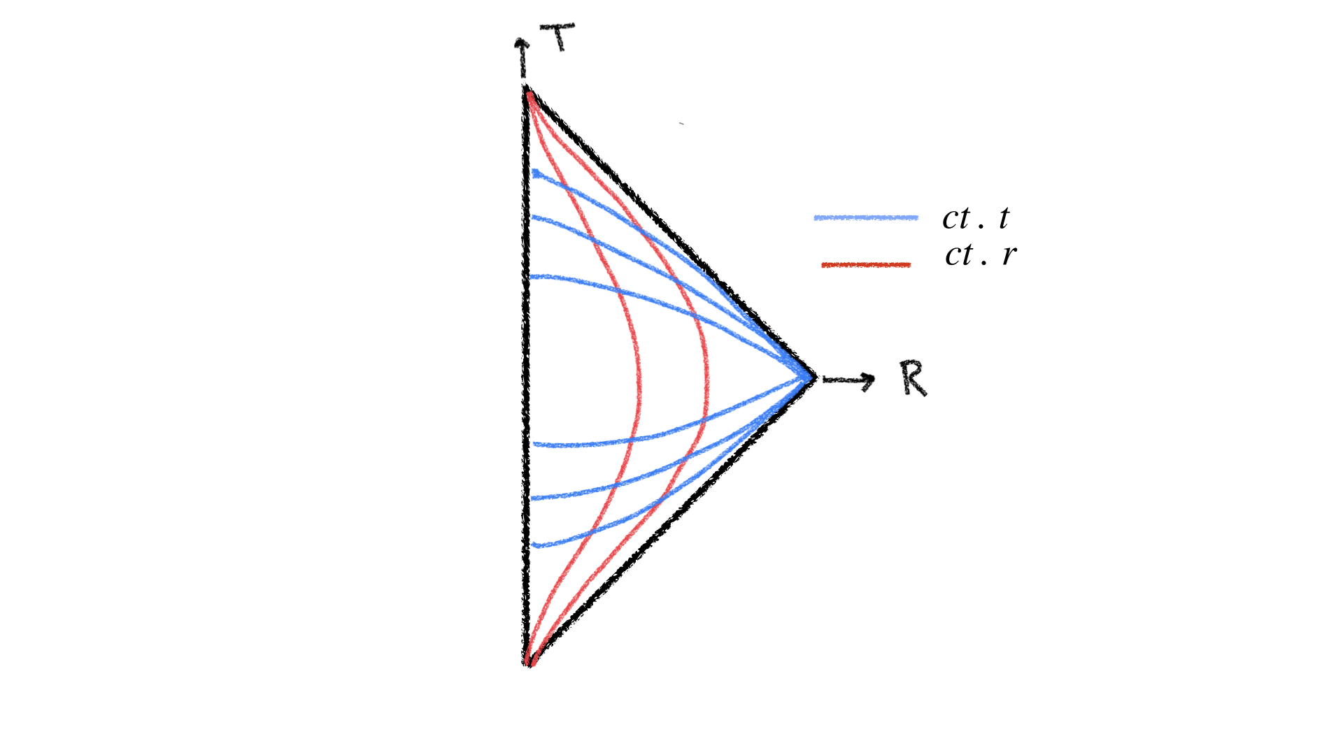
The asymptotic structure of (2.8) can be understood by introducing coordinates $(T,R)$ related to $(t,r)$ by

$$u=\tan U,\quad v=\tan V,\qquad T=U+V,\quad R=V-U,$$

(2.14)

in which case (2.8) reduces to

$$\begin{split}ds^{2}&=\Omega^{2}(T,R)\left(-dT^{2}+dR^{2}+2\sin^{2}R\gamma_{z\bar{z}}dzd\bar{z}\right),\\ \Omega^{-2}(T,R)&=4\cos^{2}\frac{1}{2}(T-R)\cos^{2}\frac{1}{2}(T+R).\end{split}$$

(2.15)

In the original coordinates, Minkowski space is covered by $r>0$, $-\infty<u<v<\infty$, therefore the ranges of the new coordinates are $-\frac{\pi}{2}<U<V<\frac{\pi}{2}$ and $0<R<\pi$. This is illustrated in figure 3.

It will be convenient to unfold this diagram to represent antipodal points on the spheres. Future null infinity ($\mathcal{I}^{+}$) is defined by taking $r\rightarrow\infty$ for fixed $u$, while past null infinity ($\mathcal{I}^{-}$) is reached by taking $r\rightarrow\infty$ for fixed $v$. In a free theory, massless particles follow lines of unit slope and cross points on the spheres at $\mathcal{I}^{\mp}$ at retarded times $v,u$. This is illustrated in figure 4. Massive particles never reach $\mathcal{I}^{\pm}$, but only past and future timelike infinities $i^{\mp}$ ($t\rightarrow\mp\infty$).

Asymptotically flat spacetimes have the same causal structure as Minkowski space at infinity. An asymptotically flat spacetime admits an expansion in powers of $r^{-1}$ around the Minkowski metric (2.12) near $\mathcal{I}^{+}$⁶⁶ 6 We are working in Bondi gauge defined by $\partial_{r}{\rm det}\left(\frac{g_{AB}}{r^{2}}\right)=0$ and $g_{rr}=g_{rA}=0$ where $A,B$ run over the transverse indices $z,\bar{z}.$ In these coordinates gravitational waves propagate radially outwards (equivalently, lines of constant $u,z,\bar{z}$ are null) and the wavefronts are spherical.

$$\begin{split}ds^{2}=&-du^{2}-2dudr+2r^{2}\gamma_{z\bar{z}}dzd\bar{z},\qquad\\ &+\frac{2m_{B}}{r}du^{2}+rC_{zz}dz^{2}+rC_{\bar{z}\bar{z}}d\bar{z}^{2}+2g_{uz}dudz+2g_{u\bar{z}}dud\bar{z}+\cdots.\end{split}$$

(2.16)

Solving the Einstein equations⁷⁷ 7 We set $\kappa=2$.

$$R_{\mu\nu}-\frac{1}{2}g_{\mu\nu}R=T^{M}_{\mu\nu}$$

(2.17)

order by order in a large-$r$ expansion⁸⁸ 8 The leading terms in the $uu$ and $uz$ components of the matter stress tensor are taken to be $\mathcal{O}(r^{-2})$. one finds [71]

$$g_{uz}=\frac{1}{2}D^{z}C_{zz}+\frac{1}{6r}C_{zz}D_{z}C^{zz}+\frac{2}{3r}N_{z}+\mathcal{O}(r^{-2}),$$

(2.18)

where $D_{z}$ is the covariant derivative associated with $\gamma_{z\bar{z}}$. Here $m_{B}$ and $N_{z}$ are the Bondi mass aspect and angular momentum aspect respectively, while

$$N_{zz}=\partial_{u}C_{zz}$$

(2.19)

is the outgoing news tensor. They are all functions of $(u,z,\bar{z})$.

$m_{B},C_{zz},N_{z}$ are not all independent. They are related by constraint equations.⁹⁹ 9 These are the components of (2.17) along the tangent to $\mathcal{I}^{+}.$ The $uu$ constraint gives [71]

$$\partial_{u}m_{B}=\frac{1}{4}D_{z}^{2}N^{zz}+\frac{1}{4}D_{\bar{z}}^{2}N^{\bar{z}\bar{z}}-\frac{1}{2}T_{uu}^{M(2)}-\frac{1}{4}N_{zz}N^{zz},$$

(2.20)

while the $uz$ constraint reduces to

$$\begin{split}\partial_{u}N_{z}=&\frac{1}{4}D_{z}\left(D_{z}^{2}C^{zz}-D_{\bar{z}}^{2}C^{\bar{z}\bar{z}}\right)-T_{uz}^{M(2)}+\partial_{z}m_{B}+\frac{1}{16}D_{z}\partial_{u}\left(C_{zz}C^{zz}\right)\\ &-\frac{1}{4}\left(N^{zz}D_{z}C_{zz}+N_{zz}D_{z}C^{zz}\right)-\frac{1}{4}D_{z}\left(C^{zz}N_{zz}-N^{zz}C_{zz}\right).\end{split}$$

(2.21)

We defined

$$T_{\mu\nu}^{M(2)}=\lim_{r\rightarrow\infty}r^{2}T_{\mu\nu}^{M}.$$

(2.22)

The square of $N_{zz}$ measures the energy carried by gravitational radiation. We learn from (2.20) that the Bondi mass (the integrated Bondi mass aspect over the sphere) is roughly speaking a measure of the net energy contained in spacetime excluding the parts carried off to infinity by null matter and gravitational waves: as energy is radiated away, the Bondi mass decreases. Similarly, the change in $N_{z}$ with retarded time (integrated over the sphere) measures the amount of angular momentum carried away to infinity by null matter and gravitational radiation.

The analogous equations near $\mathcal{I}^{-}$ can be found in [12].

The asymptotic symmetry group of (2.16) has beeen proposed to be the extended BMS⁺ group in [71]. This is generated by vector fields $\xi^{+}$ that preserve the asymptotic fall-off of (2.16) with $r$ namely

$$\mathcal{L}_{\xi^{+}}g_{ur}=\mathcal{O}(r^{-2}),\quad\mathcal{L}_{\xi^{+}}g_{uz}=\mathcal{O}(1),\quad\mathcal{L}_{\xi^{+}}g_{zz}=\mathcal{O}(r),\quad\mathcal{L}_{\xi^{+}}g_{uu}=\mathcal{O}(r^{-1}).$$

(2.23)

Here $\mathcal{L}_{\xi^{+}}$ is the Lie derivative with respect to $\xi^{+}$. Solving (2.23) order by order in a large-$r$ expansion, such vector fields are found to be of the form [71, 12]

$$\begin{split}\xi^{+}=&\left(1+\frac{u}{2r}\right)Y^{+z}\partial_{z}-\frac{u}{2r}D^{\bar{z}}D_{z}Y^{+z}\partial_{\bar{z}}-\frac{1}{2}(u+r)D_{z}Y^{+z}\partial_{r}+\frac{u}{2}D_{z}Y^{+z}\partial_{u}+c.c.\\ &+f^{+}\partial_{u}-\frac{1}{r}\left(D^{z}f^{+}\partial_{z}+D^{\bar{z}}f^{+}\partial_{\bar{z}}\right)+D^{z}D_{z}f^{+}\partial_{r}+\cdots,\end{split}$$

(2.24)

where $f^{+}(z,\bar{z})$ is an arbitrary function on $\mathcal{S}^{2}$ and $Y^{+}(z,\bar{z})$ is a conformal Killing vector on $\mathcal{S}^{2}$

$$\partial_{\bar{z}}Y^{+z}=0.$$

(2.25)

One easy way to see that (2.25) ought to hold is to notice that under Lorentz transformations,

$$\mathcal{L}_{Y^{+}}g_{\bar{z}\bar{z}}=2r^{2}\gamma_{z\bar{z}}\partial_{\bar{z}}Y^{+z}+\mathcal{O}(r).$$

(2.26)

Imposing that (2.23) are obeyed immediately leads to (2.25).

Globally, (2.25) admits six solutions

$$\begin{split}Y_{12}^{+z}&=-iz,\quad Y^{+z}_{13}=\frac{1}{2}(1+z^{2}),\quad Y^{+z}_{23}=\frac{i}{2}(1-z^{2}),\\ Y_{03}^{+z}&=-z,\quad Y^{+z}_{01}=\frac{1}{2}(1-z^{2}),\quad Y^{+z}_{02}=\frac{i}{2}(1+z^{2})\end{split}$$

(2.27)

corresponding to the three Lorentz rotations and three boosts (see appendix B). Locally, there are infinitely many solutions $Y^{+z}\propto z^{n}.$

For the remainder of this section, we restrict to the subgroup of asymptotic symmetries generated by (2.24) with $f=0$ which are known as superrotations [72].¹⁰¹⁰ 10 Conversely, supertranslations are the subset of symmetries (2.24) with $Y^{+}=0$ and $f\neq 0$. In this case, the vector fields (2.24) that map $\mathcal{I}^{+}$ to itself are

$$\xi^{+}\Big|_{\mathcal{I}^{+}}=Y^{+z}\partial_{z}+\frac{u}{2}D_{z}Y^{+z}\partial_{u}+c.c..$$

(2.28)

The infinitesimal BMS⁺ transformations (2.28) act on the metric components as follows

$$\begin{split}\delta_{Y^{+}}C_{zz}&=\frac{1}{2}\left(D_{z}Y^{+z}+D_{\bar{z}}Y^{+\bar{z}}\right)\left(u\partial_{u}-1\right)C_{zz}+\mathcal{L}_{Y^{+}}C_{zz}-uD_{z}^{3}Y^{+z},\\ \delta_{Y^{+}}N_{zz}&=\partial_{u}\delta_{Y^{+}}C_{zz}=\frac{u}{2}\left(D_{z}Y^{+z}+D_{\bar{z}}Y^{+\bar{z}}\right)\partial_{u}N_{zz}+\mathcal{L}_{Y^{+}}N_{zz}-D_{z}^{3}Y^{+z}.\end{split}$$

(2.29)

Upon quantization, (2.29) imply the existence of ‘‘charges’’¹¹¹¹ 11 We haven’t shown these are conserved yet; conservation will be implied by the subleading soft graviton theorem. under which an outgoing Fock state¹²¹² 12 The radiative data consists of the modes of $N_{zz}$ hence the action of $Q^{+}$ on the radiative part of $|{\rm out}\rangle$ is related to the commutator $[Q^{+},N_{zz}]$ [6]. transforms as

$$Q^{+}(Y^{+})|{\rm out}\rangle=i\delta_{Y^{+}}|{\rm out}\rangle,$$

(2.30)

where

$$Q^{+}(Y^{+})=Q^{+}_{H}+Q^{+}_{S}$$

(2.31)

and [72]

$$\begin{split}Q_{H}^{+}&=\frac{1}{4}\int_{\mathcal{I}^{+}}dud^{2}z\gamma_{z\bar{z}}\left(uD_{z}Y^{+z}N_{zz}N^{zz}-Y^{+z}D_{z}(C_{zz}N^{zz})-2Y^{+z}C_{zz}D_{z}N^{zz}+{\rm matter}\right)\\ &\hskip 370.0pt+c.c.,\\ Q_{S}^{+}&=-\frac{1}{2}\int_{\mathcal{I}^{+}}dud^{2}zD_{z}^{3}Y^{+z}uN^{z}_{\ \bar{z}}+c.c..\end{split}$$

(2.32)

We show in appendix A that (2.32) reproduce the symmetry action (2.29). Using the canonical commutation relations [73]

$$[N_{\bar{z}\bar{z}}(u,z,\bar{z}),C_{ww}(u^{\prime},w,\bar{w})]=2i\gamma_{z\bar{z}}\delta^{(2)}(z-w)\delta(u-u^{\prime}),$$

(2.33)

it then follows that for transformations parameterized by $Y^{+}=(Y^{+z},0)$ [12]

$$Q_{H}^{+}|{\rm out}\rangle=i\sum_{k\in{\rm out}}\left(\mathcal{L}_{Y^{+z_{k}}}-\frac{\omega_{k}}{2}D_{z_{k}}Y^{+z_{k}}\partial_{\omega_{k}}\right)|{\rm out}\rangle.$$

(2.34)

Similar formulas hold near $\mathcal{I}^{-}.$

An independent action of BMS⁺ and BMS^- on $\mathcal{I}^{+}$ and $\mathcal{I}^{-}$ leads to an ambiguity in defining scattering in AFS. In particular, upon specifying data at $\mathcal{I}^{+},$ the $S$-matrix provides a map between in and out states up to a BMS transformation.

A solution to this problem was proposed in [63] where it was shown that the gravitational scattering problem in AFS becomes well defined upon imposing the antipodal matching conditions

$$f(z,\bar{z})\Big|_{\mathcal{I}^{+}_{-}}=f(z,\bar{z})\Big|_{\mathcal{I}^{-}_{+}},\quad Y^{+}(z,\bar{z})\Big|_{\mathcal{I}^{+}_{-}}=Y^{-}(z,\bar{z})\Big|_{\mathcal{I}^{-}_{+}}.$$

(2.35)

Here, points on the sphere at $\mathcal{I}^{+}_{-}$ are antipodally related to points at $\mathcal{I}^{-}_{+}$, $(z,\bar{z})\Big|_{\mathcal{I}^{+}_{-}}=(-\frac{1}{\bar{z}},-\frac{1}{z})\Big|_{\mathcal{I}^{-}_{+}}$. Moreover, upon imposing the boundary condition¹³¹³ 13 Using the constraint (2.21) the superrotation charges can be put into the simpler form $Q^{+}(Y^{+})=\int d^{2}z\left(Y_{\bar{z}}^{+}N_{z}+Y_{z}^{+}N_{\bar{z}}\right)$ [10].

$$N_{z}(z,\bar{z})\Big|_{\mathcal{I}^{+}_{-}}=N_{z}(z,\bar{z})\Big|_{\mathcal{I}^{-}_{+}},$$

(2.36)

the charges at $\mathcal{I}^{-}_{+}$ and $\mathcal{I}^{+}_{-}$ obey

$$Q^{+}=Q^{-}.$$

(2.37)

The conservation of $Q$ implies the $\mathcal{S}$-matrix obeys the constraint

$$\langle{\rm out}|Q^{+}\mathcal{S}-\mathcal{S}Q^{-}|{\rm in}\rangle=0.$$

(2.38)

Using the split (2.31) into soft and hard parts, (2.38) is equivalent to

$$\langle{\rm out}|Q^{+}_{S}\mathcal{S}-\mathcal{S}Q^{-}_{S}|{\rm in}\rangle=-\langle{\rm out}|Q^{+}_{H}\mathcal{S}-\mathcal{S}Q^{-}_{H}|{\rm in}\rangle.$$

(2.39)

$Q_{S}$ is linear in the news and it can be shown to correspond to a mode of the graviton. In particular, one finds [12]

$$N_{\bar{z}\bar{z}}^{(1)}=\int_{-\infty}^{\infty}duuN_{\bar{z}\bar{z}}=\frac{i}{4\pi}\hat{\epsilon}_{\bar{z}\bar{z}}\lim_{\omega\rightarrow 0}(1+\omega\partial_{\omega})\left[a_{-}^{\rm out}(\omega\hat{x})-a_{+}^{{\rm out}\dagger}(\omega\hat{x})\right]$$

(2.40)

and hence $Q_{S}$ picks out a particular subleading¹⁴¹⁴ 14 $1+\omega\partial_{\omega}$ projects out the leading soft pole. soft graviton mode.

For simplicity we now restrict to the case when all asymptotic particles but the soft insertion are scalars. Using the subleading soft relation (2.2), the LHS of (2.39) reduces to [12]

$$\begin{split}\langle{\rm out}|Q^{+}_{S}\mathcal{S}-\mathcal{S}Q^{-}_{S}|{\rm in}\rangle&=-\frac{i}{4\pi}\int d^{2}zD_{z}^{3}Y^{z}\hat{\epsilon}_{\bar{z}\bar{z}}S^{(1)-}\langle{\rm out}|\mathcal{S}|{\rm in}\rangle\\ &=-i\sum_{k\in{\rm in,out}}\left(Y^{z_{k}}\partial_{z_{k}}-\frac{\omega_{k}}{2}D_{z_{k}}Y^{z_{k}}\partial_{\omega_{k}}\right)\langle{\rm out}|\mathcal{S}|{\rm in}\rangle.\end{split}$$

(2.41)

In the second line, we integrated by parts and used the parameterizations of momenta

$$q(\omega,z,\bar{z})=\omega\hat{q}(z,\bar{z})=\frac{\omega}{1+z\bar{z}}\left(1+z\bar{z},z+\bar{z},-i(z-\bar{z}),1-z\bar{z}\right)$$

(2.42)

for which the subleading soft factor for a negative helicity graviton becomes

$$S^{(1)-}=\sum_{k}\left(\frac{(z-z_{k})(1+z\bar{z}_{k})}{(\bar{z}_{k}-\bar{z})(1+z_{k}\bar{z}_{k})}\omega_{k}\partial_{\omega_{k}}+\frac{(z-z_{k})^{2}}{\bar{z}_{k}-\bar{z}}\partial_{z_{k}}\right).$$

(2.43)

The RHS of (2.41) coincides with the action (2.34) of the hard charge $Q_{H}$ on scalar asymptotic states. We conclude the tree-level subleading soft theorem implies the conservation of the charges (2.31), hence the enhancement of Lorentz symmetry to Virasoro.

(2.41) also points to another remarkable feature of gravity in AFS: the existence of a subleading soft graviton mode whose insertions in the quantum gravity $\mathcal{S}$-matrix behaves like the stress tensor of a 2D CFT. To see this, we simply set

$$Y^{z_{k}}=\frac{1}{z-z_{k}}$$

(2.44)

in (2.41). Upon defining¹⁵¹⁵ 15 Note that this operator is directly related to the soft charges $Q_{S}^{\pm}$ evaluated at $Y^{w}=\frac{1}{z-w}$.

$$T_{zz}\equiv i\int d^{2}w\frac{1}{z-w}D_{w}^{2}D^{\bar{w}}N_{\bar{w}\bar{w}}^{(1)},$$

(2.45)

(2.41) reduces to

$$\langle T_{zz}\mathcal{O}_{1}...\mathcal{O}_{n}\rangle=\sum_{k=1}^{n}\left[\frac{\hat{h}_{k}}{(z-z_{k})^{2}}+\frac{\Gamma_{\ z_{k}z_{k}}^{z_{k}}}{z-z_{k}}\hat{h}_{k}+\frac{1}{z-z_{k}}\partial_{z_{k}}\right]\langle\mathcal{O}_{1}...\mathcal{O}_{n}\rangle.$$

(2.46)

This is the Ward identity of a stress tensor in a conformal field theory on a curved background [74]. Note however that the weight¹⁶¹⁶ 16 For external states of spin $s_{k}$, the weights generalize to $\hat{h}_{k}=\frac{s_{k}-\omega_{k}\partial_{\omega_{k}}}{2}$ and (2.46) gets corrected by a spin connection term, see [13] for the general formula. $\hat{h}_{k}=-\frac{1}{2}\omega_{k}\partial_{\omega_{k}}$ is a differential operator which acts non-diagonally on $S$-matrix elements in a basis of momentum eigenstates. In the next section we will introduce a new basis of asymptotic states which diagonalize the action of $\hat{h}_{k}$. The scattering problem in AFS will be then reformulated in terms of an observable living on the celestial sphere: the celestial amplitude.

Scalar conformal primary wavefunctions are solutions to the wave equation

$$\left(\nabla^{2}-m^{2}\right)\Psi=0,$$

(3.1)

which are “highest weight” with respect to the Lorentz SO$(1,3)$. We start by identifying the associated highest weight states, then impose they are solutions to (3.1). A representation of the Lorentz generators is

$$J^{\mu\nu}=L^{\mu\nu}+S^{\mu\nu},$$

(3.2)

where

$$L^{\mu\nu}=-\left(x^{\mu}\partial^{\nu}-x^{\nu}\partial^{\mu}\right)$$

(3.3)

is the orbital angular momentum generator and $S^{\mu\nu}$ is the spin generator. For simplicity, we focus on scalars in which case $S^{\mu\nu}=0.$

(3.3) consist of rotations

$$J_{1}=-(x^{2}\partial_{x^{3}}-x^{3}\partial_{x^{2}}),~~~J_{2}=x^{1}\partial_{x^{3}}-x^{3}\partial_{x^{1}},~~~J_{3}=-(x^{1}\partial_{x^{2}}-x^{2}\partial_{x^{1}})$$

(3.4)

and boosts

$$\begin{split}K_{1}=-(x^{0}\partial_{x^{1}}+x^{1}\partial_{x^{0}}),~~~K_{2}=-(x^{0}\partial_{x^{2}}+x^{2}\partial_{x^{0}}),~~~K_{3}=-(x^{0}\partial_{x^{3}}+x^{3}\partial_{x^{0}}).\end{split}$$

(3.5)

These generators obey the standard Lorentz algebra

$$\begin{split}[J_{i},J_{j}]&=\epsilon_{ijk}J_{k},\\ [K_{i},K_{j}]&=-\epsilon_{ijk}J_{k},\\ [J_{i},K_{j}]&=\epsilon_{ijk}K_{k},\end{split}$$

(3.6)

while the linear combinations (B.1) of (3.4), (3.5) in appendix B obey the SL$(2,\mathbb{C})$ commutation relations

$$[L_{m},L_{n}]=(m-n)L_{m+n},\quad[\bar{L}_{m},\bar{L}_{n}]=(m-n)\bar{L}_{m+n}.$$

(3.7)

We now notice that

$$\Psi_{\Delta}\propto\frac{1}{(x^{0}+x^{3})^{\Delta}}$$

(3.8)

obeys

$$(L_{0}+\bar{L}_{0})\Psi_{\Delta}=\Delta\Psi_{\Delta},\quad(L_{0}-\bar{L}_{0})\Psi_{\Delta}=0$$

(3.9)

as well as

$$L_{1}\Psi_{\Delta}=\bar{L}_{1}\Psi_{\Delta}=0.$$

(3.10)

In other words, (3.8) diagonalizes boosts in the $x^{3}$ direction and obeys the highest weight condition (3.10).

One could repeat this analysis starting with a set of rotated bulk Lorentz generators,

$$J_{i}^{\prime}=R_{ij}J_{j},\quad K_{i}^{\prime}=R_{ij}K_{j},$$

(3.11)

where

$$R=\left(\begin{matrix}\cos\hat{\varphi}\cos\hat{\theta}&&\sin\hat{\varphi}\cos\hat{\theta}&&-\sin\hat{\theta}\\ -\sin\hat{\varphi}&&\cos\hat{\varphi}&&0\\ \cos\hat{\varphi}\sin\hat{\theta}&&\sin\hat{\varphi}\sin\hat{\theta}&&\cos\hat{\theta}\end{matrix}\right)\equiv\left(\begin{matrix}\hat{n}_{1}\\ \hat{n}_{2}\\ \hat{n}_{3}\end{matrix}\right).$$

Multiplication by an arbitrary function $f$ of the Lorentz invariant $x^{2}$ will preserve both the eigenvalue and highest weight conditions (3.9), (3.10), hence in general, a highest weight solution diagonal with respect to $K_{3}^{\prime}$ will be¹⁷¹⁷ 17 $(\hat{\theta},\hat{\varphi})$ are related to $z,\bar{z}$ via the stereographic projection.

$$\Psi_{\Delta}(\hat{q};x)=\frac{f(x^{2})}{(\hat{q}\cdot x)^{\Delta}},\quad\hat{q}=\left(1,\hat{n}_{3}\right)=\hat{q}(z,\bar{z}),$$

(3.12)

with $\hat{q}(z,\bar{z})$ in (2.42).

Finally, we require that (3.12) obeys the wave equation. Plugging (3.12) into (3.1), we find the following differential equation for $f$ [14]

$$4x^{2}f^{\prime\prime}(x^{2})-4(\Delta-2)f^{\prime}(x^{2})-m^{2}f(x^{2})=0.$$

(3.13)

The solutions to (3.13) are linear combination of Bessel functions (of first kind)

$$f(x^{2})=\left(\sqrt{-x^{2}}\right)^{\Delta-1}\left[c_{1}I_{\Delta-1}(m\sqrt{x^{2}})+c_{2}I_{-\Delta+1}(m\sqrt{x^{2}})\right],$$

(3.14)

where $c_{1},c_{2}$ are ($\Delta$-dependent) constants. Imposing that (3.14) decays to $0$ as $x^{2}\rightarrow\infty$ picks out the linear combination proportional to the Bessel function of second kind

$$f(x^{2})\propto\left(\sqrt{-x^{2}}\right)^{\Delta-1}K_{\Delta-1}(m\sqrt{x^{2}}).$$

(3.15)

We conclude that up to normalization, the massive conformal primary wavefunctions take the form¹⁸¹⁸ 18 An $i\epsilon$ prescription distinguishes between in and out states [14].

$$\Psi_{\Delta}(\hat{q};x)\propto\frac{\left(\sqrt{-x^{2}}\right)^{\Delta-1}}{(\hat{q}\cdot x)^{\Delta}}K_{\Delta-1}(m\sqrt{x^{2}}).$$

(3.16)

Under Lorentz transformations, both $\hat{q}$ and $x$ transform linearly

$$\begin{split}\hat{q}^{\mu}(z^{\prime},\bar{z}^{\prime})&=\left|\frac{\partial\vec{z}^{\prime}}{\partial\vec{z}}\right|^{1/2}\Lambda^{\mu}_{\ \nu}\hat{q}^{\nu}(z,\bar{z}),\\ x^{\mu^{\prime}}&=\Lambda^{\mu}_{\ \nu}x^{\nu}\end{split}$$

(3.17)

hence (3.16) obeys

$$\Psi_{\Delta}(\Lambda^{\mu}_{\ \nu}x;\vec{z}^{\prime}(\vec{z}))=\Big|\frac{\partial\vec{z}^{\prime}}{\partial\vec{z}}\Big|^{-\Delta/2}\Psi_{\Delta}(x;\vec{z}).$$

(3.18)

In the next section we give an alternate derivation of (3.16) which will lead to a representation of (3.16) as Fourier transforms of $AdS_{3}$ bulk-to-boundary propagators.

The conformal compactification of Minkowski space in section 2.2 obscures one aspect of scattering in AFS: all massive particles enter (exit) spacetime at a point, $i^{-}(i^{+})$, so how are we supposed to distingush between different asymptotics? The key is to resolve past and future timelike infinities by introducing the new coordinates [75, 76]

$$\begin{split}t^{2}-r^{2}&=\tau^{2},\\ \rho\tau&=r.\end{split}$$

(3.19)

In $(\tau,\rho,z,\bar{z})$ coordinates, (2.8) becomes

$$ds^{2}=-d\tau^{2}+\tau^{2}\left(\frac{d\rho^{2}}{1+\rho^{2}}+2\rho^{2}\gamma_{z\bar{z}}dzd\bar{z}\right)=-d\tau^{2}+\tau^{2}ds_{\mathbb{H}_{3}}.$$

(3.20)

We learn that slices of constant $\tau$ correspond to hyperboloids of radius $\tau$, while $\rho=\dfrac{r}{t}\left(1-\dfrac{r^{2}}{t^{2}}\right)^{-1/2}$ is constant whenever $r/t$ is constant. Note also that since $t=\tau\sqrt{1+\rho^{2}}$, the limit $\tau\rightarrow\infty$ corresponds to $t\rightarrow\infty$ for fixed $(\rho,z,\bar{z})$. We illustrate the foliations of the past and future light-cones (also known as Milne wedges) with $\mathbb{H}_{3}$ slices in figure 5.

Parameterizing the trajectory of a massive particle of constant momentum $\vec{p}$ and energy $E$ by

$$\vec{r}=\vec{r}_{0}+\frac{t}{E}\vec{p},$$

(3.21)

we find that as $t\rightarrow\infty$,

$$\rho\rightarrow\frac{|\vec{p}|}{m},\quad\frac{\vec{r}}{r}\rightarrow\frac{\vec{p}}{p}.$$

(3.22)

Hence at late times, the massive particle asymptotes to fixed $(\rho,z,\bar{z})$, or equivalently a point on the unit hyperboloid at $i^{+}$. Similarily, the Rindler wedges can be foliated with $dS_{3}$ slices. This slicing is easily obtained by letting

$$\tau=i\widetilde{\tau},\quad\rho=-i\widetilde{\rho}$$

(3.23)

in (3.20) in which case

$$ds^{2}=d\widetilde{\tau}^{2}+\widetilde{\tau}^{2}\left(\frac{d\widetilde{\rho}^{2}}{1-\widetilde{\rho}^{2}}+2\widetilde{\rho}^{2}\gamma_{z\bar{z}}dzd\bar{z}\right).$$

(3.24)

This $dS_{3}$ slicing won’t be discussed further herein, but see [77] for an analysis of associated conformal primary solutions.

The proper, orthocronous Lorentz group acts as the group of isometries on the $\mathbb{H}_{3}$ slices for $t>0$. To find solutions to (3.1) that preserve slices of constant $\tau$ it is convenient to express $\nabla^{2}$ with respect to the coordinates in (3.20) .

References

- [1] J. M. Maldacena, “The Large N limit of superconformal field theories and supergravity,” Int. J. Theor. Phys. 38 (1999) 1113–1133, arXiv:hep-th/9711200 [hep-th]. [Adv. Theor. Math. Phys.2,231(1998)].
- [2] O. Aharony, S. S. Gubser, J. M. Maldacena, H. Ooguri, and Y. Oz, “Large N field theories, string theory and gravity,” Phys. Rept. 323 (2000) 183–386, arXiv:hep-th/9905111 [hep-th].
- [3] S. Ryu and T. Takayanagi, “Holographic derivation of entanglement entropy from AdS/CFT,” Phys. Rev. Lett. 96 (2006) 181602, arXiv:hep-th/0603001.
- [4] L. Susskind, “The World as a hologram,” J. Math. Phys. 36 (1995) 6377–6396, arXiv:hep-th/9409089 [hep-th].
- [5] R. Bousso, “The Holographic principle,” Rev. Mod. Phys. 74 (2002) 825–874, arXiv:hep-th/0203101.
- [6] T. He, V. Lysov, P. Mitra, and A. Strominger, “BMS supertranslations and Weinberg’s soft graviton theorem,” JHEP 05 (2015) 151, arXiv:1401.7026 [hep-th].
- [7] T. He, P. Mitra, A. P. Porfyriadis, and A. Strominger, “New Symmetries of Massless QED,” JHEP 10 (2014) 112, arXiv:1407.3789 [hep-th].
- [8] A. Strominger and A. Zhiboedov, “Gravitational Memory, BMS Supertranslations and Soft Theorems,” JHEP 01 (2016) 086, arXiv:1411.5745 [hep-th].
- [9] S. Pasterski, “Asymptotic Symmetries and Electromagnetic Memory,” JHEP 09 (2017) 154, arXiv:1505.00716 [hep-th].
- [10] A. Strominger, “Lectures on the Infrared Structure of Gravity and Gauge Theory,” arXiv:1703.05448 [hep-th].
- [11] S. Pasterski, S.-H. Shao, and A. Strominger, “Flat Space Amplitudes and Conformal Symmetry of the Celestial Sphere,” Phys. Rev. D96 no. 6, (2017) 065026, arXiv:1701.00049 [hep-th].
- [12] D. Kapec, V. Lysov, S. Pasterski, and A. Strominger, “Semiclassical Virasoro symmetry of the quantum gravity -matrix,” JHEP 08 (2014) 058, arXiv:1406.3312 [hep-th].
- [13] D. Kapec, P. Mitra, A.-M. Raclariu, and A. Strominger, “2D Stress Tensor for 4D Gravity,” Phys. Rev. Lett. 119 no. 12, (2017) 121601, arXiv:1609.00282 [hep-th].
- [14] S. Pasterski and S.-H. Shao, “Conformal basis for flat space amplitudes,” Phys. Rev. D96 no. 6, (2017) 065022, arXiv:1705.01027 [hep-th].
- [15] H. T. Lam and S.-H. Shao, “Conformal Basis, Optical Theorem, and the Bulk Point Singularity,” Phys. Rev. D98 no. 2, (2018) 025020, arXiv:1711.06138 [hep-th].
- [16] S. Stieberger and T. R. Taylor, “Symmetries of Celestial Amplitudes,” Phys. Lett. B793 (2019) 141–143, arXiv:1812.01080 [hep-th].
- [17] Y. T. A. Law and M. Zlotnikov, “Poincare constraints on celestial amplitudes,” JHEP 03 (2020) 085, arXiv:1910.04356 [hep-th].
- [18] M. Pate, A.-M. Raclariu, A. Strominger, and E. Y. Yuan, “Celestial Operator Products of Gluons and Gravitons,” arXiv:1910.07424 [hep-th].
- [19] A. Guevara, E. Himwich, M. Pate, and A. Strominger, “Holographic Symmetry Algebras for Gauge Theory and Gravity,” arXiv:2103.03961 [hep-th].
- [20] A. Strominger, “w(1+infinity) and the Celestial Sphere,” arXiv:2105.14346 [hep-th].
- [21] S. Pasterski, S.-H. Shao, and A. Strominger, “Gluon Amplitudes as 2d Conformal Correlators,” Phys. Rev. D96 no. 8, (2017) 085006, arXiv:1706.03917 [hep-th].
- [22] A. Schreiber, A. Volovich, and M. Zlotnikov, “Tree-level gluon amplitudes on the celestial sphere,” Phys. Lett. B781 (2018) 349–357, arXiv:1711.08435 [hep-th].
- [23] S. Stieberger and T. R. Taylor, “Strings on Celestial Sphere,” Nucl. Phys. B935 (2018) 388–411, arXiv:1806.05688 [hep-th].
- [24] N. Kalyanapuram, “Gauge and Gravity Amplitudes on the Celestial Sphere,” Phys. Rev. D 103 no. 8, (2021) 085015, arXiv:2012.04579 [hep-th].
- [25] A. Brandhuber, G. R. Brown, J. Gowdy, B. Spence, and G. Travaglini, “Celestial Superamplitudes,” arXiv:2105.10263 [hep-th].
- [26] H. Jiang, “Celestial superamplitude in SYM theory,” arXiv:2105.10269 [hep-th].
- [27] Y. Hu, L. Ren, A. Y. Srikant, and A. Volovich, “Celestial Dual Superconformal Symmetry, MHV Amplitudes and Differential Equations,” arXiv:2106.16111 [hep-th].
- [28] N. Banerjee, S. Banerjee, S. Atul Bhatkar, and S. Jain, “Conformal Structure of Massless Scalar Amplitudes Beyond Tree level,” JHEP 04 (2018) 039, arXiv:1711.06690 [hep-th].
- [29] H. A. González, A. Puhm, and F. Rojas, “Loop corrections to celestial amplitudes,” Phys. Rev. D 102 no. 12, (2020) 126027, arXiv:2009.07290 [hep-th].
- [30] S. Albayrak, C. Chowdhury, and S. Kharel, “Loop celestial amplitudes for gauge theory and gravity,” Phys. Rev. D 102 (Dec, 2020) 126020. https://link.aps.org/doi/10.1103/PhysRevD.102.126020.
- [31] T. Adamo, L. Mason, and A. Sharma, “Celestial amplitudes and conformal soft theorems,” Class. Quant. Grav. 36 no. 20, (2019) 205018, arXiv:1905.09224 [hep-th].
- [32] E. Casali and A. Puhm, “Double Copy for Celestial Amplitudes,” Phys. Rev. Lett. 126 no. 10, (2021) 101602, arXiv:2007.15027 [hep-th].
- [33] E. Casali and A. Sharma, “Celestial double copy from the worldsheet,” JHEP 05 (2021) 157, arXiv:2011.10052 [hep-th].
- [34] M. Campiglia and S. Nagy, “A double copy for asymptotic symmetries in the self-dual sector,” JHEP 03 (2021) 262, arXiv:2102.01680 [hep-th].
- [35] J. Distler, R. Flauger, and B. Horn, “Double-soft graviton amplitudes and the extended BMS charge algebra,” JHEP 08 (2019) 021, arXiv:1808.09965 [hep-th].
- [36] S. Banerjee, “Null Infinity and Unitary Representation of The Poincare Group,” JHEP 01 (2019) 205, arXiv:1801.10171 [hep-th].
- [37] S. Banerjee, P. Pandey, and P. Paul, “Conformal properties of soft-operators - 1 : Use of null-states,” arXiv:1902.02309 [hep-th].
- [38] A. Puhm, “Conformally Soft Theorem in Gravity,” arXiv:1905.09799 [hep-th].
- [39] W. Fan, A. Fotopoulos, S. Stieberger, and T. R. Taylor, “On Sugawara construction on Celestial Sphere,” JHEP 09 (2020) 139, arXiv:2005.10666 [hep-th].
- [40] A. Fotopoulos, S. Stieberger, T. R. Taylor, and B. Zhu, “Extended BMS Algebra of Celestial CFT,” arXiv:1912.10973 [hep-th].
- [41] Y. T. A. Law and M. Zlotnikov, “Massive Spinning Bosons on the Celestial Sphere,” JHEP 06 (2020) 079, arXiv:2004.04309 [hep-th].
- [42] S. Ebert, A. Sharma, and D. Wang, “Descendants in celestial CFT and emergent multi-collinear factorization,” JHEP 03 (2021) 030, arXiv:2009.07881 [hep-th].
- [43] S. Banerjee and S. Ghosh, “MHV Gluon Scattering Amplitudes from Celestial Current Algebras,” arXiv:2011.00017 [hep-th].
- [44] S. Banerjee, S. Ghosh, and R. Gonzo, “BMS symmetry of celestial OPE,” JHEP 04 (2020) 130, arXiv:2002.00975 [hep-th].
- [45] S. Banerjee, S. Ghosh, and S. Satyam Samal, “Subsubleading soft graviton symmetry and MHV graviton scattering amplitudes,” arXiv:2104.02546 [hep-th].
- [46] S. Pasterski, A. Puhm, and E. Trevisani, “Revisiting the Conformally Soft Sector with Celestial Diamonds,” arXiv:2105.09792 [hep-th].
- [47] S. Pasterski, A. Puhm, and E. Trevisani, “Celestial Diamonds: Conformal Multiplets in Celestial CFT,” arXiv:2105.03516 [hep-th].
- [48] N. Arkani-Hamed, M. Pate, A.-M. Raclariu, and A. Strominger, “Celestial Amplitudes from UV to IR,” arXiv:2012.04208 [hep-th].
- [49] C.-M. Chang, Y.-t. Huang, Z.-X. Huang, and W. Li, “Bulk locality from the celestial amplitude,” arXiv:2106.11948 [hep-th].
- [50] D. Nandan, A. Schreiber, A. Volovich, and M. Zlotnikov, “Celestial Amplitudes: Conformal Partial Waves and Soft Limits,” JHEP 10 (2019) 018, arXiv:1904.10940 [hep-th].
- [51] Y. T. A. Law and M. Zlotnikov, “Relativistic partial waves for celestial amplitudes,” JHEP 11 (2020) 149, arXiv:2008.02331 [hep-th].
- [52] W. Fan, A. Fotopoulos, S. Stieberger, T. R. Taylor, and B. Zhu, “Conformal blocks from celestial gluon amplitudes,” JHEP 05 (2021) 170, arXiv:2103.04420 [hep-th].
- [53] A. Atanasov, W. Melton, A.-M. Raclariu, and A. Strominger, “Conformal Block Expansion in Celestial CFT,” arXiv:2104.13432 [hep-th].
- [54] S. Choi and R. Akhoury, “Magnetic soft charges, dual supertranslations, and ’t Hooft line dressings,” Phys. Rev. D 102 no. 2, (2020) 025001, arXiv:1912.02224 [hep-th].
- [55] A. Laddha, S. G. Prabhu, S. Raju, and P. Shrivastava, “The Holographic Nature of Null Infinity,” SciPost Phys. 10 (2021) 041, arXiv:2002.02448 [hep-th].
- [56] E. Hijano and D. Neuenfeld, “Soft photon theorems from CFT Ward identites in the flat limit of AdS/CFT,” JHEP 11 (2020) 009, arXiv:2005.03667 [hep-th].
- [57] E. Himwich, S. A. Narayanan, M. Pate, N. Paul, and A. Strominger, “The Soft -Matrix in Gravity,” JHEP 09 (2020) 129, arXiv:2005.13433 [hep-th].
- [58] H. Hirai and S. Sugishita, “IR finite S-matrix by gauge invariant dressed states,” JHEP 02 (2021) 025, arXiv:2009.11716 [hep-th].
- [59] L. Freidel, J. Kowalski-Glikman, R. G. Leigh, and D. Minic, “Quantum Gravity Phenomenology in the Infrared,” arXiv:2104.00802 [gr-qc].
- [60] H. A. González and F. Rojas, “The structure of IR divergences in celestial gluon amplitudes,” arXiv:2104.12979 [hep-th].
- [61] K. Nguyen and J. Salzer, “Celestial IR divergences and the effective action of supertranslation modes,” arXiv:2105.10526 [hep-th].
- [62] L. Lippstreu, “Zwanziger’s pairwise little group on the celestial sphere,” arXiv:2106.00084 [hep-th].
- [63] A. Strominger, “On BMS Invariance of Gravitational Scattering,” JHEP 07 (2014) 152, arXiv:1312.2229 [hep-th].
- [64] T. He, P. Mitra, and A. Strominger, “2D Kac-Moody Symmetry of 4D Yang-Mills Theory,” JHEP 10 (2016) 137, arXiv:1503.02663 [hep-th].
- [65] F. E. Low, “Bremsstrahlung of very low-energy quanta in elementary particle collisions,” Phys. Rev. 110 (1958) 974–977.
- [66] S. Weinberg, “Infrared photons and gravitons,” Phys. Rev. 140 (Oct, 1965) B516–B524. https://link.aps.org/doi/10.1103/PhysRev.140.B516.
- [67] F. Cachazo and A. Strominger, “Evidence for a New Soft Graviton Theorem,” arXiv:1404.4091 [hep-th].
- [68] S. He, Y.-t. Huang, and C. Wen, “Loop Corrections to Soft Theorems in Gauge Theories and Gravity,” JHEP 12 (2014) 115, arXiv:1405.1410 [hep-th].
- [69] H. Elvang, C. R. T. Jones, and S. G. Naculich, “Soft Photon and Graviton Theorems in Effective Field Theory,” Phys. Rev. Lett. 118 no. 23, (2017) 231601, arXiv:1611.07534 [hep-th].
- [70] A. Laddha and P. Mitra, “Asymptotic Symmetries and Subleading Soft Photon Theorem in Effective Field Theories,” JHEP 05 (2018) 132, arXiv:1709.03850 [hep-th].
- [71] G. Barnich and C. Troessaert, “BMS charge algebra,” JHEP 12 (2011) 105, arXiv:1106.0213 [hep-th].
- [72] G. Barnich and C. Troessaert, “Supertranslations call for superrotations,” PoS CNCFG2010 (2010) 010, arXiv:1102.4632 [gr-qc]. [Ann. U. Craiova Phys.21,S11(2011)].
- [73] A. Ashtekar, Asymptotic quantization: based on 1984 Naples lectures. 1987.
- [74] T. Eguchi and H. Ooguri, “Conformal and current algebras on a general riemann surface,” Nuclear Physics B 282 (1987) 308–328. https://www.sciencedirect.com/science/article/pii/0550321387906869.
- [75] J. de Boer and S. N. Solodukhin, “A holographic reduction of minkowski spacetime,” Nuclear Physics B 665 (2003) 545 – 593. http://www.sciencedirect.com/science/article/pii/S0550321303004942.
- [76] M. Campiglia and A. Laddha, “Asymptotic symmetries of QED and Weinberg’s soft photon theorem,” JHEP 07 (2015) 115, arXiv:1505.05346 [hep-th].
- [77] C. Liu and D. A. Lowe, “Conformal Wave Expansions for Flat Space Amplitudes,” arXiv:2105.01026 [hep-th].
- [78] A. Atanasov, A. Ball, W. Melton, A.-M. Raclariu, and A. Strominger, “ Scattering and the Celestial Torus,” arXiv:2101.09591 [hep-th].
- [79] E. Witten, “Anti-de Sitter space and holography,” Adv. Theor. Math. Phys. 2 (1998) 253–291, arXiv:hep-th/9802150 [hep-th].
- [80] D. Kutasov and N. Seiberg, “More comments on string theory on AdS(3),” JHEP 04 (1999) 008, arXiv:hep-th/9903219.
- [81] L. Donnay, A. Puhm, and A. Strominger, “Conformally Soft Photons and Gravitons,” JHEP 01 (2019) 184, arXiv:1810.05219 [hep-th].
- [82] S. A. Narayanan, “Massive Celestial Fermions,” JHEP 12 (2020) 074, arXiv:2009.03883 [hep-th].
- [83] L. Iacobacci and W. Mück, “Conformal Primary Basis for Dirac Spinors,” Phys. Rev. D 102 no. 10, (2020) 106025, arXiv:2009.02938 [hep-th].
- [84] S. Pasterski and A. Puhm, “Shifting Spin on the Celestial Sphere,” arXiv:2012.15694 [hep-th].
- [85] M. Pate, A.-M. Raclariu, and A. Strominger, “Conformally Soft Theorem in Gauge Theory,” Phys. Rev. D100 no. 8, (2019) 085017, arXiv:1904.10831 [hep-th].
- [86] J. D. Qualls, “Lectures on Conformal Field Theory,” arXiv:1511.04074 [hep-th].
- [87] A. Guevara, “Notes on Conformal Soft Theorems and Recursion Relations in Gravity,” arXiv:1906.07810 [hep-th].
- [88] L. Donnay, S. Pasterski, and A. Puhm, “Asymptotic Symmetries and Celestial CFT,” JHEP 09 (2020) 176, arXiv:2005.08990 [hep-th].