Exponential convergence of perfectly matched layers for scattering problems with periodic surfaces
Ruming Zhang
Thanks: Institute of Applied and Numerical mathematics, Karlsruhe Institute of Technology, Karlsruhe, Germany
; ruming.zhang@kit.edu.
Abstract
The main task in this paper is to prove that the perfectly matched layers (PML) method converges exponentially with respect to the PML parameter for scattering problems with periodic surfaces. In [6], a linear convergence is proved for the PML method for scattering problems with rough surfaces. At the end of that paper, three important questions were asked, and the third question is if exponential convergence holds locally. In our paper, we answer this question for a special case, when the rough surface is actually periodic. The result can also be easily extended to locally perturbed periodic surfaces or layers. Due to technical reasons, we have to exclude all the wavenumbers which are half integers. The main idea of the proof is to apply the Floquet-Bloch transform to rewrite the problem as an equivalent family of quasi-periodic problems, and then study the analytic extension of the quasi-periodic problems with respect to the Floquet-Bloch parameters. Then the Cauchy integral formula is applied to avoid linear convergent points. Finally the exponential convergence is proved from the inverse Floquet-Bloch transform. Numerical results are also presented at the end of this paper.
The PML method has been widely applied to the simulation of wave propagations in unbounded domains since it was invented in [2]. The main idea for the PML method is to add an artificial absorbing layer outside the scatterers, where there is almost no reflection. The problem is then approximated by the truncation with a proper boundary condition. To guarantee that the PML method works, it is of essential importance to study the convergence of the solution with respect to the PML parameters.
This paper studies the convergence of the PML method for acoustic scattering problems with periodic surfaces in two dimensional spaces. This paper is motivated by the open questions at the end of [6]. Although a linear convergence has been proved for rough surfaces in that paper, exponential convergence was shown for an extreme case when the surface is flat. The authors conjectured that the exponential convergence held locally also for nonflat surfaces. In this paper, we try to answer this question for periodic surfaces, using techniques introduced in [7]. First, we introduce the setting of this problem as well as some important notations and spaces.
Suppose is a surface defined by a -periodic Lipschitz continuous function , and is the unbounded periodic domain above :
For simplicity, we only consider the problem described by the following model:
(1)
where is a compactly supported source term.
Let be a number such that
Let be a straight line lying above and let the periodic strip between and be denoted by . Then . Thus satisfies the homogeneous Helmholtz equation when .
To guarantee that the solution propagates upwards, we also require that satisfies the following radiation condition (see [5]):
where is the Fourier transform of and has non-negative real and imaginary parts. This radiation condition defines the following DtN map on :
From [5], is a bounded operator from to . Thus satisfies the following boundary condition:
(2)
Now the problem is formulated in the periodic domain with finite height by (1)-(2). The weak formulation is straight forward, i.e., to find such that
(3)
holds for any compactly supported , where
From [5] it is known that the problem (3) is uniquely solvable in . For unique solvability in the weighted Sobolev space () we refer to [4].
We apply the Floquet-Bloch transform to (3), and the problem is written as a family of quasi-periodic problems, and the original solution is then written as the inverse Floquet-Bloch transform of quasi-periodic problems, which is an integral on an interval with respect to the Floquet-Bloch parameters. The quasi-periodic problems depend piecewise smoothly on the Floquet-Bloch parameters, with only one or two square root singularities (later called “cutoff values”). At the cutoff values, only linear convergence are proved for the PML method. For parameters away from those points, exponential convergence is proved. For details we refer to [7, 6, 10]. To the best of the author’s knowledge, the exponential convergence for rough surfaces (including periodic surfaces) is only proved for complex valued wavenumbers, for details we refer to [13].
To deal with these points, we extend the quasi-periodic problems analytically with respect to the Floquet-Bloch parameters. With the help of the Cauchy integral formula, the inverse Floquet-Bloch transform equals to an integral on a modified contour. We design the contour carefully such that it has a positive distance to the cutoff values. From technical reasons, we have to assume that the wavenumber is not a half integer. Then we prove the uniform exponential convergence for parameters lying on the contour, which finally results in the exponential convergence for the PML method.
At the end of this paper, several numerical examples are presented to show that the PML method actually converges exponentially. From these results, exponential convergence is shown for wavenumbers including half integers. The convergence rate is also far better than expected. This leads to a possible further topic, which is to extend the method to half integers and also to prove the sharper estimates.
The rest of this paper is organized as follows. In the second section, we apply the Floquet-Bloch transform to the problem. In Section 3, the transformed problems are extended analytically and then the inverse Floquet-Bloch transform is modified from the Cauchy integral formula. The exponential convergence is proven then in Section 4. In Section 5, numerical examples are presented. Some further discussions and comments are shown in the last section.
2 The Floquet-Bloch Transform
In this section, we apply the Floquet-Bloch transform to the problem (1)-(2), or equivalently, (3). For simplicity, we first define the domains restricted to one periodicity cell.
Let , and be the restriction of , and to one periodicity cell . Without loss of generality, assume that .
Recall the definition of the Floquet-Bloch transform for compactly supported smooth function :
Here is called the Floquet-Bloch parameter throughout this paper.
It has been proved (see Theorem 4.2, [12]) that is an isomorphism between and . Note that the space contains all functions that are -periodic in -direction, and the space is equipped with the norm:
The subspace contains all the functions such that .
Moreover, the inverse Floquet-Bloch transform coincides with the adjoint operator of , i.e.,
Given any compactly supported , the problem (3) has a unique solution (see [5]).
Let then . In [11], we also proved that depends continuously on . For all , is -periodic with respect to . Moreover, is the strong solution of:
(4)
(5)
(6)
Note that here is the -dependent periodic DtN map given by:
where
The operator is bounded from to .
It is already known that the problem (4)-(6) is uniquely solvable in for given . We refer to [9, 3] for details. With these solutions, we get the original solution from the inverse Floquet-Bloch transform, i.e.,
(7)
3 Analytic extension
In this section, we recall the analytic extension introduced in [1]. First we give the weak formulation for the -dependent periodic problem, i.e., to find such that
(8)
where and are the -th Fourier coefficients of and , respectively.
Define the following operators by the Riesz representation theorem:
Note that here is the inner product of the space .
Then all the operators are bounded in and independent of .
There is also a family of elements such that
Since depends analytically on , also depends analytically on . Then (8) is written as the following -dependent equations:
(9)
For simplicity set
We know that is invertible for all and the solution has square root singularities at the when for some (for details see [9]). Since are independent of , the singularities only come from the coefficients in front of . Since the singular points are particularly important, we give the following definition.
Definition 1.
Any point such that for some is called a “cutoff value“.
First note that if is a half integer, for one cutoff value , there are two integers such that . This case is more complicated and will not be treated in this paper. Thus we make the following assumption.
Assumption 2.
Assume that for all positive integer .
With Assumption 2, can be written as (), where is called the “rounding error” of . Note that the decomposition of the positive number is unique. From this decomposition, there are two cutoff values, i.e., and .
Consider the analytic extension of the solution with respect to to a small neighbourhood of . First we begin with the coefficients of . Define:
Note that the relationship does not hold for arbitrary and . We here use since at least one of and is non-negative. Note that in the following analytic extension, we should also be very careful such that the values of are not changed for , to guarantee the relationship always holds.
Definition 3.
In this paper, the square root “” is defined in the branch cutting along the negative imaginary axis.
We find all the zeros of for :
Now we focus on the analytic extension of near the zeros and . Note that
and
Note that when ,
The discussion is carried out for the following different situations. Define the rays by and . Let .
•
Let be in a neighourhood of .
–
From Definition 3, is analytic in and is analytic in . Therefore, is analytic in .
–
When both and are analytic in . The case is treated as in the previous item.
•
Let be in a neighourhood of .
–
From Definition 3, is analytic in and is analytic in . Therefore is analytic in .
–
When both and are analytic in . The case is treated as in the previous item.
From above arguments, when satisfies Assumption 2 the operator is extended analytically to . Note that a sufficiently small can be chosen since . For a visualization of the branch cuts we refer to (a), Figure 1.
(a)
(b)
Figure 1: Branch cuts for different settings: (a) ; (b) .
Before the discussion we introduce some notations. Denote the open disk with center and radius by . Moreover, the upper and lower half disks are defined by:
To consider the analytic extension of with respect to , we need to separate the operator by an analytic part and a singular part. First we consider the extension near the point . Define
then
where
From above formulas, both and depend analytically on when is sufficiently small. Since is a small perturbation of the invertible operator , it is also invertible and depends analytically on for a small . From Neumann series,
Define
then
Here both and depend analytically on for a small . Then the solution has the following decomposition:
where and both depend analytically on for a small . Thus depends analytically on .
Similarly, in for a small , has the decomposition:
where and both depend analytically on . We conclude the results in the following theorem.
Theorem 4.
Let satisfy Assumption 2 and for some and . For fixed , is the unique weak solution of (8). Then is extended analytically to and . Note that here is sufficiently small.
In the next step, we will modify the integral in the inverse Floquet-Bloch transform (7) near the cutoff values and with the results in Theorem 4. First consider the case that where and . For simplicity,
the discussion begins with a scalar valued function.
Suppose is an analytic function defined in a small neighourhood of the half disk . Define the half circle
with a clockwise direction. Then the following equation holds:
•
Suppose is analytic in a small neighourhood of the half disk .
Let
be the half circle with a counter clockwise direction. Then the following equation holds:
Proof.
We prove the first item.
Let be sufficiently small, and let
with a clockwise direction.
Since is analytic in the domain encircled by , , and , from Cauchy integral formula,
Since depends continuously on in the half disk and equals to at ,
Thus the equation holds.
The proof of the second item is similar thus is omitted.
∎
The results in Lemma 5 are easily extended to Banach spaces. For with analytic extension described in Theorem 4, the following equations are obvious results from Lemma 5:
(10)
(11)
At the end of this section, we modify the integral contour in (7) and the results are concluded in the following theorem.
Theorem 6.
satisfies Assumption 2 and is the rounding error of . Then for some . Let be a sufficiently small parameter given in Lemma 5. Define
where and are defined in Lemma 5.
Then the integer contour in (7) is replaced by :
(12)
4 Perfectly matched layers
In this section we follow the method introduced in [7] for -dependent periodic problem (4)-(6). Although the arguments were made in [7] for real-valued , everything is extended to complex valued cases without major differences. We only need to be careful about the new square roots in Definition 3.
We add a PML layer above with thickness . To describe the PML layer, we need the complex valued function defined by:
where is a parameter, is a sufficiently smooth function which vanishes when . For example, the function can be defined by a polynomial:
where is a fixed complex number with positive real and imaginary parts and is a positive integer. For simplicity, let . Define the PML parameter
Thus where and when .
For any fixed , the differential operator with the PML layer with parameter is defined as follows:
Then the new problem with PML layer is described by the following equation:
(13)
From [7], a solution of (13) satisfies the boundary condition
(14)
where is the -dependent DtN map defined by:
From similar arguments in [6], it is bounded from to . With the DtN map, the problem (13)-(14) is formulated as the following variational problem in . That is, to find such that
(15)
holds for any test function . Compare this problem with (8), the only difference is the DtN map. Similar to previous arguments, we first define the operator depending on :
To study the convergence of the PML method, it is equivalent to study the convergence of to with respect to , where the key is the convergence of to . In [7], it has already been proved that for fixed the convergence is exponential. However, from [10], only linear convergence was proved at the cutoff values. In this paper, we avoid the cutoff values by using the modified inverse Floquet-Bloch transform defined in (12). Thus we only need to prove the exponential convergence of to for all , where is defined in Theorem 6.
To this end, define the function:
Then
Let be extended as:
then . Then we estimate for any . The extended curve is plotted in Figure 2. Here we want to draw the reader’s attention to the shape of . For simplicity, we make the following assumption for the constant (recall that it is the angle of the PML parameter ).
Assumption 7.
The angle is assumed to line in the interval .
Note that the results in the following lemmas and theorems are always true for any . We keep Assumption 7 just want to have a simplified process.
Case 2. Let such that and (green domain in Figure 2).
Let where and . Similarly where
From Assumption 7 again we can also find a such that , thus that
.
Case 3. Let or (half circles outside green/yellow domains in Figure 2).
Let or for . Still let then . From direct calculation,
where
With Assumption 7 again, there is a such that . Thus
Case 4. Let or where (blue half disks domains in Figure 2).
We still let then is small since . Similar to Case 3, we have the following estimate:
From the mean value theorem, there is a such that
This implies that
The above inequality holds uniformly for all and , where is sufficiently small.
We conclude our proof as follows.
For 1), from the above arguments, let , then the following inequality holds uniformly:
where lies in the area in any of the three cases. Since the expanded curve is included in the union of the Case 1,2 and 3, we finally get the exponential decay of with for all .
For 2), we only need to combine the results in Case 1,2 and 4. With the fact that and are subsets of the union of domains in Case 1,2 and 4, the proof is finished.
∎
With this result, we are prepared to estimate the convergence of to with respect to the parameters and .
Theorem 9.
The operator converges to uniformly with respect to , and satisfies the following estimation:
and
where and do not depend on and the parameters and . Moreover, the solution also converges to uniformly:
(16)
and
(17)
Proof.
We first prove the uniform convergence (16).
From direct calculation, for any ,
Since , . Thus
We check the finite series with positive integer :
With the result of Lemma 8, for all and , holds uniformly. When the parameters is sufficiently large, we conclude that
holds uniformly. Note that the constant is adjusted. Then from Cauchy-Schwarz inequality,
where the constant is chosen such that the inequality holds uniformly for all and . From trace theorem,
Since the above inequality holds uniformly for all positive integer , let we have:
This implies that converges to uniformly with respect to and the convergence is exponential with respect to . This also implies that when is sufficiently large, is invertible and
holds uniformly for .
Now let’s focus on the proof of (17).
The uniform convergence with respect to is proved in the similar way, with the second result in Lemma 8. Thus we omit it here.
∎
Similar to the modification of the inverse Bloch transform (12), we also need to modify the integral contour for the inverse transform of the function . Thus we need the following study for the dependence of on .
Lemma 10.
For sufficiently large , the solution is analytic with respect to in small neighbourhoods of the half disks and .
Proof.
We only need to consider the half disk .
From the proof of Theorem 4, exists in .
From (17), for sufficiently large and all , is a small perturbation of thus is also invertible.
From the definition, depends analytically on . From analytic Fredholm theory and the perturbation theory, exists and depends analytically on in a small neighourhood of .
The proof for is similar thus is omitted.
∎
From Lemma 10 and Cauchy integral formula, we get a similar formula as (12):
(18)
With the above convergence analysis, we immediately obtain the convergence of
to the exact solution defined by (12) (equivalent to (7)). This result is concluded in the next theorem.
Theorem 11.
Suppose the wavenumber satisfies Assumption 2 and is the rounding error. Let be the contour defined in Theorem 6. Let be the solution of (15) for and is defined by (18). Then and satisfies
From the choice of , . Thus with (16), we have the following estimation:
Then the estimation for is obtained directly.
∎
From above arguments, it is clear that the convergence of the solution approximated by (18) in a bounded domain is exponential. The convergence rate is given by the parameter where is the thickness of the PML layer and is the coefficient to define the polynomial . For a numerical implementation, we need to solve -quasi-periodic problems (13) for all and then approximate the contour integral (18).
5 Numerical results
In this section, we present numerical examples to show the convergence of the PML method. In these numerical examples, the periodic surface is defined by the function:
The source term is also fixed:
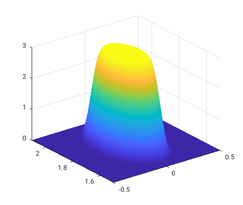
Here is a -continuous cutoff function which equals to when and when , and . Note that is compactly supported in the disk with center and radius . The height is taken as and the the thickness of the PML layer is fixed as . The fixed complex . For structures and the source term we refer to Figure 3.
(a)
(b)
Figure 3: (a) Structure; (b) source term.
We produce the “exact solution” (denoted by ) by the numerical approximation of the exact formulation 4-(6) with the discretization method of (7) (with 80 nodal points) introduced in [14]. The parameter here is chosen as , which is different from the PML method which is . The maximum meshsize is and the DtN map is approximated by a finite series
Then we compare the numerical result obtained by the PML method with different parameter ’s with the “exact solution”, on a straight line , which lies below the PML layer. Note that since the thickness is fixed, the parameter only depends on . Thus we replace the subscription by in this section. The relative error is defined as
Note that the meshes are exactly the same as for the “exact solutions” and the discretization method of () is introduced in [15] with also points.
We carry out the numerical methods for four different wavenumbers. Two wavenumbers satisfy Assumption 2, which are and ; and two do not satisfy this assumption, which are and . Numerical results with different ’s are listed in Table 1. We also plot the logarithm relative error against the parameter in Figure (a). From both Table 1 and Figure (a), the error decays exponentially at first, and the decay no longer days when it reaches . We give two possible reasons for this phenomenon. The first is the error from the finite element method with fixed meshes in both the “exact solutions” and the PML solutions. Note that since the convergence rate for the discretization methods introduced in [14, 15] is always very fast, we ignore the relative errors from these processes. The second reason is the increasing of errors due larger parameter ’s.
Table 1: Relative -errors different ’s and ’s.
E
E
E
E
E
E
E
E
E
e
E
E
E
e
E
E
E
e
E
E
E
e
E
E
E
e
E
E
E
e
E
E
E
e
E
E
E
e
E
E
(a)
(b)
Figure 4: (a) dependence of errors on the parameter ; (b) slopes with difference ’s.
It is interesting to see that even for wavenumbers which do not satisfy Assumption 2, the PML method also converges exponentially with respect to the parameter . This may imply that the error estimate is expected to be extended to these cases. We also observe an increasing of the slopes with larger ’s. We carry out line fittings for each curve in the exponentially decaying parts and the results are shown in Table 2 and Figure 4 (b). In Theorem 11 it is expected that the dependence of the slope is , the result shown in Figure 4 is even faster. This may come from the difference choices of another parameter , which is not very clear according to the discussions in this paper.
Table 2: Slopes with different ’s.
wavenumber
slopes
6 Further comments
The method introduced in this paper can be extended without major difficulty to the case with local perturbations in the periodic surface. However, we do not discuss this case in this paper since we would like to have simplified representations. For details we refer to [14]. This method can also be extended to locally perturbed periodic layers, but this may involve the guided modes which propagate along the periodic structures. We refer to [8] for some details for this case.
From numerical examples, for wavenumbers that do not satisfy Assumption 2 the convergence is also exponential. The decay rates for all the wavenumbers are much faster than expected (since from Theorem 11 the convergence depends on which is expected to be very small), which implies that the estimation in this paper maybe not optimal. Due to above reasons, the author has a conjecture that the convergence rate does not depend on thus it is easily extended to the case with Assumption 2. Since we are not able to prove that at present, it remains to be an open question.
Acknowledgment
This work is funded by the Deutsche Forschungsgemeinschaft (DFG, German Research Foundation) – Project-ID 258734477 – SFB 1173 and Project-ID 433126998. The idea to apply the perfectly matched layers to the periodic open waveguide problems was proposed by Prof. Sonia Fliss during a discussion. The author is grateful for her valuable suggestions that motivated this paper. The author is also grateful for Prof. Andreas Kirsch for his valuable suggestions in improving this paper.
References
[1]
T. Arens and R. Zhang.
A nonuniform mesh method for scattering problems in periodic
structures.
Preprint, 2021.
[2]
J.-P. Berenger.
A perfectly matched layer for the absorption of electromagnetic
waves.
Journal of Computational Physics, 114(2):185–200, 1994.
[3]
G. Bruckner and J. Elschner.
A two-step algorithm for the reconstruction of perfectly reflecting
periodic profiles.
19(2):315–329, 2003.
[4]
S. N. Chandler-Wilde and J. Elschner.
Variational approach in weighted Sobolev spaces to scattering by
unbounded rough surfaces.
SIAM. J. Math. Anal., 42:2554–2580, 2010.
[5]
S. N. Chandler-Wilde and P. Monk.
Existence, uniqueness, and variational methods for scattering by
unbounded rough surfaces.
SIAM. J. Math. Anal., 37:598–618, 2005.
[6]
S. N. Chandler-Wilde and P. Monk.
The pml for rough surface scattering.
Applied Numerical Mathematics, 59:2131–2154, 2009.
[7]
Z. Chen and H. Wu.
An adaptive finite element method with perfectly matched absorbing
layers for the wave scattering by periodic structures.
SIAM Journal on Numerical Analysis, 41(3):799–826, 2003.
[8]
S. Fliss, A. Kirsch, and R. Zhang.
The PML-method for a scattering problem for an open locally
perturbed periodic waveguide.
In preparation, 2021.
[9]
A. Kirsch.
Diffraction by periodic structures.
In L. Pävarinta and E. Somersalo, editors, Proc. Lapland
Conf. on Inverse Problems, pages 87–102. Springer, 1993.
[10]
A. Kirsch and R. Zhang.
Computation of the exceptional values for an open waveguide.
Preprint, 2021.
[11]
A. Lechleiter.
The Floquet-Bloch transform and scattering from locally perturbed
periodic surfaces.
J. Math. Anal. Appl., 446(1):605–627, 2017.
[12]
A. Lechleiter and D.-L. Nguyen.
Scattering of Herglotz waves from periodic structures and mapping
properties of the Bloch transform.
Proc. Roy. Soc. Edinburgh Sect. A, 231:1283–1311, 2015.
[13]
P. Li, H. Wu, and W. Zheng.
Electromagnetic scattering by unbounded rough surfaces.
SIAM J. Math. Anal., 43(3):1205–1231, 2011.
[14]
R. Zhang.
A high order numerical method for scattering from locally perturbed
periodic surfaces.
SIAM J. Sci. Comput., 40(4):A2286–A2314, 2018.
[15]
R. Zhang.
Numerical method for scattering problems in periodic waveguides.
https://arxiv.org/pdf/1906.12283.pdf, 2019.