Gauge Theory and the Analytic Form
Of The Geometric Langlands Program
Davide Gaiotto
Perimeter Institute
Waterloo, Ontario, Canada N2L 2Y5
Edward Witten
Institute for Advanced Study
Einstein Drive, Princeton, NJ 08540 USA
We present a gauge-theoretic interpretation of the “analytic” version of the geometric Langlands program, in which Hitchin Hamiltonians and Hecke operators are viewed as concrete operators acting on a Hilbert space of quantum states. The gauge theory ingredients required to understand this construction – such as electric-magnetic duality between Wilson and ’t Hooft line operators in four-dimensional gauge theory – are the same ones that enter in understanding via gauge theory the more familiar formulation of geometric Langlands, but now these ingredients are organized and applied in a novel fashion.
1 Introduction
Geometric Langlands duality as originally formulated by Beilinson and Drinfeld [1] is a relationship between categories associated to moduli spaces of fields on a Riemann surface . Many ingredients that enter in formulating and analyzing this duality are familiar in quantum field theory. In particular, two-dimensional conformal field theory plays a prominent role, as reviewed in [2]. The relation of geometric Langlands duality to quantum field theory can be understood more fully by formulating the subject in terms of a twisted version of super Yang-Mills theory [3]. From that point of view, geometric Langlands duality is deduced from electric-magnetic duality between the theory for a compact gauge group and the same theory based on the Langlands or GNO dual group (the complexifications of these groups will be called and ). Twisting of super Yang-Mills theory produces a four-dimensional topological field theory, which naturally [5, 6, 7] assigns a number (the partition function) to a four-manifold, a vector space (the space of physical states) to a three-manifold, and a category of branes or boundary conditions to a two-manifold.11 1 This idealized description does not take into account the fact that the complex Lie groups and and the associated moduli spaces are not compact. Because of this noncompactness, one likely gets only a partial topological field theory. Branes and spaces of physical states can be defined, but it is not clear that the integrals that formally would define partition functions associated to four-manifolds can really be defined satisfactorily. (A somewhat similar situation arises in Donaldson theory of four-manifolds, though the details are quite different: one does not get a complete topological field theory, as the partition function cannot be suitably defined for all four-manifolds.) The noncompactness also means that to define branes and spaces of physical states, one has to specify the allowed asymptotic behavior of a brane or a wavefunction. Each (reasonable) choice leads to a different version of the duality. Possibilities include the Betti and de Rham versions [4]. The usual geometric Langlands duality is a duality between the categories associated to two-manifolds.
Recently an analytic version of geometric Langlands duality has been discovered by Etingof, Frenkel, and Kazhdan [8, 9, 10], stimulated in part by a number of mathematical [11] and physical [12] developments. Rather than categories and functors acting on categories, one considers a Hilbert space of quantum states and self-adjoint operators such as quantum Hitchin Hamiltonians acting on this Hilbert space. Very roughly, the usual formulation of geometric Langlands duality involves deformation quantization of the algebra of holomorphic functions on the moduli space of Higgs bundles on a Riemann surface , while the analytic version of the theory involves ordinary quantization of the same moduli space, viewed now as a real symplectic manifold. As usual, quantization means that a suitable class of smooth functions – in general neither holomorphic nor antiholomorphic – become operators on a Hilbert space. See also [14, 19, 15, 13, 16, 18, 20, 17] for prior work on the gauge theory interpretation of the spectrum of quantum Hitchin Hamiltonians.
The goal of the present article is to place the analytic version of geometric Langlands duality in the gauge theory framework. The first step is simply to understand what one should do in that framework to study the quantization of viewed as a real symplectic manifold, as opposed to its deformation quantization when viewed as a complex symplectic manifold. The basic idea here is that the problem of quantization of a real symplectic manifold is part of the -model of a suitable complexification of (if such a exists) [21]. We have explored this construction in more detail elsewhere as background to the present article [22]. For the application to geometric Langlands, we want to quantize the Higgs bundle moduli space viewed as a real symplectic manifold with one of its real symplectic structures. A suitable complexification of is simply the product of two copies of with opposite complex structures. With this as the starting point for understanding the quantization of , we will show that the analytic version of geometric Langlands can be understood by assembling in a novel fashion the same gauge theory ingredients that have been used previously for understanding the more traditional version of geometric Langlands.
The organization of this article is as follows. In Section 2, we explain the basic setup for formulating the analytic version of geometric Langlands duality in terms of super Yang-Mills theory. In Section 3, we explain the predictions of electric-magnetic duality for the joint eigenvalues of the Hitchin Hamiltonians, and in Section 4, we analyze Hecke or ’t Hooft operators and the dual Wilson operators. In Section 5, we show that the joint eigenfunctions of the Hitchin Hamiltonians satisfy a quantum-deformed WKB condition. In Section 6, we discuss the quantization of real forms of the Higgs bundle moduli space. Starting in Section 7, we use chiral algebras that arise at junctions between supersymmetric boundary conditions in order to build an interesting class of wavefunctions, whose spectral decomposition is controlled by the geometry of -dual boundary conditions. These wavefunctions are typically not eigenfunctions, but we expect them to play a useful role in the context of the analytic version of the geometric Langlands program. In Section 8, we study Hecke operators by relating them to spectral flow automorphisms of Kac-Moody algebras. The relationship between Hecke operators and spectral flow automorphisms of chiral algebras, which is important in this analysis, has been observed previously from a different but related perspective [14]. In Section 9, we explore in detail an example with remarkable properties, leading to a wavefunction which intertwines three copies of the Hitchin Hamiltonians and Hecke operators for .
Some further issues are treated in appendices. In Appendix A, we analyze the cohomology of local operators inserted along the canonical coisotropic brane. The result shows that Hitchin’s classical integrable system can be quantized. In Appendix B, we explain that electric-magnetic duality together with positivity of the Hilbert space inner product in quantization of imply that the intersections of the varieties and that parametrize holomorphic and antiholomorphic opers must be isolated and transverse (as conjectured in [8] and proved in some cases). We further point out that electric-magnetic duality implies a natural normalization for the joint eigenfunctions of the Hitchin Hamiltonians and argue that the Hilbert space norm of a normalized wavefunction is given by, roughly speaking, the torsion of the associated oper bundle. In Appendix C, we explore some examples of differential equations satisfied by line operators. In Appendix D, we construct a local model to analyze the singular behavior of the eigenfunctions of the Hitchin Hamiltonians along the divisor of not very stable bundles.
Throughout this article, is a Riemann surface of genus . All considerations can be naturally extended to the case of bundles with parabolic structure, but for simplicity we will omit this generalization (which has been developed in [8, 9, 10]). With sufficiently many parabolic points, there is a quite similar theory for genus . The cases without parabolic structure (or with too few parabolic points for ) require a different treatment because any low energy description requires gauge fields, not just -model fields.
2 Basic Setup
This section is devoted to an explanation of the basic framework in which we will study the analytic version of geometric Langlands, and a review of part of the background.
2.1 Quantization Via Branes
Here we briefly summarize some things that have been described more fully elsewhere [21, 22]. First we explain deformation quantization via branes and then we describe quantization.
Let be a complex symplectic manifold, with complex structure and holomorphic symplectic form . We view as a real symplectic manifold with the real symplectic form . We assume that is such that a quantum -model with target exists (as an ultraviolet-complete quantum field theory), and we consider the -model obtained by twisting this -model in a standard way. It is not known in general for what class of ’s the -model does exist, but a sufficient condition is believed to be that the complex symplectic structure of can be extended to a complete hyper-Kahler structure. The examples important for the present article are the cases that is the Higgs bundle moduli space , which indeed admits a complete hyper-Kahler metric [23], or a product (with opposite complex structures on the two factors and complex conjugate symplectic structures), which of course also has a complete hyper-Kahler metric.
In general, the -model of a symplectic manifold , in addition to the usual Lagrangian branes whose support is middle-dimensional in , can have coisotropic branes, supported on a coisotropic submanifold of that is above the middle dimension [24]. The simplest case and the only case that we will need in the present article is a rank 1 coisotropic -brane whose support is all of . Let be the -field of the -model, and consider a brane with support whose Chan-Paton or bundle is a line bundle , with a unitary connection of curvature . The Kapustin-Orlov condition for this data to define an -brane is that should be an integrable complex structure on . Two solutions of this condition immediately present themselves. One choice is , . The brane constructed this way is what we will call the canonical coisotropic -brane, . A second choice is , . This leads to what we will call the conjugate canonical coisotropic -brane, . To treat the two cases symmetrically, in the present article it is convenient to take22 2 This choice was made in [21]. However, when only one of , is relevant, it can be simpler to take , . , . This choice is only possible if there exists a complex line bundle with curvature . In our application to the Higgs bundle moduli space, is cohomologically trivial, so exists and can be assumed to be topologically trivial.
Now consider the algebra (which in physical terms is the space of open strings, with an associative multiplication that comes by joining of open strings). Suppose that , where we keep fixed and vary . For , reduces to the commutative algebra of holomorphic functions on in complex structure . In order , the multiplication law in differs from the commutative multiplication law in by the Poisson bracket . So can be viewed as a deformation quantization of . is related in the same way to the commutative algebra of holomorphic functions on in complex structure , or equivalently antiholomorphic functions in complex structure , and can be viewed as a deformation quantization of .
Generically, deformation quantization is a formal procedure that has to be defined over a ring of formal power series in . When a quantum -model of exists, it is expected that can be set to a complex value (such as 1), rather than being treated as a formal power series variable. In the present example, one can give a more direct explanation of this. The Higgs bundle moduli space has a symmetry, rescaling the Higgs field by , . This operation rescales in the same way. Of course, this is possible only because is cohomologically trivial. The ring is generated by functions that scale with a definite degree (namely the Hitchin Hamiltonians) and the scaling symmetry implies that all the relations in the deformed ring are polynomials in the deformation parameter . Hence it makes sense to set . Similar remarks will apply when we consider quantization rather than deformation quantization, given that the important branes considered are -invariant: the scaling symmetry will imply that certain semiclassical formulas are actually exact.
Deformation quantization is particularly interesting if is an affine variety, with lots of holomorphic functions. As already noted, in our main examples, will be or . is far from being an affine variety. The ring in the case is simply the ring of functions on the base of the Hitchin fibration; in other words, the global holomorphic functions on are simply the functions of Hitchin’s Poisson-commuting Hamiltonians. Hitchin’s Poisson-commuting Hamiltonians can be quantized to commuting differential operators, acting on sections of the line bundle , where is the canonical bundle of . This was shown by Hitchin [25] for and by Beilinson and Drinfeld [1] in general. In particular, the ring is commutative. The fact that the Poisson-commuting classical Hamiltonians can be quantized to commuting differential operators can also be seen in the gauge theory language, as we will discuss in Section 2.4 and Appendix A. For , deformation quantization just gives the product of this answer with its complex conjugate.
In the present article, we are really interested in quantization rather than deformation quantization. How to modify the story just described to encompass quantization has been explained in [21, 22]. Suppose that is a real symplectic manifold, with symplectic form , that we wish to quantize. (In our main application, will be , viewed as a real symplectic manifold, and will be .) If has a complexification that obeys certain conditions, then quantization of is part of the -model of . should be a complex symplectic manifold with a holomorphic symplectic form whose restriction to is . Moreover, should have an antiholomorphic involution33 3 An involution is an automorphism whose square is 1. with as a component of its fixed point set. These conditions imply that . For the example , the antiholomorphic involution is the map that exchanges the two factors. Finally, the quantum -model of must exist. Under these conditions, a choice of a prequantum line bundle , in the sense of geometric quantization,44 4 A prequantum line bundle over a symplectic manifold with symplectic form is a complex line bundle with a unitary connection of curvature . determines an -brane with support . (The details of this depend on the choice that was made in satisfying the condition to define the brane . We will be specific in Section 2.2.) The -model answer for the Hilbert space obtained by quantizing with symplectic structure and prequantum line bundle is . The definition of the hermitian inner product on is described in Section 2.2.
is always a module for . This can be described by saying that those functions on that can be analytically continued to holomorphic functions on are quantized to give operators on . In addition, under mild conditions, a correspondence55 5 A correspondence between and itself is simply a Lagrangian submanifold of , where and are two copies of , with respective symplectic structures and . A holomorphic correspondence between and itself is defined similarly. between and itself that can be analytically continued to a holomorphic correspondence between and itself can be quantized in a natural way to give an operator on . In our main example with , the ring will be relatively small, consisting of polynomials in the holomorphic and antiholomorphic Hitchin Hamiltonians. By way of compensation, there is an ample supply of correspondences – the Hecke correspondences – that will provide additional operators on . Quantizing these correspondences is simple because of the scaling symmetry that was invoked in the discussion of deformation quantization.
We have described this in the context of two-dimensional -models, as is appropriate for quantization of a fairly general real symplectic manifold . However, in the particular case that is the Higgs bundle moduli space for gauge group on a Riemann surface , a four-dimensional picture is available and gives much more complete understanding. For this, the starting point is super Yang-Mills theory, in four dimensions, with gauge group . One restricts to four-manifolds of the form , where is an arbitrary two-manifold but is kept fixed. At low energies, the four-dimensional gauge theory reduces for many purposes, assuming that has trivial center, to a supersymmetric -model on with target [26, 27]. A certain twisting of the theory in four dimensions produces a topological field theory66 6 This is really a partial topological field theory, as remarked in footnote 1. that, when we specialize to four-manifolds of the form , reduces to an -model on with target . The brane of the -model originates in the four-dimensional gauge theory as a boundary condition that is a simple deformation of Neumann boundary conditions for the gauge field, extended to the whole supermultiplet in a half-BPS fashion; see Section 12.4 of [3].
The four-dimensional lift of the boundary condition has an interesting and important feature. Though it is a brane in an -model that has full four-dimensional topological symmetry, the definition of the brane depends on a choice of complex structure of . The deformed Neumann boundary condition is a holomorphic-topological local boundary condition for the four-dimensional topological field theory.77 7 Concretely, the boundary condition breaks some of the bulk supersymmetries of the physical theory. As a consequence, some translation generators which are -exact in the bulk cease to be -exact in the presence of the boundary and the boundary condition is not topological in the four-dimensional sense. Another explanation of the dependence of on a choice of complex structure is simply that is defined with , whose definition depends on the complex structure of . See the beginning of Section 2.2 for a statement of which structures on do or do not depend on a choice of complex structure. Boundary local operators supported at a point can depend holomorphically on , even though they depend topologically on the one remaining boundary direction. This will be important whenever we discuss the four-dimensional lift of our constructions. Although the -model has full four-dimensional topological invariance, in the presence of the brane , only two-dimensional topological invariance is available. For example, in proving the commutativity of the Hitchin Hamiltonians and the Hecke operators, we will use only two-dimensional topological invariance.
If has a nontrivial center , then the assertion about a reduction to a -model must be slightly modified. A more precise statement is that upon compactification on , the four-dimensional gauge theory reduces, for many purposes, to the product of a -model with target and a gauge theory with the finite gauge group (acting trivially on ). This finite gauge group will play no role until we want to compute the eigenvalues of Hitchin Hamiltonians and Hecke operators, so in much of the following it will not be mentioned.
A purely two-dimensional description via a -model with target (possibly extended by the finite gauge group) is useful for many purposes. But information is lost in the reduction to two dimensions, and the four-dimensional picture is needed for a complete account of the duality.88 8 To be more precise, a complete formulation of the duality is possible in four dimensions. A fuller explanation of the duality comes from a certain starting point in six dimensions [28]. In standard mathematical treatments, an analogous statement is that geometric Langlands duality must be formulated in terms of the “stack” of -bundles or of local systems, rather than in terms of a finite-dimensional moduli space. There is a simple relation between the two statements. It was shown by Atiyah and Bott [29] that the space of all -valued connections on a smooth -bundle , with the action of the group of complexified gauge transformations, provides a model of the stack of holomorphic -bundles. That is because the part of any connection gives (or more precisely its complexification) a complex structure, making it a holomorphic bundle over . A gauge field on a -bundle over determines, in particular, a family, parametrized by , of gauge fields on . So any such connection determines a map from to the stack of bundles over . Thus super Yang-Mills theory on can be understood as a supersymmetric -model on with the target being the stack of bundles over . (In this formulation, the theory is a two-dimensional supersymmetric gauge theory on coupled to matter fields. The matter fields are gauge fields on and their superpartners, and the gauge group is the group of maps of to the finite-dimensional group . A gauge transformation in the two-dimensional theory is a map from to ; in the four-dimensional description, this is interpreted as a map of the four-manifold to . To keep these statements simple, we have assumed that all bundles are trivialized.) The mathematical statement that the correct formulation involves stacks corresponds to the quantum field theory statement that the correct formulation is in four dimensions.
2.2 Quantizing A Complex Manifold
We view as a complex manifold in the complex structure, called by Hitchin [23], in which it parametrizes Higgs bundles over . is one of a triple of complex structures that, along with the corresponding Kahler forms , make a hyper-Kahler structure on . In complex structure , parametrizes flat bundles over with structure group . Complex structure and the corresponding holomorphic symplectic form are topological in the sense that they depend on only as an oriented two-manifold, while the other structures , , and depend on a choice of complex structure on .
The complex symplectic form of , in complex structure , is . We want to view as a real symplectic manifold with the real symplectic structure , and quantize it.
As we have explained in Section 2.1, the first step in quantizing any real symplectic manifold via branes is to pick a suitable complexification of it. Here we are in a special situation, since is actually a complex manifold. In such a case, there is a standard way to proceed, described in Section 5 of [22].
In spelling out the details, rather than specializing to , we will consider the general problem of quantizing a complex symplectic manifold viewed as a real symplectic manifold. In this particular context, we will write (rather than ) for the manifold that is being quantized. The reason for this is that is our generic notation for a complex symplectic manifold, and in the approach to quantization that we will describe, the complex symplectic structure plays an important role. Our notation is particularly natural in the “unfolded” version of the construction (see fig. 1 below). Hopefully, this usage will cause no confusion.
For a complexification of , we take , where and are two copies of , with opposite complex structures and . The complex structure of is thus a direct sum . The involution that exchanges the two factors is antiholomorphic, and its fixed point set is a copy of , embedded as the diagonal in . We endow with the complex symplectic form ; in other words, the symplectic form of is on the first factor and on the second factor. This definition ensures that the restriction of to the diagonal is . Suppose that the complex symplectic structure of can be extended to a complete hyper-Kahler metric. Then the complex symplectic structure of can likewise be extended to a complete hyper-Kahler metric, namely a product hyper-Kahler metric on . So all conditions are satisfied, and the -model of with real symplectic form is suitable for quantizing with the symplectic structure .
To define coisotropic branes, we have to satisfy the Kapustin-Orlov condition that should be an integrable complex structure. In doing so, we will take , as this will make it possible to treat the two factors of symmetrically. Since the complex structures of and are respectively and and the -model symplectic structures are respectively and , we can define canonical coisotropic branes and on and by taking in each case a bundle with curvature . (In our application to the Higgs bundle moduli space, is exact and , so a topologically trivial line bundle over with curvature exists and is unique up to isomorphism.) One then defines on the product brane , with bundle . We also define a Lagrangian brane supported on with trivial bundle. Following the general logic, the Hilbert space for quantization of with the real symplectic structure is . The prequantum line bundle in this situation is . Since has curvature , has curvature , so it is an appropriate prequantum line bundle for quantization of with symplectic structure .
However, this definition has a useful variant. To compute , we study the model with target on a strip , with boundary conditions set by of the left boundary of the strip and by on the right boundary, as in fig. 1(a). The two factors of are decoupled in the bulk of the -model, since the metric on is a product; they are also decoupled on the left boundary, since the brane is likewise a product. So away from the right boundary of the strip, we can think of as having two sheets, one of which is mapped to and one to , as in the figure. The two sheets are coupled only on the right boundary, where, as is supported on the diagonal in , the two sheets are “glued together” and map to the same point in . This suggests that we should “unfold” the picture (fig. 1(b)). After this unfolding, we simply have a single sheet of twice the width that is mapped to a single copy of . Unfolding reverses the orientation of one of the two sheets of the folded picture, and this orientation reversal changes the sign of the -model symplectic form. In the folded picture, the -model symplectic form was on and on ; hence after unfolding, the -model symplectic form is everywhere. In other words, the unfolded picture involves the ordinary -model of a single copy of with symplectic form . Before unfolding, the branes and both have bundles with curvature . Reversing the orientation of replaces the bundle of a brane with its dual (or its inverse, in the rank 1 case), and so reverses the sign of the curvature. Hence in the unfolded picture, the boundaries are labeled by branes and whose respective bundles are lines bundles and with curvatures and . These are the conjugate canonical coisotropic branes that were introduced in Section 2.1. The prequantum line bundle is still . is a deformation quantization of the commutative algebra of holomorphic functions on , and is similarly a deformation quantization of the algebra of antiholomorphic functions on . What in the folded picture was becomes in the unfolded picture .
With either description of , we need to define a hermitian product on . For definiteness we use the folded language.99 9 For more detail on the following, see Section 2.7 of [22]. Topological field theory would give us in general a nondegenerate bilinear (not hermitian) pairing between and its dual space . To get a hermitian pairing on , we need to compose this bilinear pairing with an antilinear map from to . Such a map in the underlying physical theory is provided by the symmetry . But is not an -model symmetry; it maps the -model to a conjugate -model with the opposite sign of the symplectic form. The involution that exchanges the two factors of also exchanges the -model with its conjugate, since it is antisymplectic (it reverses the sign of the -model symplectic form), so is an antilinear symmetry of the -model. Finally, because the branes and are -invariant, maps to and we can define a nondegenerate hermitian pairing on by
| (2.1) |
For general -invariant branes, such a pairing is not positive-definite. For the specific case of quantizing a cotangent bundle, which is our main example on the -model side, one expects positivity. The -model analog of this construction uses an antiholomorphic (not antisymplectic) involution . Positivity of the pairing in this case is subtle and is discussed in Appendix B.
In the folded picture, and therefore also exchanges the two factors of ; in the unfolded picture, they exchange the two ends of the strip. Exchanging the two ends of the strip reverses the orientation of the strip and therefore would change the sign of . Hence in a description with , the definition of the inner product is less natural (one would need to accompany with a -field gauge transformation). That is why we took in solving the Kapustin-Orlov conditions for rank 1 coisotropic branes.
2.3 Quantizing The Higgs Bundle Moduli Space
For our application to quantization of for some gauge group and Riemann surface , we really want to study the four-dimensional version of this construction. This means that we study the super Yang-Mills theory, with gauge group , on , where is the strip of fig 1(b). The boundary conditions on the left and right of the strip are set by the gauge theory versions of and . A detailed description of in four-dimensional gauge theory language was given in Section 12.4 of [3]. We can describe a Higgs bundle on by a pair , where is gauge field, that is, a connection on a -bundle , and is a 1-form valued in the adjoint bundle . In this description, is obtained from by (suitably extended to the rest of the four-dimensional supermultiplet). This is a familiar involution of the Higgs bundle moduli space that acts holomorphically in complex structure and antiholomorphically in complex structures and .
Although we have used machinery of gauge theory and branes to construct a Hilbert space associated to quantization of , the actual output of this construction is completely unsurprising. A dense open set in is a cotangent bundle , where is the moduli space of semistable holomorphic -bundles over . Geometric quantization – or simply elementary quantum mechanics – suggests that the Hilbert space that we should associate to quantization of should be the space of half-densities on .
The reason to speak of half-densities rather than functions is that on a general smooth manifold without some choice of a measure,1010 10 The space actually does have a natural measure, namely the one associated to its real symplectic structure when viewed as a moduli space of flat bundles over with compact structure group . This is also the measure induced by its embedding in the hyper-Kahler manifold . However, this measure is not part of the -model and does not naturally appear in -model constructions such as the definition of the Hilbert space . there is no way to integrate a function so there is no natural Hilbert space of functions. A density on a manifold is a section of a trivial real line bundle and can be written locally in any coordinate system as , where is a function and is a measure, not a differential form. has a square root , also trivial, whose sections are locally described in a given coordinate system by functions that transform under a change of coordinates in such a way that is invariant. It is convenient to formally write
| (2.2) |
for a section of . Complex-valued half-densities, which are described by the same formula where locally is a complex-valued function, form a Hilbert space in an obvious way:
| (2.3) |
Now, motivated by the application to the complex manifold , let us describe the bundle of densities or half-densities on a complex manifold . If has complex dimension and local holomorphic coordinates , then is a density on , in other words a section of . On the other hand, is a section of the holomorphic canonical bundle , and is a section of the complex conjugate line bundle (which can also be viewed as the canonical line bundle of if is endowed with the opposite complex structure). So can be identified with ; more precisely , that is, is the complexification of , the bundle of complex-valued densities. Similarly always has a square root at least locally, and for any choice of local square root of , we have ; more precisely , that is, is the bundle of complex-valued half-densities. As long as is the complex conjugate of , this relation holds for any choice of .
In Section 3 of [22], criteria were described under which brane quantization of , with its standard symplectic structure as a cotangent bundle, leads to a Hilbert space of half-densities on . Beyond requiring that has a complexification that is suitable for brane quantization, the necessary condition is that should be the cotangent bundle of a complexification of (and should have the natural complex symplectic structure of a cotangent bundle). This condition is automatically satisfied if and are already complex manifolds and is defined as the product of two copies of with opposite complex structures.
The Higgs bundle moduli space contains as a dense open set, but is not actually isomorphic to . One would not expect a measure zero discrepancy to be important in the definition of a Hilbert space of wavefunctions. The construction in [22] maps the Hilbert space obtained in quantizing to a space of half-densities on without requiring that is literally all of .
The Hilbert space of half-densities on was already introduced in [8] without any reference to branes and -models or gauge theories. The interpretation via branes makes it possible to apply electric-magnetic duality and other methods of gauge theory. We will see an example next in discussing the Hitchin Hamiltonians.
2.4 Hitchin Hamiltonians
As we have seen, in brane quantization of a complex manifold (such as ) that we quantize as a real symplectic manifold, the Hilbert space has an unfolded description as . admits a left action of1111 11 In the folded picture, we have instead a left action of both algebras and . A left action of an algebra is the same as a right action of the opposite algebra. (The notion of the opposite algebra is explained in Appendix C of [22].) Unfolding reverses the orientation of one sheet in fig. 1 and hence replaces one of the two algebras with its opposite. Of course, which algebra acts on the left and which on the right depends on some choices. None of this will be important in the present article as and will be commutative and hence isomorphic to their opposites. and a right action of . and are quantum deformations of the commutative rings and of holomorphic functions on . In a general case, these deformations can be noncommutative, but in the particular case of , it turns out that and are commutative and hence there is no distinction between a left action and a right action.
Concretely, the ring of holomorphic functions on in complex structure is simply the ring of functions on the base of the Hitchin fibration [23, 30]. Consider a solution of Hitchin’s equations, where is a connection on a -bundle and is a -form valued in . Let be the holomorphic Higgs field, that is, the part of . Hitchin’s equations give . So if be an invariant polynomial on the Lie algebra of , homogeneous of some degree , then is a holomorphic section of (with the canonical bundle of ; we will also set ). Given any -form on with values in , we can define
| (2.4) |
This is a holomorphic function on and depends only on the cohomology class of in . The dimension of is , and this is the number of linearly independent functions for a given . For , the ring of holomorphic functions on is generated by the where . More generally, a simple Lie group of rank has independent Casimir operators, corresponding to homogeneous polynomials , of various degrees, and is generated by the . For example, if , we can take the generating polynomials to be , .
The functions are Poisson-commuting, since the holomorphic symplectic structure of in complex structure is such that and are conjugate variables, and in particular any functions constructed from only (and not ) are Poisson-commuting. These Poisson-commuting functions are the Hamiltonians of Hitchin’s classical integrable system.
The quantum deformation from to is unobstructed in the sense that every element of can be quantum-deformed to an element of . This statement means, concretely, that if is an invariant polynomial on homogeneous of some degree , and is a corresponding Hitchin Hamiltonian, then there is a differential operator , acting on sections of , whose leading symbol is equal to . The passage from to is not entirely canonical, since specifying the desired leading symbol of leaves one free to add to a globally-defined holomorphic differential operator of degree less than . For , one can take to be of degree 2, and then the only globally-defined holomorphic differential operators of lower degree are the operators of degree 0 – the complex constants. For groups of higher rank, in general there are more possibilities. Mathematically, the fact that the deformation is unobstructed follows from the fact that, for any simple , , by virtue of which there is no potential obstruction in the deformation. A gauge theory version of this argument is given in Appendix A, elaborating on a previous discussion in [3].
From the point of view of the -model, or the underlying gauge theory, the deformation from to arises from an expansion in powers of . This expansion terminates after finitely many steps, since we define to consist of functions whose restriction to a fiber of the cotangent bundle is a polynomial. A specific definition of the -model or the gauge theory gives a specific recipe for passing from to , but this depends on data (such as a Riemannian metric on , not just a complex structure) that is not part of the -model.
Next we would like to explain why is commutative, like . This was originally proved for by Hitchin [25] and for general simple by Beilinson and Drinfeld [1]. We will give a four-dimensional explanation similar to that in [3]. Of course the same considerations apply to . As a warmup, we first explain why commutes with . This is clear from the fact (fig. 2(a)) that an element is inserted on the left boundary of the strip, while an element is inserted on the right boundary. In two-dimensional topological field theory, we are free to slide these insertions up and down along the boundary independently. There is no meaningful relative time-ordering between the two boundary insertions and they must commute. By contrast, consider the insertion of a pair of elements (fig 2(b)). Here, as a general statement in two-dimensional topological field theory, there is a meaningful time-ordering between and . If we try to slide one of them past the other in time, there may be a discontinuity when they cross, and therefore in general we may have . However, in the present problem, we are really not in two dimensions but in four dimensions; there are two extra dimensions, making up the Riemann surface , that are not shown in the figure. The definition of in eqn. (2.4) depended only on the cohomology class of in . We can choose a representative with support in an arbitrarily selected small open ball in . Therefore, when we consider a pair of elements , we can assume that they are represented by operators that have disjoint support in . Hence we can slide the two operators up and down past each other in the two-dimensional picture of fig. 2(b) without any singularity. Accordingly, they commute.
We can elaborate slightly on the four-dimensional origin of the quantum Hitchin hamiltonians. The integrands in the classical Hitchin Hamiltonians depend holomorphically on . As we review in Section 8, the quantum Hitchin Hamiltonians can also be written as
| (2.5) |
in terms of certain differential operators which act on the bundle locally at a point and depend holomorphically on . We identify as the action of a four-dimensional boundary local operator . The holomorphic-topological nature of the boundary condition insures that such boundary local operators commute in the topological direction and have non-singular operator product expansion (OPE) with each other.
As was explained in Section 2.3, the quantum Hilbert space is the space of half-densities on , or equivalently the space of sections of . We recall that this happens because brane quantization of is equivalent to quantizing it as a cotangent bundle . In quantizing a cotangent bundle , a function whose restriction to a fiber of the cotangent bundle is a polynomial of degree becomes a differential operator of degree acting on half-densities on . If, as in the case of interest here, is a complex manifold, then more specifically holomorphic functions on become holomorphic differential operators on . From a holomorphic point of view, one usually says that holomorphic functions on (with polynomial dependence on the fibers) become holomorphic differential operators acting on sections of . (The role of is explained from a -model point of view in [22], Section 3.2 and Appendix C.) In the case of the Hitchin Hamiltonians, the fact that they can be quantum deformed to differential operators acting on sections of , and not on sections of any other holomorphic line bundle, is part of the standard story [25, 1]. However, the antiholomorphic line bundle is invisible to a holomorphic differential operator, since its transition functions are antiholomorphic and commute with holomorphic differential operators. So the holomorphic differential operators that are obtained by deformation quantization of holomorphic functions on can naturally act on , or equivalently on the bundle of half-densities. Similarly, under deformation quantization, antiholomorphic functions on become antiholomorphic differential operators that can act on .
So and become, respectively, algebras of holomorphic and antiholomorphic differential operators acting on half-densities on . From this point of view, the statement that and commute just reflects the fact that holomorphic differential operators commute with antiholomorphic ones.
2.5 The Duals Of The Coisotropic Branes
In order to be able to apply duality to this problem, we need one more ingredient. We need to understand the duals of the -branes and in the -model of . To be specific, here we mean the -model in the complex structure that is called in [23], in which parametrizes flat bundles over with structure group . We denote the connection on the flat bundle as , where are the unitary connection and Higgs field that appear in Hitchin’s equations. A general -brane is a coherent sheaf, or a complex of coherent sheaves, on . However, the -branes and have additional properties that imply that the dual -branes must be rather special. To explain this, we recall that the Higgs bundle moduli spaces are hyper-Kahler manifolds, with complex structures that obey the usual quaternion relations, and a triple of corresponding Kahler forms and complex symplectic forms , etc. Geometric Langlands duality in general maps the -model of with symplectic structure to the -model of in complex structure . When we speak of the -model or the -model without further detail, these are the models we mean. A generic brane in either of these models is merely an -brane or -brane of the appropriate type. However, many of the branes that are most important in geometric Langlands have additional properties. For example, a brane supported on a point in is a brane of type , that is, it is a -brane in each of complex structures , and (or any linear combination). The dual of a brane of type is a brane of type ; in the case of the Higgs bundle moduli space, the dual of a rank 1 brane supported at a point is a brane supported on a fiber of the Hitchin fibration, with a rank 1 flat bundle. These branes are the Hecke eigensheaves which are central objects of study in the geometric Langlands program; they will be discussed in Section 5. In the case at hand, and are branes of type ; they are -branes of types and , by virtue of the Kapustin-Orlov conditions for coisotropic branes, and they are -branes of type , because the curvature of their bundles is of type in complex structure , so that those bundles are holomorphic in complex structure . In general, the dual of a brane of type is a brane of type , so the duals of and will be branes of that type. The simplest kind of brane of type is given by the structure sheaf of a complex Lagrangian submanifold in complex structure . In more physical language, these are branes supported on a complex Lagrangian submanifold with a trivial bundle. And indeed, the duals of and are of this type. These duals were first identified (in a different formulation) by Beilinson and Drinfeld [1], with the help of conformal field theory at critical level . A gauge-theory explanation involves duality between the D3-NS5 and D3-D5 systems of string theory [31].
The complex Lagrangian submanifold supporting the dual of parametrizes flat bundles which satisfy a “holomorphic oper” condition. We will denote it as . Similarly, the dual of is supported on a complex Lagrangian submanifold that parametrizes flat bundles which satisfy an “antiholomorphic oper” condition.
The holomorphic oper condition can be stated rather economically as a global constraint on the holomorphic type of the bundle, i.e. on the part of , as we will do here, or in a more local way, as we will do in Section 2.6. Both formulations are standard mathematically. In a four-dimensional gauge theory, -duality maps a deformed Neumann boundary condition to a deformed “Nahm pole” boundary condition, which imposes directly the local constraints [31].
One general way to define a complex Lagrangian submanifold of is to consider all flat bundles with some fixed holomorphic type. Specifying the holomorphic type of a bundle is equivalent to specifying the part of . Here and in several analogous cases considered momentarily, we place no constraint on the part of the connection except that the full connection should be flat. While preserving the flatness of the connection on , we are free to add to the part of the connection an arbitrary -closed form representing an element of . The dimension of this space is half the dimension of , so flat bundles of a specified holomorphic type are a middle-dimensional submanifold of . is a complex Lagrangian submanifold, because the holomorphic symplectic structure of in complex structure is a pairing between the and parts of and vanishes if the part is specified. Once one picks a base point in , is isomorphic to the vector space .
We can define a second family of complex Lagrangian submanifolds, in the same complex structure on , by specifying the antiholomorphic structure of a flat bundle. This amounts to specifying the part of , and letting the part vary. It leads to a complex Lagrangian submanifold for the same reasons as before. It may come as a slight surprise that fixing either the or the part of is a holomorphic condition in complex structure . Indeed, complex structure on the Higgs bundle moduli space is not sensitive to the complex structure of the two-manifold , and treats the and parts of in a completely symmetric way.
The submanifolds and can be defined by specifying a particular choice of the holomorphic or antiholomorphic structure of a flat bundle. First we explain the definition for the case . For this group, an oper is a flat bundle that, as a holomorphic bundle, is a nontrivial extension of by :
| (2.6) |
There is a unique such nontrivial extension, up to isomorphism. The family of flat bundles of this holomorphic type is therefore a complex Lagrangian submanifold that we will call . In making this definition, we have made a choice of , or equivalently a choice of spin structure on . Indeed, for , the definition of an oper depends on such a choice of spin structure (though we do not indicate this in the notation for ). We return to this point in Section 2.7.
It is possible to give a simple description of once one picks a base point, that is, a particular bundle of oper type with flat connection . In deforming as an oper, we may as well keep the part of fixed, since we are required to keep it fixed up to a complex gauge transformation. But we can modify the part of . To do this while preserving the flatness of , we add to a -closed -form, that is, an element of . Using the exact sequence (2.6), one can show that is isomorphic to the space of quadratic differentials on . This is the base of the Hitchin fibration for , so is isomorphic to the base of the Hitchin fibration. This isomorphism is not entirely canonical as it depends on the choice of a base point in . A similar reasoning applies for other groups.
Similarly, an antiholomorphic oper for , or anti-oper for short, is a flat bundle that, antiholomorphically, is a nontrivial extension of by :
| (2.7) |
The family of such flat bundles is another complex Lagrangian submanifold, which we will call . It is noncanonically isomorphic to the base of the Hitchin fibration, with the opposite complex structure.
In general, if is a simple complex Lie group, there is a notion of a “principal embedding” of Lie algebras . For example, if , the principal embedding is such that the -dimensional representation of transforms irreducibly under ; the corresponding principal subgroup is a copy of or depending on whether is even or odd. For brevity we will sometimes ignore this subtlety and refer simply to a principal subgroup, though the global form of the group is sometimes .
A oper is a flat bundle that, as a holomorphic bundle, is equivalent to a principal embedding of an oper bundle, that is, a principal embedding of a rank two bundle that is a nontrivial extension of the form in eqn. (2.6). For , this means that an oper bundle is, holomorphically, the symmetric tensor power of such a nontrivial extension, and therefore has a subbundle isomorphic to :
| (2.8) |
(and a filtration by powers of ). Again, the part of the connection on is not restricted except by requiring the full connection to be flat. Similarly an antiholomorphic oper is a flat bundle that, as an antiholomorphic bundle, is equivalent to a principal embedding of an antiholomorphic oper bundle.
At the -model level, the duals of and are the structure sheaves of and ; that is, they are rank 1 branes and supported on and with trivial bundles.
2.6 The Local Constraints
To describe a more local characterization of an oper, we consider first the case . The extension structure of implies the existence of a global holomorphic section of . Denote as the part of the connection. The -invariant combination is a global holomorphic function on . This function must be non-zero: if it vanished, we could write and would define a holomorphic flat connection on , which does not exist (for of genus greater than 1 or in lower genus in the presence of parabolic structure).
Without loss of generality, we can normalize so that . This fixes up to sign. The local version of the holomorphic oper condition for is precisely the condition that admits a globally defined holomorphic section such that .
Taking a derivative, we have and thus satisfies a second order differential equation
| (2.9) |
for some “classical stress tensor” on . Under a change of local coordinate on , transforms as a stress tensor, not as a quadratic differential. Not coincidentally, eqn. (2.9) can be viewed as a classical limit of the Belavin-Polyakov-Zamolodchikov (BPZ) differential equations for the correlator of a degenerate field in two-dimensional conformal field theory. The classical stress tensor can be used to define a set of generators of the algebra of holomorphic functions on the oper manifold, consisting of functions of the form
| (2.10) |
with being a -form with values in .
The case of can be analyzed similarly. In this case, the oper structure of (eqn. (2.8)) implies the existence of a global holomorphic section of . Then is a global holomorphic function on which cannot vanish, for a similar reason to what we explained for . We can normalize so that ; this uniquely fixes , up to the possibility of multiplying by an root of 1. Since , we learn that satisfies a degree differential equation
| (2.11) |
We can define a set of generators of the algebra of holomorphic functions on the oper manifold, consisting of functions of the form
| (2.12) |
with being a -form with values in , .
For general , there is no distinguished representation as convenient as the -dimensional representation of . However, given an oper bundle , we can consider associated bundles in any irreducible representation of . By the definition of an oper, the structure group of as a holomorphic bundle reduces to a rank 1 subgroup ; this subgroup is a copy of either or , depending on and . Let be the -dimensional irreducible representation of ( is any positive integer or any odd positive integer for or , respectively). As a representation of , we have , where are some vector spaces, almost all of which vanish. Actually, if is the largest integer for which is nonzero, then is 1-dimensional and we can replace with . So . In this decomposition, a highest weight vector of with respect to a Borel subgroup of is a highest weight vector of with respect to the Borel subgroup of that contains . The associated bundle has a similar decomposition as holomorphic bundle
| (2.13) |
where is the holomorphic bundle associated to an oper in the -dimensional representation. For each we get from eqn. (2.8) a canonical image of the vector space into the space of global holomorphic sections of , or equivalently a holomorphic map
| (2.14) |
Of particular importance here is the “highest weight” object , which we will just denote as :
| (2.15) |
Here is defined by saying that a highest weight vector of the representation (for some Borel subgroup ) is in an -dimensional representation of a principal subgroup (which has a Borel subgroup contained in ). For and the -dimensional representation or its dual, .
A partial analogue to the condition is the condition that the collection for should span at each point of . The derivatives can then be expanded out in terms of the with , giving rise to an intricate collection of differential equations. (See Appendix C for some examples.) The coefficients of the differential equations are holomorphic functions on the oper manifold and can be expressed as polynomials in derivatives of a collection of observables which have the same labels as the integrands for the quantum Hitchin Hamiltonians for . Tensor products of the form can also be expanded in the basis of for all that appear in the decomposition of the tensor product . Coefficients in this expansion are also holomorphic functions on the oper manifold and can be expressed as polynomials in derivatives of a collection of observables .
The collection of observables is sometimes called the classical -algebra for . In that language, the differential equations satisfied by the are a classical analogue of the BPZ equations, and the tensor product expansion is analogous to the operator product expansion (OPE) of degenerate fields.
In four-dimensional gauge theory, the deformed Neumann boundary condition is -dual to the deformed Nahm pole boundary condition, which is also holomorphic-topological. This boundary condition involves a certain prescribed singularity for the gauge theory fields at the boundary. Effectively, the singular boundary conditions of the physical theory impose an oper boundary condition in the topologically twisted theory. The gauge-invariant information contained in the subleading behaviour of the fields is captured by boundary local operators which match the observables and are -dual to the corresponding local operators at the deformed Neumann boundary condition which are employed in the definition of the quantum Hitchin Hamiltonians.1212 12 Local operators at the oper boundary conditions also include holomorphic forms on the oper manifold. These arise from fermionic partners of the ; their duals are the operators described in Appendix A. The also appear naturally in gauge theory, as we will illustrate in Section 4.2.
Finally, in order to gain further intuition on the various relations satisfied by the , we note that the oper manifold has a simpler “classical” cousin given by Hitchin’s section of the Hitchin fibration. For , the Hitchin section parametrizes Higgs bundles such that is a direct sum . In other words, the Hitchin section is what we get if we work in complex structure (rather than ) and ask for the extension in eqn. (2.6) to be split (as opposed to a non-split extension, leading to an oper bundle). For any , the Hitchin section parametrizes pairs such that is induced by the principal embedding of . For the Hitchin section, one can deduce local conditions analogous to what we have explained for opers, but using the Higgs field instead of the holomorphic derivative . For example, the Hitchin section of Higgs bundle moduli space is characterized locally by the existence of a holomorphic section of which satisfies along with (the latter equation holds simply because for ). Comparing to the oper case, is replaced by and the stress tensor is replaced by the quadratic differential . In general, the associated bundle in a representation of will have sections , , such that for span . Hence can be expanded in terms of for ; likewise for two representations , , can be expanded out in terms of for all in , with coefficients built from the gauge-invariant polynomials . The oper relations are a deformation of these. With an extension of this analysis, one can recover the assertion of section 2.5 that is noncanonically isomorphic to the base of the Hitchin fibration.
2.7 Some Topological Subtleties
The definition of a oper depends on the choice of a spin structure on if the image of the principal embedding is an subgroup of , but not if it is an subgroup. (For example, for , the notion of an oper depends on a choice of spin structure precisely if is even.) This dependence on spin structure for some groups is in tension with the claim that is the dual of , since the definition of did not seem to depend on a choice of spin structure. The resolution of this point was essentially described in Section 8 of [32]. We will explain the details for groups of rank 1. In the context of the twisted version of super Yang-Mills theory that is relevant to geometric Langlands, the electric-magnetic dual of gauge theory is not standard gauge theory, but what is sometimes called gauge theory. For any , the group is a double cover of that restricts to a nontrivial double cover of either factor. In particular, has projections to and to :
| (2.16) |
By a structure on a -manifold , we mean a principal bundle over with that structure group such that the projection to the first factor gives the frame bundle of (the principal bundle associated to the tangent bundle of ). Likewise a connection on a Riemannian manifold is a connection with that structure group that when restricted to the first factor is the Levi-Civita connection of the tangent bundle of . Assuming that is spin, a down-to-earth description of a structure on is as follows: once a spin structure is picked on , a bundle is equivalent to an bundle ; if the spin structure of is twisted by a line bundle such that is trivial, then is replaced by . With this characterization, it is evident that although the variety of opers is not canonically defined in gauge theory, it is canonically defined in gauge theory. Indeed, bearing in mind that , if appears in the exact sequence defining an oper with some choice of , then appears in a similar exact sequence with replaced by .
What is the dual of gauge theory, as opposed to gauge theory? The answer [32] is that the dual is gauge theory, but with an extra factor included in the definition of the path integral. Here and are respectively the second Stieffel-Whitney classes of and of an bundle . If the -model description is by gauge theory, and therefore the definition of requires a spin structure on , then the -model description is by gauge theory with the additional factor , and this must ensure that the definition of similarly requires a choice of spin structure on . That happens as follows. If where and are oriented two-manifolds without boundary, then and , so the factor of in the path integral has no consequence. But suppose has a boundary with boundary conditions. To define the topological invariant , one needs a trivialization of the class along . boundary conditions are a version of free boundary conditions for the gauge field, so with boundary conditions, there is no restriction on along . But we can trivialize along by trivializing , that is, by picking a spin structure along . In our application, is the product of a Riemann surface with a contractible one-manifold (the boundary of the strip) and what is needed is a spin structure on . Thus the -model dual of gauge theory is an gauge theory in which, despite appearances, the definition of (or similarly ) requires a choice of spin structure on .
These remarks have analogs for all groups such that the definition of an oper requires a choice of spin structure. They do not have analogs in the usual physics of super Yang-Mills theory because they only come into play after topological twisting. Untwisted super Yang-Mills theory has fermion fields whose definition requires a spin structure on . When a spin structure is present, the difference between gauge theory and gauge theory disappears. Likewise, the choice of a spin structure trivializes .
2.8 Topological Aspects of the Oper Boundary Condition In Gauge Theory
When the center of is nontrivial, the description of the dual of as the brane (and the analogous statement for ) needs a slight refinement. is the dual of in the -model of , but we should recall that the low energy description also contains a gauge field. Along a boundary labeled by , the gauge field is trivialized. As explained momentarily, this condition ensures that when quantized on , where is an interval with and boundary conditions, the theory supports a discrete electric charge along . Following the logic of Section 7 of [3], this condition is dual to the fact that on the -model side, a -bundle over has a characteristic class and is classified by (for , is the second Stieffel-Whitney class ).
The Nahm pole boundary condition, which is a gauge theory version of [31], reduces the gauge group along the boundary from to its center . The trivialization of the center along the boundary is an additional condition.
For , the oper condition, or the Nahm pole boundary condition, ensures the existence of the object that was introduced in Section 2.6, and was normalized there, up to an root of 1, by the condition condition . An root of 1 is an element of , so a convenient way to express the fact that the gauge invariance is trivialized along the boundary is to say that the boundary is equipped with a particular choice of normalized section .
When we quantize the theory on a strip (times the Riemann surface ), with oper and anti-oper boundary conditions, we have such trivializations and at the left and right boundaries of the strip. We are free to make a global gauge transformation by an element of . This acts on the pair of trivializations by , so pairs differing in that way should be considered equivalent. However, acts on the equivalence classes of pairs by , , and this leads to an action of on the physical Hilbert space. This action of on in the -model description is dual to the fact that, on the -model side, is graded by .
For any , the trivialization of the gauge field on the boundary can be expressed in terms of the objects that were introduced in Section 2.6, but this is less simple than for .
3 The Eigenvalues Of The Hitchin Hamiltonians
3.1 The Case That The Center Is Trivial
Now we can start to deduce interesting consequences of electric-magnetic duality.
Once one identifies the -model dual of as , as we have done in Section 2.5, one immediately has a dual description of : it is . Since is a rank 1 Lagrangian brane supported on , is just the sum of the cohomology groups . In Section 2.5, we learned that is noncanonically isomorphic to a vector space. Hence the cohomology vanishes for , and is simply the (undeformed!) commutative algebra of holomorphic functions on . Thus duality with the -model gives another explanation that must be commutative. Moreover it shows that the “spectrum” of the algebra , in the abstract sense of the space of its 1-dimensional complex representations, is the ‘‘variety’’1313 13 For our purposes, “variety” is just a synonym for “complex manifold.” that parametrizes opers, as originally shown in [1]. In the language of previous sections, this is a canonical identification between differential operators and functions . Precisely the same argument shows that is the algebra of holomorphic functions on the variety of antiholomorphic opers.
The variety of opers is noncanonically isomorphic to the base of the Hitchin fibration, as explained in Section 2.5. So the fact that is the algebra of holomorphic functions on is a sort of quantum deformation of the fact that is the algebra of holomorphic functions on the base of the Hitchin fibration. A similar statement holds for , of course.
However, we want to understand the spectrum of not in the abstract sense already indicated but as concrete operators on . The dual theory gives a dual description by . If the center of is trivial, this can be analyzed just in a -model (rather than a -model with gauge fields). Let us consider this case first. Matters are simple because the branes involved are rank 1 Lagrangian branes, supported on the complex Lagrangian manifolds and . In analyzing the problem, we will assume that and have only transverse intersections at isolated points. This is known to be true for and in general is one of the conjectures of Etingof, Frenkel, and Kazhdan [8, 9]. For the intersections to be isolated and transverse is actually a prediction of the duality; it is needed in order for the hermitian form on to be positive-definite, as expected from the -model construction in which is a Hilbert space of half-densities. Unfortunately, to explain this requires a fairly detailed discussion of -model quantum mechanics, which has been relegated to Appendix B. (In this appendix, we learn that there is actually a further, unproved necessary condition for positivity.)
Let . Assuming that the intersection points are isolated and transverse, simply has a basis with one basis vector for every . That is a general statement about intersections of Lagrangian branes in the -model. Concretely, since is the subvariety of that parametrizes flat bundles that are holomorphic opers, and is the subvariety that parametrizes flat bundles that are antiholomorphic opers, it follows that an intersection point represents a flat bundle that is an oper both holomorphically and antiholomorphically.
We recall that the definition of a hermitian form on makes use of an antiholomorphic involution that acts by . Hence transforms a complex flat connection to the complex conjugate flat connection . Recall that is a gauge field in a theory in which the gauge group is the compact form . Mathematically, the involution of that leaves fixed is the product of complex conjugation with the Chevalley involution, so acts on as that product (up to an inner automorphism, which here means a -valued gauge transformation).
In the folded construction of the state space , acts antiholomorphically on by exchanging the two factors. That means that in the unfolded construction, exchanges the two ends of the strip of fig. 1(b). It is not difficult to see explicitly why this happens. If is a complex flat connection that is a holomorphic oper, then is a complex flat connection that is an antiholomorphic oper, and similarly, if is an antiholomorphic oper, then is a holomorphic one. Thus exchanges with and likewise exchanges1414 14 The statement that exchanges with holds in the underlying physical -model. Since acts antiholomorphically on in the relevant complex structure, it exchanges the -model with a conjugate -model and is not a -model symmetry ( and are valid branes in both the -model and its conjugate). The -model symmetry that exchanges with and is used in defining the hermitian structure (eqn. (2.1)) is , where . with .
Suppose that a point corresponds to a complex flat bundle that is an oper both holomorphically and antiholomorphically. Then its complex conjugate is also an oper both holomorphically and antiholomorphically. If is not gauge-equivalent to as a flat bundle, then corresponds to a point that is distinct from . If so, and will correspond to distinct basis vectors and of , and moreover these will be exchanged by . The natural -model pairing is diagonal in the basis of intersection points: the basis vectors can be normalized so that for , . Therefore, if exchanges two distinct basis vectors and , then and are both null vectors for the hermitian inner product that was defined in eqn. (2.1). The duality predicts that this hermitian inner product should be positive-definite, since on the -model side, is obtained by quantizing a cotangent bundle and is a Hilbert space of half-densities. So we expect that a flat bundle that is an oper both holomorphically and antiholomorphically is actually real. This was conjectured in [8, 9] and was proved by an explicit (but surprisingly non-trivial) computation for ; the result is also known for [33, 34].
Finally, we can use the duality to predict the spectrum of the holomorphic and antiholomorphic Hitchin Hamiltonians as operators on . Let be a quantized Hitchin Hamiltonian, that is, an element of . The duality identifies with and therefore identifies with a holomorphic function on . Acting on a basis vector that corresponds to a point , simply acts by multiplication by the corresponding value . Similarly, if is an antiholomorphic quantized Hitchin Hamiltonian, then it corresponds under the duality to a holomorphic function on , and it acts on as multiplication by . This completes the description of the eigenvalues of the quantized Hitchin Hamiltonians.
3.2 Including the Center
It is not difficult to modify this description to take into account the center of . Consider as usual the -model on . It localizes on flat bundles over . In our application, is contractible, so a flat bundle on is the pullback of a flat bundle on . In the case of oper and anti-oper boundary conditions at the two ends of the strip, the flat bundle on is an oper both holomorphically and antiholomorphically; thus it is a real oper.
An oper bundle, real or not, is irreducible and its automorphism group consists only of the center of the gauge group. However, as explained in Section 2.8, the boundary conditions also give trivializations and of the gauge symmetry on the two boundaries, modulo gauge transformations that act by , . For a given real oper corresponding to a point , let be the set of pairs modulo the action of . The -model localizes on the isolated set of points with , . So the Hilbert space in the general case with a nontrivial center has a basis for such .
One can think of as a sort of global holonomy between the left and right boundaries of the strip. This refinement involving the torsor is not important in the dual description of the algebras and via holomorphic functions on or , since each algebra acts on only one side of the strip. It is similarly not important in the determination of the eigenvalues of the Hitchin Hamiltonians, which only depends on the interpretation of and in terms of functions on and , and is not sensitive to global holonomy across the strip. It does affect the multiplicity of the eigenvalues, since eigenvectors with the same and different have the same eigenvalues of the Hitchin Hamiltonians. And it will be relevant in describing the eigenvalues of the ’t Hooft or Hecke operators, to which we turn next.
4 Hecke, ’t Hooft, and Wilson Operators
4.1 Line Operators
In the usual formulation of geometric Langlands [1], the main objects of study include the Hecke functors acting on the category of -branes and the “eigenbranes” of these Hecke functors.
In the gauge theory picture [3], the Hecke functors are interpreted in terms of ’t Hooft line operators. Electric-magnetic duality maps ’t Hooft line operators to Wilson line operators, leading to some of the usual statements about geometric Langlands duality.
In general, in two-dimensional topological field theory, line operators give functors acting on the category of boundary conditions because a line operator that runs parallel to a boundary labeled by a brane can be moved to the boundary, making a composite boundary condition (fig. 3(a)). Here we assume that the two-manifold and the line operator (or more precisely the one-manifold on which it is supported) are oriented and that the orientation of the line operator agrees with the orientation of the boundary on which it acts. The same figure also makes clear the notion of the adjoint of a line operator. The adjoint of a line operator is the same line operator with opposite orientation. In fig. 3(a), we could move the line operator to the right of the figure. As its orientation is opposite to the orientation of the right boundary, this gives an action of the dual line operator on the brane that defines the boundary condition on the right boundary. So we get for any . (Some line operators have the property that is isomorphic to ; their support can be an unoriented 1-manifold.)
These statements hold in any two-dimensional topological field theory. Our actual application involves a four-dimensional theory with two additional dimensions that comprise a Riemann surface . Although it is possible to consider an ’t Hooft operator (or a dual Wilson operator) whose support is an arbitrary curve in the four-manifold , we will only consider the special case that , where is a point in and is a curve in . So our line operators will be defined in part by the choice of . In addition, in the application to geometric Langlands, an ’t Hooft operator is labeled by a finite-dimensional irreducible representation of (or equivalently of ). When we want to indicate this data, we denote the ’t Hooft operator as . Similarly the dual Wilson operator depending on the representation and the point will be denoted as .
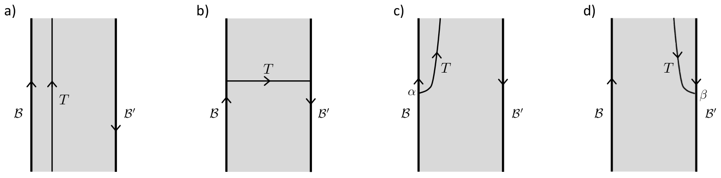
In the analytic approach to geometric Langlands [8, 9], Hecke operators becomes ordinary operators acting on a Hilbert space of quantum states, rather than more abstract functors acting on a category. Not surprisingly, the gauge theory interpretation of Hecke operators in this sense is based on the same ’t Hooft line operators as before, used somewhat differently. In fig. 3(b), we consider the same line operator as before, but now running from left to right of the figure. Some additional data must be supplied at the left and right endpoints where the line operator terminates on a boundary of the strip. Let us assume for the moment that this has been done. Then the line operator becomes an ordinary operator acting on quantum states. Reading the figure from bottom to top, an element of enters at the bottom and after the action of the line operator, a possibly different element of emerges at the top. (If we read the figure from top to bottom, we see the transpose operator acting on the dual vector space .) It is because line operators that are supported on a one-manifold in space at a fixed time can act in this way as ordinary quantum operators that they are traditionally1515 15 In traditional applications in particle physics, there are no boundaries and the support of the line operator is taken to be a closed loop. The operator is then often called a loop operator. called line “operators.”
The purpose of figs. 3(c,d) is to explain what is happening where the line operator of fig. 3(b) ends on the left or right boundary. In fig. 3(c), we see that the left endpoint of the line operator corresponds to an element , and in fig. 3(d), we see that the right endpoint corresponds to an element . Algebraically, the operator associated to a line operator with the additional data can be described as follows. For , we have . Then using the fact that line operators form an algebra and that the trivial line operator appears in the product , we get a map . Finally . This sequence of algebraic manipulations corresponds to the picture of fig. 4. We will sometimes write or for the operator on that is constructed from a line operator or with endpoint data .
We will be particularly interested in elements which originate from local endpoints of a four-dimensional line defect onto four-dimensional boundary conditions which lift and . As remarked in Section 2.1, the four-dimensional lifts of the boundary conditions we are considering are not topological. Instead, they are respectively holomorphic-topological and antiholomorphic-topological. As a consequence, the local endpoint lifting will depend holomorphically on while the local endpoint lifting will depend antiholomorphically on . Notice that the actual path of the line defect in four-dimensions is immaterial, as long as it is topologically equivalent to a straight path. Only the positions of the endpoints in matter.
One of the main properties of ’t Hooft or Hecke operators, when regarded as in [8, 9] as operators on quantum states, is that they commute with each other and with the quantized Hitchin Hamiltonians. This follows from the same reasoning that we used to show that the Hitchin Hamiltonians commute with each other. An ’t Hooft operator commutes with a Hitchin Hamiltonian because one can assume that the support of is disjoint from the point , so that one can slide and up and down past each other (fig. 5(a)) without singularity. Likewise, for distinct points , ’t Hooft operators and commute (fig. 5(b)). Taking the limit , it follows that and commute as well, even for .
4.2 Wilson Operators And Their Eigenvalues
Since the ’t Hooft operators commute with the Hitchin Hamiltonians, they can be diagonalized in the same basis, namely the basis of states , where (Section 3.2). In fact, we can use electric-magnetic duality to determine the eigenvalues of the ’t Hooft operators. An ’t Hooft operator is dual to a Wilson operator , labeled by the same representation of and supported at the same point . While the ’t Hooft operator is a “disorder” operator, whose microscopic definition involves a certain sort of singularity, Wilson operators are defined classically in terms of holonomy, as follows. In the relevant gauge theory on a four-manifold (for our purposes, ), one has a bundle , with connection , to which we can associate a vector bundle . We denote the induced connection on this bundle simply as . The Wilson operator is constructed from the holonomy of the connection on , integrated in general along some oriented path . If is a closed loop, we take the trace of the holonomy around , and this gives a version of the Wilson operator that is important in many physical applications.
However, to compute the eigenvalues of an operator defined by an ’t Hooft line operator that stretches across the strip (fig. 3(b)), we need to consider a dual Wilson operator that similarly stretches across the strip (fig. 6). This is a Wilson operator supported, not on a closed loop, but on a path from on the left boundary of the strip to on the right boundary.
In this case, the holonomy is best understood as a linear transformation from the fiber at to the fiber of this bundle at . Thus with an obvious notation for these fibers, is a linear transformation
| (4.1) |
In order to treat the left and right edges of the strip more symmetrically, it is convenient to introduce the representation dual to and view as a linear function on a representation. Then we have
| (4.2) |
So far, we have a linear function on a vector space, rather than a complex-valued function of connections, which could be quantized to get a quantum operator. To get a complex-valued function of connections, we need to supply vectors , . Then is a complex valued function that can be quantized to get an operator.
A natural construction of suitable vectors was described in Section 2.6. In eqn. (2.15), we described, for a holomorphic oper with associated bundle , a “highest weight section” . Thus, if we are given a vector , then we can define . Similarly, if is an antiholomorphic oper, we have , and hence, for , we have . Note that a dual pair of representations have the same value of .
In the case of a bundle that is a holomorphic oper on the left boundary and an antiholomorphic oper on the right boundary, we can apply the holomorphic version of this construction on the left boundary and the antiholomorphic version on the right boundary, to get
| (4.3) |
This finally is a complex-valued function of connections that can be quantized to get a Wilson operator on physical states. We will call this operator . In the notation, we make use of the fact that the right hand side of eqn. (4.3) depends on and only in the combination . Hopefully it will cause no serious confusion that we use the same notation for a classical holonomy (or its matrix element) and the corresponding quantum operator.
Because of the way the -model localizes on flat connections, it is trivial to diagonalize this operator. The flat connections that satisfy the boundary conditions, with trivializations of the center on the boundary and modulo gauge transformations, are in one-to-one correspondence with the usual basis of states , that diagonalize the Hitchin Hamiltonians. The Wilson operators are diagonal in this basis. The eigenvalue of the quantum operator on a given basis vector is just the value of the corresponding classical function on the classical solution corresponding to . That value is simply the natural dual pairing of the vectors and in the dual vector spaces and . This is true because a flat connection on is actually a pullback from .
The center acts on the physical Hilbert space by (Section 2.8). This transforms the eigenvalue of by a root of unity, which is simply the value of the central element in the representation . For example, if and is the -dimensional representation, eigenvectors of come in -plets of the form , , . This is dual to the fact that on the -model side, the Higgs bundle moduli space has components labeled by a characteristic class . For , there are components, which are cyclically permuted by the ’t Hooft operator dual to , leading to the same structure of the spectrum. In general, the action of on mirrors the way permutes the components of the moduli space.
The holomorphic and antiholomorphic corner data needed to define the operators has consisted precisely of the vectors , . For the -dimensional representation of , we have . We expect the same data to be needed to define holomorphic and antiholomorphic corner data for the dual ’t Hooft operators.
These are arguably the simplest Wilson operators and we will call them principal Wilson operators. However, if the representation is reducible when restricted to a principal subalgebra of , then it is possible to use the more general objects (eqn. (2.14)). So picking , (where and can be chosen independently), we can define , which can again be interpreted as a quantum mechanical operator. Even more generally, we can consider holomorphic and antiholomorphic derivatives with respect to of . It is enough to consider holomorphic derivatives and antiholomorphic ones; this suffices to define a complete set of Wilson operators, since it amounts to applying the linear form (eqn. (4.2)) to a set of vectors that according to the analysis in Section 2.6 form a basis of the finite-dimensional vector space on which is acting.
What happens if we continue to differentiate? With holomorphic derivatives or antiholomorphic ones, we will run into differential equations satisfied by the Wilson operators . The holomorphic and antiholomorphic sections and that were used to define these Wilson operators obey certain holomorphic and antiholomorphic differential equations (Section 2.6 and Appendix C) as a function of , and the corresponding Wilson operators obey the same equations.
Having defined operators that act on the physical Hilbert space , it is natural to ask what algebra they obey. In bulk, the product of line operators mimics the tensor product of representations of . Thus, if , with vector spaces , then the corresponding decomposition of parallel Wilson operators is . This is the appropriate relation for Wilson operators understood as functors acting on boundary conditions, as illustrated in fig. 3(a). From this algebra, the structure of the nonabelian group can be reconstructed, in principle. However, for Wilson operators as operators on quantum states, as we are discussing here, the picture is different. Matters are simplest if we multiply two principal Wilson operators, associated to highest weight vectors in the corresponding representations. Since the tensor product of highest weight vectors in two representations and is a highest weight vector in the tensor product , the product of two principal Wilson line operators is another principal Wilson line operator, for a representation whose highest weight is the sum of the highest weights of and . We will see the structure of the nonabelian group if we multiply the more general Wilson operators and their derivatives.
A dual ’t Hooft operator defined using the -dual data will, of course, have the same eigenvalues as the Wilson operators. The main challenge is to identify precisely the appropriate -model endpoints. We turn to that problem in Section 4.3.
We conclude this discussion of Wilson operators with the following remark. The most illuminating realization of the oper boundary condition in four-dimensional gauge theory involves the Nahm pole [31]. Compared to a more direct approach that was assumed earlier [3] (in which the boundary condition is defined by just specifying the or part of along the boundary), the Nahm pole description of the oper boundary condition has two advantages: it leads directly to the local constraints discussed in Section 2.6; and it also leads to a simple explanation of the duality with the -model description via . If one uses the Nahm pole description of the oper boundary condition, then the complex connection is singular along the boundary, and some renormalization is involved in defining the classical holonomy across the strip and the corresponding quantum operator. The renormalization amounts to a complex gauge transformation that removes the Nahm pole singularity.
4.3 The Dual ’t Hooft Operators
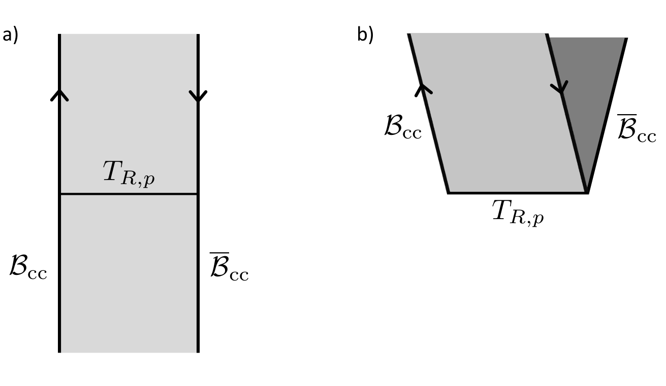
4.3.1 ’t Hooft Operators and Hecke Modifications
An ’t Hooft operator (fig. 7(a)) will produce a jump in the fields and in the associated Higgs bundle , in the sense that the Higgs bundle just below the ’t Hooft operator is generically not isomorphic to the Higgs bundle just above it. They differ by what is known as a Hecke modification. The type of Hecke modification is determined by the magnetic singularity of the ’t Hooft operator, which is classified by a choice of irreducible representation of the dual group . Hecke modifications of bundles and Higgs bundles were described for physicists in [3] and in more detail in Section 4 of [35]. Here we will give a very brief synopsis.
A Hecke modification of a holomorphic bundle at a point is a new bundle that is presented with an isomorphism to away from , but such that this isomorphism does not extend over . A section of is a section of that is allowed to have poles of a specified type at , or that is constrained so that some components have zeroes of a specified type, or both.
For example, if is a rank 2 holomorphic vector bundle, trivialized near so that a section of is a pair of holomorphic functions , then an example of a Hecke modification of at is a new bundle whose sections are a pair , where is holomorphic at but is allowed to have a simple pole at . This example can be slightly generalized to give a family of Hecke modifications of at that are parametrized by . We simply pick a pair of complex numbers , not both zero, representing a point in , and allow a section of to have a polar part proportional to this pair:
| (4.4) |
where is a local parameter at .
The relation between and is reciprocal: instead of saying that we obtain from by allowing a pole of a certain type, we could say that we obtain from by requiring a certain type of zero. If an ’t Hooft operator can map to , then the dual ’t Hooft operator (which is associated to the dual representation) can map to .
A Hecke modification of a Higgs bundle actually does “nothing” to . This means the following. A Hecke modification of is just a Hecke modification of such that is holomorphic as a map . In the example of the rank 2 bundle, the Higgs field is locally , where is a matrix of holomorphic functions. For to be holomorphic as a map , the necessary and sufficient condition is that, if is a section of as characterized in eqn. (4.4), then the polar part of should be a multiple of ; in other words, must be an eigenvector of the matrix . Generically, this condition is not satisfied and hence most Hecke modifications of are not valid as Hecke modifications of . If is not nilpotent, it has two distinct eigenvectors and the Higgs bundle has two possible Hecke modifications of this type at the point ; if is nilpotent but not zero, it has only one eigenvector and there is just one possible Hecke modification of this type; only if does has the same family of possible Hecke modifications of this type at that would have by itself.
Hecke modifications of the type just described can be viewed in two different ways. They are dual to the two-dimensional representation of . This group is self-dual, so the discussion is applicable in gauge theory of . Alternatively, the same Hecke modification is dual to the two-dimensional representation of . In this case, the dual group is . In this application, since the rank two bundles and do not have structure group, the preceding discussion should be restated in terms of the corresponding adjoint bundles and
In this example, let be the eigenvalue of acting on :
| (4.5) |
As we vary the choice of and , varies holomorphically. It defines a holomorphic function on the space of Hecke modifications of this type. Since the eigenvalues of are , we have
| (4.6) |
where is a linear combination of the Hitchin Hamiltonians. The sign of distinguishes the two choices of Hecke modifications compatible with a given Higgs field.
4.3.2 Hecke Correspondences
The ’t Hooft operator can be viewed as an interface between the -model of and itself. This is a tautology; in fig. 7(a), we see the -model of above and below , so we can view as an interface between two copies of this -model. In fact, this interface is of type , because of the supersymmetric properties of . It is convenient to use a folding trick similar to the one of fig. 1. Instead of associating to an interface in the -model of , we can associate to it a brane or boundary condition of type in the -model of a product (fig. 7(b)). Here the symplectic structure of is , with a minus sign in one factor because folding reverses the sign of the symplectic structure.
Let us consider explicitly what will look like for the basic example, described in Section 4.3.1, that is the two-dimensional representation of . What is its complex dimension? If has genus , then the choice of a bundle depends on complex parameters. Choosing ’s that can be made from by action of adds one more complex parameter. But we have to constrain the Higgs field so that is an eigenvector of . So the choice of involves parameters, not . The upshot is that the support of has dimension , and thus is middle-dimensional in . Because is middle-dimensional and is the support of a brane of type , it must be a complex Lagrangian submanifold. The brane has rank 1 because the Hecke transformation by which produces from is generically unique, if it exists. In short, is a rank 1 Lagrangian brane of type .
We can be more specific, because is manifestly invariant under scaling of , which corresponds to the symmetry of . We can give a simple description in the same sense in which can be approximated by its dense open set . (As in the general discussion of quantization, we expect that this approximation is sufficient in an theory.) The intersection of with is the variety that parametrizes pairs such that can be reached from by a Hecke transformation of type at the point . invariance of means that it can identified as the conormal bundle1616 16 If a submanifold is defined locally by vanishing of some coordinates , then its conormal bundle in is defined by setting to zero those coordinates and the momenta that Poisson-commute with them. of . is called the Hecke correspondence in this situation, and is the Hecke correspondence for Higgs bundles.
The particular example of an ’t Hooft operator dual to the two-dimensional representation of is relatively simple because the space of possible Hecke modifications of a given bundle at a given point is 1-dimensional. In general, the space of Hecke modifications of that can be made at by has a dimension that depends on and becomes arbitrarily large if is a representation of of large highest weight. When the dimension is sufficiently large, every can be made from by and the ways to do so form a complex manifold of positive dimension. In such a situation, is rather complicated. It has a component on which the Higgs field vanishes (if is produced from by a generic Hecke modification of very high weight, then no nonzero is holomorphic as a map ), and other components with nonzero Higgs field (it is possible to pick a Hecke modification of of arbitrarily high weight such that is holomorphic). The bundle of restricted to the various components is not just of rank 1. For example, restricted to the component on which the Higgs field vanishes, this bundle is formally (that is, modulo a proper treatment of singularities), the cohomology of .
4.3.3 ’t Hooft Line Operators as Operators on Quantum States
Under fairly general conditions, if a symplectic manifold can be quantized by branes to get a Hilbert space , an -brane in (with additional data at the “corners,” as discussed presently) can be interpreted as a quantum operator on . This is discussed in general in Section 4 of [22]. In general it is difficult to get an explicit description of such an operator. But here we are in a special situation with a simple answer. That is because is effectively a cotangent bundle , and the brane of interest is supported on the conormal bundle of a subvariety .
A fairly general operator acting on the quantization of can be represented by an integral kernel which is a half-density on , The action of on a state is
| (4.7) |
What sort of integral kernel should we expect for the quantum operator associated to the ’t Hooft operator ? The points and in eqn. (4.7) correspond in fig. 7(a) to the fields just below and just above the line operator . So they correspond to bundles , such that can be reached from by a Hecke modification of type at . Hence in a classical limit, is a distribution supported on , which parametrizes such pairs . The simplest case, which we will consider first, is that is a delta function in the directions normal to . More generally, in its dependence on the normal directions, can be proportional to arbitrary derivatives of a delta function in the normal variables.
In general, one would expect quantum corrections to the claim that is supported on the underlying classical correspondence . However, in the present situation, there are no corrections, because the symplectic manifold that is being quantized is a cotangent bundle , and the correspondence is a conormal bundle in . The scale invariance of the cotangent bundle and the conormal bundle imply that the kernel cannot depend on and can be evaluated in a semiclassical limit.
We should add a note on why it is valid here to argue based on scaling symmetry. Brane quantization is based, as always, on studying in the context of a suitable complexification. Similarly to study in brane quantization involves complexifying it in a complexification of . A scaling argument in brane quantization really involves scaling of the complexifications. Such an argument is valid in the present setting because the structure of as a cotangent bundle and of as a conormal bundle do extend to holomorphic stuctures of the same type for their complexifications.
We should also clarify what we mean by “semiclassical limit.” A one-loop correction is built into the assertion that a wavefunction is a half-density rather than a function and that is correspondingly a half-density on . The assertion that can be computed semiclassically means that there is no quantum correction beyond this fact.
According to Etingof, Frenkel, and Kazhdan [9], the Hecke operator dual to the two-dimensional representation of is defined by an integral kernel that can be factored as the product of holomorphic and antiholomorphic factors. Such a holomorphic factorization is expected in the -model. A holomorphic factor will come from the left endpoint of in fig. 7(a), or equivalently the lower left corner in fig. 7(b), and an antiholomorphic factor will come from the right endpoint or the lower right corner. We view the ’t Hooft operator as a rank 1 brane of type in , with trivial bundle. In general, the space of corners between a brane of this type, supported on a Lagrangian submanifold , and the canonical coisotropic -brane is . The ’t Hooft operator corresponds to a brane whose support is the Hecke correspondence . So in this case, a holomorphic corner is a holomorphic section . Similarly, an antiholomorphic corner is an element , where is with opposite complex structure.
The product of and will be a half-density on . We will show that this data is precisely what is needed to define a distributional kernel . If and are pull-backs from , we will get a delta function kernel. If they have a polynomial dependence on the fiber of , we will get a linear combination of derivatives of a delta function.
In order to describe a delta function distribution, we pick some local coordinates. We parametrize the input to the Hecke transformation by coordinates on . We will write for the half-density , and similarly for other variables introduced momentarily. For a given , the output of the Hecke transformation ranges over a copy of that we will call ; we parametrize it by a complex variable . is of complex codimension in . can be defined locally by a condition , where are local holomorphic coordinates on the normal bundle to in . We can write the kernel as
| (4.8) |
where and the delta function is defined by . In view of that last relation, the delta function transforms under a change of coordinates on the normal bundle as , which means that the possible kernels are in one-to-one correspondence with objects
| (4.9) |
The Hecke correspondence for Higgs bundles is parametrized locally by the coordinates and , introduced above, which parametrize the Hecke correspondence for bundles, and additional variables that parametrize the choice of Higgs field. Since is the conormal bundle of , the variables are dual to the normal bundle coordinates that appear in eqn. (4.8). Therefore, we can replace with , and the possible delta function kernels are in one-to-one correspondence with half-densities
| (4.10) |
on such that is independent of .
This discussion is immediately generalized to linear combinations of normal derivatives of a delta function. A kernel that involves normal derivatives of a delta function
| (4.11) |
corresponds to a half-density
| (4.12) |
on such that depends polynomially on .
A holomorphically factorized kernel will take the form where and are respectively holomorphic and antiholomorphic. We can now see what kind of holomorphic object must be. must be a half-density on the Hecke correspondence in the holomorphic sense: . In more standard language, must be an element of . As explained earlier, this is the expected form of the answer in the -model for a left endpoint of . Similarly, is an antiholomorphic section of the anticanonical bundle of , again in accord with the -model expectation.
If and only if is a Calabi-Yau manifold, there is a particular holomorphic section of that is everywhere nonzero. If such a exists, then the data that defines any other holomorphic corner is , where is a holomorphic function on . In particular, such a function (with only polynomial growth) is a polynomial in the Hitchin Hamiltonians and the holomorphic function that was defined in eqn. (4.5), up to the relation , which expresses as a linear combination of the . A nonconstant polynomial has nontrivial zeroes, so is everywhere nonzero only if is a constant, showing that is unique, up to a constant multiple, if it exists.1717 17 More generally, if is a complex manifold with , then an everywhere nonzero holomorphic function on , with no exponential growth, is constant. Indeed, since , the closed 1-form is exact, for some , so (with a nonzero constant ) and has exponential growth unless it is constant. The Hecke correspondence for -bundles satisfies . The Hecke correspondence for Higgs bundles is the conormal bundle of and hence . Corners of the form , where is a polynomial in the Hitchin Hamiltonians and , precisely match the corners for Wilson lines, built from , and polynomials in the observables dual to the Hitchin Hamiltonians.
Such a does indeed exist, by virtue of a result of Beilinson and Drinfeld [1] that was important in the work of Etingof, Frenkel, and Kazhdan [9]. The properties of mirror those of the simplest Wilson line corner of Section 4.2. In particular, according to the result of Beilinson and Drinfeld, , like , varies with as a section of . Of course, the existence of such a mirror of is expected from electric-magnetic duality.
A slightly different formulation was useful in [9]. To explain this, let us go back to eqn. (4.9), from which we see that if can be holomorphically factorized, then the holomorphic factor is a holomorphic form . We can replace with where parametrizes the output of the Hecke transformation. So in other words a holomorphically factorized kernel will come from a holomorphic object1818 18 Since is determined by and , and reciprocally is determined by and , we could equally well write instead of .
| (4.13) |
If we multiply by its complex conjugate, we get
| (4.14) |
This leads directly to the definition used in [9]. The quantity can be regarded as a map from half-densities in to half-densities in , valued in differential forms that can be integrated over . That integral gives the Hecke operator at the point :
| (4.15) |
In Section 8, we will interpret some of these statements via two-dimensional chiral algebras. In particular, the considerations about adjoint-valued chiral fermions in Section 8.3 are a physicist’s interpretation of the original analysis of Beilinson and Drinfeld. The chiral algebra approach is local on and and can potentially be extended to situations where the space of Hecke modifications relating two given bundles has positive dimension.
4.3.4 The Affine Grassmannian
So far, we have considered the simplest examples of Hecke modifications. But to develop the theory further, one wants a more systematic approach.
As motivation, we consider first the case of a holomorphic vector bundle of rank . Let be a local holomorphic parameter that vanishes at a point . Let be a small neighborhood of . has an open cover with two open sets, namely and ( with removed). Pick a trivialization of in a small neighborhood of the point and restrict to . Let be a trivial rank vector bundle. We have an open cover of by open sets with vector bundles and . So we can define a new vector bundle by gluing together and over via a gauge transformation. For example, we can use the diagonal gauge transformation from to
| (4.16) |
with integers . For , with suitable choices of the , this gives an example of a Hecke modification of a -bundle dual to an arbitrary irreducible finite-dimensional representation of . For , one modifies this by requiring so that is valued in , and for , one considers the to be valued in , with (this is equivalent to saying that if is written in a representation of , then only integer powers of appear). A constant shift of all by , where (or for ) does not affect the space of Hecke modifications, since one can compensate for it by .
For any , one can make a similar construction replacing diagonal matrices whose entries are powers of with a homomorphism where is the punctured -plane, is a complex maximal torus of , and , which generalizes the -plet of integers in the previous paragraph, is an integral weight of the dual group , corresponding physically to the magnetic charge of an ’t Hooft operator.
What we have described so far is a standard example of a Hecke transformation dual to an arbitrary finite-dimensional representation of ; is encoded in the integers or the choice of . This construction depended on the initial choice of a trivialization of over . By varying the choice of trivialization, one can obtain a whole space of Hecke modifications of the same type. Once we pick a reference trivialization, any other trivialization of over the set would be obtained from the reference one by applying some gauge transformation that is holomorphic in . The standard Hecke modification associated to this alternative trivialization of is described in the reference trivialization by the modified singular gauge transformation .
Two singular gauge transformations lead to the same if they can be related by composition from the right with a gauge transformation defined on . Two trivializations of will thus give the same standard Hecke modification if the corresponding gauge transformations and satisfy
| (4.17) |
for some .
These relations can be formalized with the help of the affine Grassmannian . It is customary to denote as the (infinite-dimensional) space of -valued gauge transformations defined on and as the subspace of such gauge transformations which extend holomorphically to . The affine Grassmannian
| (4.18) |
parameterizes equivalent singular gauge transformations. We define to be the orbit in of the standard Hecke modification by the gluing function :
| (4.19) |
Every point in is on such an orbit, for some .
For generic choices of and , one runs into a phenomenon of “monopole bubbling” in which a downward jump can occur in the magnetic charge of an ’t Hooft or Hecke operator (this was introduced in [36, 37]; see Section 10.2 of [3] for a short introduction). Essentially, the orbit is not closed in the affine Grassmannian, and the (possibly singular) closure of the orbit includes other orbits with smaller charge. This can considerably complicate the analysis.
For or a related group or , the condition to avoid monopole bubbling is that for all . Up to a constant shift of all the (which does not affect the space of Hecke modifications, as explained in the discussion of eqn. (4.16)), to avoid monopole bubbling we can assume that of the are and the others 0. Explicitly, this corresponds to a Hecke modification of the following sort. For a rank holomorphic vector bundle and , one chooses a -dimensional subspace and defines a new vector bundle whose sections are sections of that are allowed to have a simple pole at with residue in . The space of Hecke modifications of this type is parametrized by the choice of , that is, by the Grassmannian of -dimensional subspaces of . Such Hecke modifications are dual to the antisymmetric power of the fundamental representation of or . In this situation, will act as a matrix on the polar part of . The characteristic polynomial of the restriction of takes the general form , for some holomorphic functions . These functions satisfy polynomial relationships with the Hitchin Hamiltonians which encode the constraint that divides the characteristic polynomial of .
5 Quantum-Deformed WKB Condition
5.1 Quantum States And The Hitchin Fibration
A slightly different way to think about an eigenfunction of the Wilson operators and the Hitchin Hamiltonians is as follows. Let be a point in corresponding to a flat bundle , and let be a -brane supported at , with a rank 1 (and inevitably trivial) bundle. Then the part of of degree zero1919 19 The -model has a conserved fermion number symmetry, with the differential having fermion number or degree 1. When , is also nonzero in positive degrees, but the positive degree states do not contribute in this discussion because is entirely in degree 0. A similar remark applies later when we discuss the -model. is a copy of if , that is if is a holomorphic oper. Otherwise . Similarly, the degree 0 part of is if , that is if is an antiholomorphic oper, and otherwise zero. If and only if is both an oper and an anti-oper, we can pick nonzero elements , , and then define the element . A picture representing this situation is fig. 8(a). The brane is used to provide a boundary condition at the bottom of the strip; and provide the “corner data” needed to define boundary conditions at the corners of the picture. The path integral with the “initial conditions” set by defines a physical state of the system. This state is the desired eigenstate of the Hitchin Hamiltonians and the Wilson operators.
Via electric-magnetic duality, we can get a dual picture. After compactification on an oriented two-manifold , electric-magnetic duality of super Yang-Mills theory reduces at low energies to a mirror symmetry of the Higgs bundle moduli space [26, 27]. As explained in [38], this is a rare instance in which the SYZ interpretation [39] of mirror symmetry as -duality on the fibers of a family of Lagrangian tori can be made very explicit. The Hitchin fibration is the map that takes a Higgs bundle to the characteristic poiynomial of . The fibers of the map are abelian varieties that are complex Lagrangian submanifolds in complex structure . This in particular means that they are Lagrangian submanifolds from the point of view of the real symplectic structure of the Higgs bundle moduli space. Hence, in the -model with symplectic structure , the Hitchin fibration can be viewed as an SYZ fibration by Lagrangian submanifolds that generically are tori. -duality on the fibers of this fibration maps the -model of symplectic structure to the -model of complex structure . The relation of electric-magnetic duality to this instance of mirror symmetry was an important input in [3].
In particular, mirror symmetry in this situation maps a rank 1 brane supported at a point to a brane supported on a fiber of the Hitchin fibration, with a bundle that is a flat line bundle2020 20 In general, the bundle of a rank 1 brane is more canonically a structure rather than a line bundle. In the present context, as is an abelian variety and so has a canonical spin structure, the distinction is not important. . The duals of and are elements and . The element , which corresponds to the picture of fig. 8(b), represents an element of in the magnetic description, in which the Hitchin Hamiltonians are differential operators acting on half-densities on and Wilson operators are replaced by ’t Hooft operators.
The branes and both have compact support, consisting of either a point or a fiber of the Hitchin fibration. Compact support makes it manifest that the states created by these branes (plus corner data) are normalizable. More than that, compact support means that these states have well-defined pairings with states that are constructed similarly using an arbitrary brane , possibly with noncompact support, again with suitable corner data. In other words, the pairing constructed from the rectangle of fig. 8(c) is always well-defined, regardless of the brane at the top of the rectangle, as long as the brane at the bottom of the rectangle has compact support. This means roughly that an arbitrary brane, with a choice of corner data, defines a distributional state, not necessarily a normalizable vector in the Hilbert space , while a brane of compact support defines a vector that can be paired with any distribution. The Hilbert space is contained in the space of distributional states, and contains a subspace, roughly analogous to a Schwartz space, spanned by states associated to branes of compact support. The eigenfunctions of the Hitchin Hamiltonians lie in this subspace.
The -model gives a clear answer to the question of which points are associated to physical states: these are points in . It is more difficult to extract directly from the -model a prediction for which pairs are similarly associated to physical states. We will only be able to get a sort of semiclassical answer, which we expect to be valid asymptotically, in a sense that will be explained.
We recall that the bundles of the branes and are dual line bundles and , and that the prequantum line bundle of , in the sense of geometric quantization, is . We want the condition on and such that corners and exist.
We will describe the condition for and to exist to lowest order in -model perturbation theory, and we will also explain to what extent higher order corrections can or cannot change the picture, in the regime where they are small. So let us first explain the regime in which -model perturbation theory is valid. This is the case that the Higgs field is parametrically large and far away from the discriminant locus (on which the spectral curve becomes singular). Concretely if is any Higgs bundle with a smooth spectral curve, and we rescale by a large factor
| (5.1) |
with any fixed value of , then -model perturbation theory becomes valid. For , the Higgs bundle moduli space has a concrete “semi-flat” description [40], leading to semiclassical results and asymptotic expansions as for a variety of questions, including what we will consider here. We will call the region the WKB limit, for reasons that will emerge.
The brane is of type . For such a brane, with support and bundle , the leading -model approximation to , where has bundle , is the cohomology of with values in2121 21 As remarked in footnote 20, and likewise is canonically a structure on , not a line bundle. Likewise, is not canonically defined as a line bundle (and for general may not exist at all as a line bundle) but on any complex manifold, is canonically defined as a structure. Hence the product exists canonically as an ordinary line bundle and the answer stated in the text makes sense. In our application, is trivial, and we can likewise take to be trivial and define as a line bundle. , where is a square root of the canonical bundle of (see Appendix B of [22]). This comes about because the leading -model approximation to the -model differential is
| (5.2) |
where is a -form on that defines the complex structure of the line bundle . The line bundle is flat when restricted to , because is a complex Lagrangian submanifold. The line bundle is flat, because it is the bundle of a Lagrangian brane. And as is a complex torus, we can take to be trivial and omit this factor. The cohomology of a complex torus with values in a flat line bundle vanishes unless this line bundle is trivial. So in the leading -model approximation, vanishes unless we pick . For ,we can pick a nonzero .
Similarly, as the bundle of is , the leading -model approximation to is the cohomology of with values in , or, taking to be trivial, just . This cohomology vanishes if is nontrivial; if it is trivial, which is so precisely if , we can choose a nonzero .
In short, we can use the brane with suitable corner data to define a state in if and only if we can choose to be isomorphic to both and . In other words, the condition is that must be trivial. As the prequantum line bundle over is , the condition is that must be trivial when restricted to .
This is actually the WKB condition of elementary quantum mechanics, which also is part of the theory of geometric quantization. To put the condition in a more familiar form, recall that the symplectic form of is cohomologically trivial, so it can be written as for a 1-form . The prequantum line bundle is supposed to be a unitary line bundle with a connection of curvature . We can take to be a trivial line bundle with the connection . is flat when restricted to because is a Lagrangian submanifold. The condition that is trivial is that its global holonomies vanish. In other words, the condition is that if is a 1-cycle, then the holonomy of around must vanish: or in other words . To put this condition in a perhaps more familiar form, we can approximate as a cotangent bundle and choose , where are coordinates on the base of the cotangent bundle and are fiber coordinates. Then the condition is that
| (5.3) |
which may be recognizable as the WKB condition for associating a quantum state to the Lagrangian submanifold .
We have reached this conclusion to lowest order in -model (or gauge theory) perturbation theory, and we do not claim that the result is exact. However, it is possible to argue that, at least sufficiently near the WKB limit, there is a quantum-corrected WKB condition that leads to qualitatively similar results. Consider correcting the computation of or in perturbation theory in inverse powers of the parameter that was introduced in eqn. (5.1). This has the effect of shifting the -form by a -form , leading to
| (5.4) |
Whatever the are, we can compensate for them by shifting . An arbitrary shift in can be interpreted as the sum of a -exact term, which does not affect the cohomology of , plus a term that can be interpreted as resulting from a shift in the line bundle . Thus, instead of needing and to be trivial in order to associate a quantum state with , we need to satisfy conditions that are asymptotically close to these. Correspondingly, the classical WKB condition for to be trivial is modified, at least for sufficiently large , to a quantum WKB condition that determines which fibers of the Hitchin fibration are associated to quantum states.
5.2 WKB Condition and Special Geometry
In order to better understand the quantization condition, it is useful to recall some facts about the special geometry which governs the structure of , as well as complex integrable systems that arise in Seiberg-Witten theory [41, 42, 43, 44, 45]. The basic ingredients of the geometry are
- •
The base of the Hitchin fibration, of complex dimension . We denote a point in the base as and the discriminant locus as .
- •
A local system of lattices of rank defined over ( with removed), equipped with a symplectic form .2222 22 In a true Seiberg-Witten geometry the symplectic form is integer-valued and is self-dual. The Seiberg-Witten geometry is self-mirror. Hitchin systems are related to Seiberg-Witten geometries by discrete orbifold operations which relax these conditions. We will denote a charge (an element of ) as .
- •
A collection of central charges which vary holomorphically on . We will denote the central charge evaluated on a charge as . The are also identified with periods of the canonical 1-form on the spectral curve of the Hitchin system.
- •
Real angular coordinates on the fibers of the complex integrable system. We will denote the coordinates evaluated on a charge as . They are dual to the under the complex Poisson bracket
(5.5)
The complex symplectic form in complex structure is defined with the help of the inverse pairing:
| (5.6) |
Correspondingly, we have a 1-form
| (5.7) |
satisfying , with periods .
We will use this special coordinate system for . The parameters specify a fiber of the Hitchin fibration, which is an abelian variety, and the angles parameterize the choice of a flat line bundle . The WKB conditions for the existence of corners are thus that and the quantization condition becomes .
The branes as -branes are supposed to depend on the data holomorphically in complex structure , as the twist on is mirror to the twist on . Writing functions of which are holomorphic in complex structure is essentially as challenging as computing the hyper-Kähler metric on the moduli space. In the WKB region, though, the functions
| (5.8) |
are an excellent “semiflat” approximation to -holomorphic functions. The Cauchy-Riemann equations fail by corrections suppressed exponentially in the WKB region [45].2323 23 One can define locally some corrected which are truly -holomorphic, but non-trivial “wall crossing” coordinate transformations are required in different patches [40]. This subtlety will not be important here. These statements have a transparent -model interpretation. The semiclassical -brane moduli combine the data with the deformation data associated to the same 1-forms on the brane support to give the coordinates . The only corrections are non-perturbative and due to disk instantons ending on a cycle . These only exist at codimension one loci where is real and lead to the wall-crossing transformations. The complex symplectic form in complex structure is approximately
| (5.9) |
Stated in this language, the WKB condition for the existence of a corner becomes
| (5.10) |
This can be interpreted as the parametric definition of an -dimensional complex Lagrangian submanifold, as expected. Surprisingly, the parameters coincide with the coordinates on and thus we get an approximate holomorphic identification between and the space of branes equipped with a corner.
This identification is only valid in a semiclassical approximation. To make such an expansion, as in Section 5.1, we replace with , and take to be large. The corner condition receives perturbative corrections, which will take a systematic form
| (5.11) |
We introduced parameters that cannot be taken to coincide with the coordinates that are holomorphic in complex structure . The relation between the two follows from the comparison of (5.10) and (5.8):
| (5.12) |
The perturbatively-corrected quantization condition to have both types of corners will become
| (5.13) |
5.3 Match with real WKB opers
There is another natural occurrence of the periods of the canonical 1-form on the spectral curve. If we attempt a WKB analysis on of the oper differential equation, the monodromy data of the oper flat connection will be computed at the leading order in terms of the exponentiated periods [46, 47, 48, 49, 50]. Here we employed a non-canonical identification between and . For example, for we would write the oper differential operator as a reference operator deformed by a large quadratic differential
| (5.14) |
and the leading WKB approximation would involve the periods of the WKB 1-form . Here is the classical stress tensor, a reference choice of classical stress tensor and is the scaling parameter.
The WKB calculation is really a combination of a topological and an analytic problem. The topological problem involves a careful Stokes analysis of the asymptotic behaviour of the flat sections of the connection. The analytic problem involves the computation of the Voros symbols, which are periods of the all-orders WKB 1-form. Remarkably, the Voros symbols precisely compute the corrected coordinates of the oper in the space of flat connections [50]:
| (5.15) |
The WKB analysis of the oper differential equation thus gives directly the -model analogue of the WKB corner condition in the mirror model.
6 Real Bundles
6.1 The Setup
So far we have studied the quantization of as a real symplectic manifold. An alternative is to view as a complex symplectic manifold with complex structure and holomorphic symplectic structure , and quantize a real symplectic submanifold . For this, as explained in Section 2.1, we look for an antiholomorphic involution of that satisfies . In our application, will be a cotangent bundle, leading to a simple description of the Hilbert space and of the action of the Hecke operators, and a real integrable system, equipped with a real version of the Hitchin fibration.
The classification of the possible antiholomorphic involutions is the same whether one considers holomorphic bundles as in [51, 52] or Higgs bundles, as in [53, 54, 55]. Those references provide much more detail than we will explain here. We also note that the three-manifold that we will use in studying the duality was introduced in Section 11 of [53]. That paper also contains a duality proposal based on the structure of as a real integrable system.
A suitable involution of can be constructed starting with an antiholomorphic involution of the Riemann surface , which exists for suitable choices of . An antiholomorphic map reverses the orientation of ; conversely, if is an orientation-reversing smooth involution of an oriented two-manifold , then one can pick a complex structure on such that acts antiholomorphically.2424 24 Pick any Riemannian metric on . Then is a -invariant metric, and acts antiholomorphically in the complex structure determined by . Topologically, the possible choices of can be classified as follows. If has genus , then its Euler characteristic is and the quotient will have Euler characteristic . can be any possibly unorientable two-manifold, possibly with boundary, of Euler characteristic . The boundary of comes from the fixed points of . These fixed points make up a certain number of circles; any integer number of circles from to is possible. For example, if , can be a disc or ; if , can be a cylinder, a Mobius strip, or a Klein bottle. Having fixed , we then choose the topological type of a lift of to act on a smooth -bundle . We choose the lift to preserve . If is a fixed point of , then acts on the fiber of over by an automorphism of . Here can be an inner automorphism, that is, conjugation by an element of , but more generally, if has non-trivial outer automorphisms, may be an outer automorphism. The conjugacy class of is constant on each fixed circle , and we denote it as . The condition places a condition on . Since a Higgs bundle is defined by fields that are adjoint-valued, purely to define an involution of the Higgs bundle moduli space , we require only that in the adjoint form of ; as an element of , might be a central element not equal to 1. The precise condition that should be imposed on depends on topological subtleties that were reviewed in Section 2.7; we will return to this point in Section 6.3. If acts freely and is not simply-connected, other issues come into play in lifting to act on . For example, for , a lift of to act on only exists if . In that case, there are two topologically inequivalent lifts, parametrized by , where is the quotient of by .
A Riemann surface endowed with antiholomorphic involution can be viewed as an algebraic curve defined over . The boundary points of , if any, correspond to the real points of over . Once it has been lifted to act on the smooth bundle , also acts on , the moduli space of flat connections on , and on the corresponding Higgs bundle moduli space . Whether or not there are fixed points in the action of on , there always are fixed points in the action of on2525 25 If is any connection on , then is a -invariant connection. Generically, the part of this connection defines a stable -bundle, which corresponds to a -invariant point in . The same connection with zero Higgs field defines a -invariant point in . and on . Each component of the fixed point set of on or is middle-dimensional. This is a general property of antiholomorphic involutions of complex manifolds.
We will write or for a component of the fixed point set of acting on or , respectively. The components in general are classified by additional data that we have not introduced so far. In particular, viewing or as moduli spaces of flat -valued or -valued connections, the monodromy of a flat bundle around will be invariant under , so it will lie in the -invariant subgroup or of or . and are connected if is simply-connected, but in general not otherwise (for example, if and , then contains the component of the identity and another component that contains the element ). So in general, to specify a component of the fixed point sets requires an additional choice for each .
Associated to each fixed circle is a real form of the complex Lie group . Writing for the antiholomorphic involution of that leaves fixed the compact form , is defined by the condition
| (6.1) |
In case is conjugation by , the condition becomes
| (6.2) |
, with symplectic structure , is the real symplectic manifold that we want to quantize. The definition of has depended on various choices which we are not indicating in the notation, but regardless of those choices, has as a complexification and this complexification has the appropriate properties for brane quantization of . has a real polarization that is defined as follows: a leaf of the polarization consists of -invariant Higgs pairs with fixed , but varying . The same condition, without the requirement of -invariance, defines a holomorphic polarization of the complexification of . Hence brane quantization of is equivalent to its quantization using this real polarization. Concretely, in this real polarization, can be approximated by the cotangent bundle for the same reason that such a statement holds for the full Higgs bundle moduli space: if is a -invariant Higgs bundle representing a point in , then generically represents a cotangent vector to at the point in corresponding to . Therefore, the Hilbert space that arises in quantization of is the space of half-densities on , the usual answer for geometric quantization of a cotangent bundle.
We can also restrict the Hitchin fibration to the -invariant locus. acts on the base of the Hitchin fibration with a fixed point set . Functions on are Poisson-commuting (with respect to the real symplectic structure of ). So is a real integrable system. The generic fiber of the map is a real torus. Baraglia and Schaposnik [53] proposed to define a mirror symmetry between and a similar moduli space with replaced by by -duality on the fibers of the real integrable system. In general, one would expect such a definition to give reliable results at least asymptotically, far from the discriminant locus of the real integrable system. At least when acts freely, one can be more precise, as we discuss next.
6.2 Four-Dimensional Picture And Duality
To learn something interesting about this construction, one wants to apply duality, and for this, as usual, a four-dimensional picture is helpful.
For a four-dimensional picture, we start with the usual four-manifold , where is a strip. Here labels the “time” and is an interval, say the interval . We then modify by imposing an equivalence relation on the right boundary at : we declare that, for , points and are equivalent. (No equivalence is imposed except at .) Imposing this equivalence relation amounts to requiring that the data at should be -invariant (up to a gauge transformation). So this is a way to implement in four dimensions what in the two-dimensional picture of Section 6.1 was the brane at the right boundary. We write for the quotient of by this equivalence relation. It is convenient to factor out the time and define .
There is an alternative construction of as a quotient by the group generated by . For this, we start with a doubled interval . Then we divide by the symmetry that acts by . A fundamental domain is the region , so the quotient is the same as before.
Simplest is the case that acts freely on . is then actually an orientable manifold, whose boundary is a single copy of , at . is the total space of a real line bundle over . itself and the real line bundle are both unorientable, but the total space is orientable.
The four-dimensional picture associated to quantization of is just the -model on , with boundary conditions at . There is no need for an explicit boundary condition at , as there is no boundary there. What in the two-dimensional description was a Lagrangian brane supported on has been absorbed into the geometry of .
Therefore, without further ado we can describe a dual description. The dual is just the -model with gauge group on the same four-manifold , but now with boundary conditions at . In a two-dimensional language, the brane dual to is supported on . In particular, it is supported on the same locus on the base of the Hitchin fibration. This is in accord with the duality proposal of Baraglia and Schaposnik [53], which appears to be valid at least when acts freely on .
As usual, it is relatively easy to describe the physical states of the -model in quantization on and the eigenvalues of the Hitchin Hamiltonians. The first step is localization of the -model on complex-valued flat connections, which here means -valued flat connections on that satisfy the oper boundary condition. To put it differently, the localization is on flat bundles whose restriction to is a holomorphic oper. Let be the set of isomorphism classes of such bundles. For positivity of the Hilbert space inner product, we expect to be a discrete set of nondegenerate points (see Appendix B), similarly to the analogous set encountered in the quantization of the full Higgs bundle moduli space. Assuming this, the Hilbert space has a basis labeled by . The are eigenfunctions of the Hitchin Hamiltonians. The eigenvalue of a Hitchin Hamiltonian on is the value of the corresponding function at the point in that corresponds to the boundary values of the flat bundle associated to .
If an oper bundle over extends over as a flat bundle, then in particular this implies that the antihomomorphic involution lifts to an action on and therefore that is an antiholomorphic oper, as well as a holomorphic one. So the set has a natural map to . However, in general the map from to is not an embedding, since a -invariant flat bundle on the boundary of that is a holomorphic oper may have more than one extension as a flat bundle over the interior of . To analyze this situation, note that flat bundles over correspond to homomorphisms , up to conjugation. As is contractible to , we can equally well consider . The group has an index 2 subgroup consisting of orientation-preserving loops in . Such loops can be deformed to the boundary of , so once a flat bundle is given on the boundary of , the restriction of the corresponding homomorphism to is uniquely determined. However, there is some freedom in the extension of to the rest of . is generated by the index 2 subgroup together with any orientation-reversing element . To complete the description of , we need to specify . is supposed to be a homomorphism, so we require , where, since , is determined by the boundary data. If is a regular element of , then there are only finitely many choices for , but is not uniquely determined. In particular, we are always free to transform , where is an element of order 2 of the center of . Thus the subgroup of the center of consisting of elements of order 2 acts freely on . (For simple , is 1, , or , depending on .)
The -model dual of the action of is the following. Topologically, for simple , a -bundle on the three-manifold is classified by . In the present instance, is contractible to so . As is unorientable, one has , where is the subgroup of consisting of elements of order 2. Thus on the -model side, there is a grading of the Hilbert space by . As , this matches the action in the -model.
Finally let us discuss the natural line operators in this problem. As in Section 4, we could in principle consider Wilson and ’t Hooft line operators supported on an arbitrary 1-manifold . But a natural special case is the following. Pick a point . In , there is a natural path between the points and on the left and right boundaries: we simply set . Upon dividing by the group generated by , descends to a path , between the boundary points and . In a purely two-dimensional description, one would have needed endpoint or corner data associated to the real brane , but in the four-dimensional description, this is not needed as has no endpoint at .
As in Section 4.2, we can choose an arbitrary representation of and consider the holonomy of the bundle on the curve . However, to turn this holonomy into a quantum operator , we need, as before, to supply endpoint data. For example, if we choose canonical endpoints at and at , the Wilson operator will take the form of the inner product between transported to and . As in Section 4.2, the Wilson operators constructed this way are diagonal on the basis of states , with eigenvalues given by evaluating the inner product on the concrete canonical sections in the flat bundle corresponding to .
The duality predicts that a dual ’t Hooft operator associated to the same representation , supported on the same curve , and with -dual endpoints, has the same eigenvalues. The dual ’t Hooft operator is associated to a real Hecke correspondence of with itself; is just the -invariant locus of the ordinary Hecke correspondence of with itself, for a -conjugate pair of points labeled by the conjugate (or dual) pair of representations . As in Section 4.3.3, because of the scaling symmetry of the cotangent bundle, the quantum operator associated to the Hecke correspondence can be defined by a semiclassical formula. Beyond the ingredients that were used in Section 4.3.3, one needs one further fact. Suppose that is a complex manifold with canonical bundle ; let be an antiholomorphic involution with fixed point set , and assume thast is orientable. Then a holomorphic section of restricts on to a complex-valued half-density. Hence a holomorphic endpoint or corner that one would use (together with an antiholomorphic one) in defining an ’t Hooft operator in the quantization of restricts on the real locus to a half-density that defines an ’t Hooft operator in the quantization of . In our application, is orientable because is a Calabi-Yau manifold, as discussed in Section 4.3.3; the Calabi-Yau form of a Calabi-Yau manifold that has a real structure can be chosen to be real and restricts on the real locus to a top-degree differential form that defines an orientation of .
6.3 The Case That Does Not Act Freely
Now we consider the case that does not act freely on . Suppose that the action of leaves fixed a circle . Then contains as a locus of orbifold fixed points. The local behavior near looks like
| (6.3) |
where acts on as a rotation. In the four-manifold , the fixed point set is .
We recall that in general the action on is accompanied by an action of an automorphism that satisfies at least in the adjoint form of . In gauge theory, one might expect to require in , but one has to take into account the topological subtleties that were reviewed in Section 2.7.
To illustrate the issues, we consider the case that has rank 1 and thus is or . In this case, has no outer automorphisms and is conjugation by an element of . As discussed in Section 2.7, there are two versions of gauge theory. In ordinary gauge theory, the most obvious condition is to require acting on an bundle . Then the only options are and . On the other hand, in gauge theory, the most obvious condition is to ask for acting on , where is a -invariant spin bundle on (defined at least locally near the fixed point set) and is an bundle (defined wherever is). Since acts as a rotation of the normal plane at the fixed point set, is a rotation and acts as on . This would suggest that we require on , leading to , up to conjugation.2626 26 A role for this conjugacy class was suggested by D. Baraglia.
However, we believe that it may also be possible to reverse these choices. For example, in , before trying to divide by , we could assume that there is a monodromy defect with monodromy along the fixed point locus of . Then in taking the quotient we would want . Similarly, including such a monodromy defect before taking the quotient would motivate for .
Similarly, there are two versions of gauge theory, with or without a factor in the integrand of the path integral. With or without this factor, we want , which gives two possibilities, namely and . In the presence of a codimension 2 singularity with , is not well-defined topologically, so it appears that in this case we want . Without the factor , both possibilities for are viable. For , as the center is trivial, we do not have the option of including a defect with central monodromy, but we can include the dual of this, which is a defect that senses the topology of the gauge bundle restricted to the fixed point set. For , this defect is a factor in the path integral of , where is the fixed point set.
In general, it is a subtle question to find the dual of a singularity of this nature. Part of the reason for the subtlety is that one cannot assume that the dual of an orbifold singularity, defined by a condition of -invariance, is another orbifold singularity, defined by a dual condition of -invariance. In general, one only knows that the dual of an orbifold singularity is a codimension 2 defect that preserves the same supersymmetry as the orbifold singularity. In a somewhat similar problem of rigid surface defects, it proved difficult to get a general understanding of the action of duality [56].
It is tempting to claim a simple answer if is central for all , on the following grounds. Suppose that . Then the singularity is only in the geometry, not the gauge field. The orbifold singularity is not a singularity at all topologically, as is equivalent topologically to . So if for all fixed circles, is actually a manifold topologically, and one can “round off” the orbifold singularities to give it a smooth geometry. Let us call the rounded version . If it is correct in the -model to replace the orbifold with the smooth manifold , then the dual is the -model on the same manifold. This reasoning has a potential analog for the more general case that is central but not equal to the identity. We can still round off the defect to get the smooth manifold , but now contains a defect with central monodromy, supported on the orbifold locus . As remarked earlier, the dual of this defect is a defect that senses the topology of the bundle, for example a defect defined by a factor in the case of gauge group .
The following is a strategy, in principle, to analyze the general case. Surround the fixed point locus by a two-torus. Then the orbifold defect defines a boundary condition for the 2d theory which arises from compactification of four-dimensional super Yang-Mills theory. This is not quite a -model, because of the large unbroken gauge symmetry. If we can identify the mirror of the boundary condition, it will provide boundary conditions for the flat connection restricted to the two-torus on the dual side. This would be sufficient to characterize how the oper flat connection at the boundary of can extend to the interior and thus determine the spectrum on the -model side of the duality.
6.4 Real Hecke Operators
The most important novelty of the case that does not act freely on may be the existence of line operators supported on a real point in , as opposed to the line operators considered in Section 6.2 that are supported on a -conjugate pair of points.
First we describe a gauge theory picture for an ’t Hooft operator supported at a real point . We work on the four-manifold , with parametrized by , and by . A local picture suffices, so we take to be simply the complex -plane , and we consider the involution that acts by . Acting just on , has the fixed line defined by ; we acccompany with an automorphism satisfying (or a slightly more general condition discussed in Section 6.3). An ’t Hooft operator supported at is described by a Dirac monopole solution of the gauge theory. The solution has a structure group that reduces to a maximal torus and can be characterized by its curvature:
| (6.4) |
where is the Hodge star for the metric on , and is a constant element of the Lie algebra of . For a connection with this curvature to exist, must be an integral coweight, dual to a representation of (it coincides with the object that was called in Section 4.3.4). Now we ask whether this solution is invariant under , accompanied by the automorphism . Since is odd under , a necessary and sufficient condition is that should be odd under :
| (6.5) |
When and only when it is possible to choose in its conjugacy class so that it is odd under , the solution constructed this way is -invariant and descends to a solution on . It describes a real ’t Hooft operator, supported on a real point in and associated to the representation of .
Using this model solution, we can define a space of “real” Hecke modifications which can be implemented by a real ’t Hooft operator. There are real versions and of and which consist of gauge transformations which lie in along . We can thus define a real version
| (6.6) |
of the affine Grassmannian and the orbits of real Hecke modifications of type .
A knowledge of which real ’t Hooft operators are possible for a given puts a very strong constraint on the dual of a orbifold singularity with a given .
Geometrically, a real ’t Hooft operator stretches from the boundary of to a fixed point in the interior. A full analysis of real ’t Hooft operators, which we will not attempt here, would include a discussion of the possible endpoints of the ’t Hooft operator on a fixed point and a derivation of the corresponding integral operators.
On the -dual side, we will have a Wilson operator stretched from the boundary to . A specific endpoint of the Wilson line will give a vector in the space of flat sections of the gauge bundle in a neighborhood of . We cannot characterize this vector more precisely without knowing the -dual of the orbifold singularity; in particular, the flat bundle in the -model may not extend over the fixed point set. The Wilson operator expectation value will take the form of a pairing , selecting a specific solution of the oper differential equations.
More generally, one can consider an arbitrary oriented three-manifold with boundary , and study the dual - and -models on . Modulo technical difficulties (the moduli space of flat bundles on may be very singular), one can hope to define a space of physical states, with an action of the Hitchin Hamiltonians on the -model side and a prediction for their eigenvalues in terms of classical data on the -model side. One can also study line operators, though in general there will be no close analogs of the ones that we have considered in this article. The state space will have a hermitian inner product, but it is not clear that this inner product will be positive-definite in general, since it is no longer obtained by quantizing a cotangent bundle.
7 Four-Dimensional Avatars of BAA Boundary Conditions and Corners
Four-dimensional super Yang-Mills theory admits many half-BPS boundary conditions [57] which are topological in the four-dimensional -twist and descend to BAA boundary conditions upon twisted compactification on [3, 58, 59].
Such a boundary condition, along with its “corners” with and , can be used to define a quantum state in . We have already made use of this construction; see fig. 8 of Section 5. Apart from studying additional examples, what we will add in the present section is the use of two-dimensional chiral algebras to study the corners and the associated quantum states.
In four dimensions, a junction or corner between two boundary conditions occurs on a two-manifold, which for our purposes is a copy of the Riemann surface . In the case of a brane of type BAA that can be engineered in four-dimensional gauge theory, its corners with , if they can likewise be engineered in four-dimensional gauge theory, are frequently holomorphic-topological and support holomorphic chiral algebras. Chiral algebras that arise this way were studied in [58, 32]. Corners with , if they can be engineered in four dimensions, likewise typically support antiholomorphic chiral algebras. This is the situation that we will study in the present section.
7.1 The Analytic Continuation Perspective
We begin by recalling a construction that simplifies the analysis of the relevant junctions. The brane can be derived from a deformed Neumann boundary condition in four dimensions.2727 27 Ordinary Neumann boundary conditions for a gauge field assert that , where is the Yang-Mills curvature and is the normal vector to the boundary. Deformed Neumann boundary conditions express in terms of the boundary values of some other fields. Note that a different, undeformed, Neumann boundary condition, with a different extension to the rest of the supermultiplet, will enter the story in Section 7.7. We will call this the deformed Neumann or boundary condition. The path integral of the -twisted 4d gauge theory in the presence of such a deformed Neumann boundary can be interpreted as a slightly exotic path integral for a three-dimensional theory defined on the boundary [61, 60]. The action of this three-dimensional theory is a holomorphic function of complex variables, and the path integral is taken on a middle-dimensional integration cycle in the space of fields. The integration cycle is defined by -model localization in four dimensions, but the details of this are not important for our purposes. We will only discuss properties that do not depend on the choice of integration cycle. We will call this type of path integral loosely a contour path integral.
The relevant three-dimensional auxiliary theory is most familiar not in the case of conventional geometric Langlands but for what is known mathematically as “quantum” geometric Langlands. This corresponds in gauge theory to working at a generic value of the canonical parameter that was introduced in [3].
At generic , the boundary theory associated to suitably deformed Neumann boundary conditions is a Chern-Simons theory with a complex connection , with curvature , and action
| (7.1) |
Here is the boundary or a portion of the boundary of a four-manifold . The boundary condition that leads to the theory on is “topological” in the sense that the only structure of that is required to define it is an orientation. If , then the -model path integral on with boundary condition that leads to the boundary coupling is a Chern-Simons path integral on with a non-standard integration cycle (which depends on ). More generally, itself may have a boundary; along , we consider a junction or corner between the deformed Neumann boundary condition that leads to and some other boundary condition. In this case, as in conventional Chern-Simons theory on a three-manifold with boundary, for suitable choices of the second boundary condition, a current algebra or Kac-Moody symmetry will appear along . The level of these currents is , where is the dual Coxeter number of . The contribution to the level can be computed classically from the failure of to be gauge-invariant on a manifold with boundary, and the is a 1-loop correction, which will be described in Section 7.4.
For the present article, we are interested in “ordinary” geometric Langlands at . We will not get anything sensible if we simply set in the action (7.1), since a contour path integral with zero action will not make sense, and in fact there is no way to take the limit while preserving topological invariance along . That is one way to understand the fact that the boundary condition that has been important in the present article is holomorphic-topological rather than topological. To take the limit to get a holomorphic-topological boundary condition, we can do the following. Let be a complex Riemann surface with local complex coordinate , and assume that , where is a 1-manifold parametrized by . Then take the limit keeping fixed . The Chern-Simons action goes over to
| (7.2) |
The degeneration of the Chern-Simons action (7.1) to the action of eqn. (7.2) is somewhat analogous to the degeneration from a complex flat connection to a Higgs bundle as the complex structure of the Higgs bundle moduli space is varied. The action describes what can be interpreted as a topological gauged quantum mechanics on the cotangent bundle to the space of connections on . The Higgs field is the momentum conjugate to . The analogous statement in two-dimensional terms is that the -model of , with a boundary, is related to an analytically continued quantum mechanics on [61].
This formulation makes it obvious that the deformed Neumann boundary condition is not topological in the -twist. Instead, it depends on a choice of complex structure on and it admits local operators which vary holomorphically along and topologically along : it is a holomorphic-topological boundary condition. The equations of motion derived from imply that is holomorphic in and independent of . Away from the boundary of , the gauge-invariant local operators on are the gauge-invariant polynomials of , which descend to the Hitchin Hamiltonians in the 2d -model, and fermionic partners of these operators, which are described in Appendix A. (At generic , there are no gauge-invariant local operators on a boundary characterized by the Chern-Simons action .)
What happens if has a boundary? A junction between the deformed Neumann boundary condition that leads to the theory and a topological 4d boundary condition can in many cases be described by a boundary condition in the theory, encoding both the topological boundary condition and the choice of junction. In many important examples, the topological boundary condition is a half-BPS boundary condition of type BAA. With suitable choices, as we discuss further in Section 7.4, can behave along as a holomorphic current generating a Kac-Moody symmetry. But now the level of the Kac-Moody symmetry comes entirely from the 1-loop correction and is .
In general, the boundary conditions which appear in the auxiliary gauge theory are holomorphic as well and may support holomorphic local operators. This reflects the same property of the corresponding junctions between the deformed Neuman boundary and the half-BPS boundary: they are holomorphic in the -twisted theory. The appearance of holomorphic junctions in the GL-twisted theory at general and the relation to the Chern-Simons level were analyzed in [62].
7.2 The Role of Chiral Algebras
A holomorphic junction between a holomorphic-topological boundary condition and a topological one may support local operators which depend holomorphically on their position on . Essentially by definition, these operators define a chiral algebra. Although the chiral algebra depends on the choice both of the topological boundary condition and of the junction, we will suppress that dependence for notational convenience and denote the chiral algebra simply as . The chiral algebra is akin to the chiral algebras of holomorphic local operators which can be found in a 2d CFT, or at the boundary of a 3d topological field theory (TFT) such as Chern-Simons theory. There are some differences [63] due to the fact that the theory is holomorphic-topological.
A single junction in the -twisted theory can be used to build a variety of different corners in the 2d -model, depending on the choice of local operators placed at points in . These corners are not all independent: they depend on the holomorphically, with singularities as controlled by the OPE of the chiral algebra. The OPE or the associated Ward identities imply recursion relations between different corners.2828 28 A solution of the Ward identities for a chiral algebra is usually called a conformal block. In a physical 2d CFT, conformal blocks can usually be obtained by some sewing procedure on the Riemann surface. This may not be possible for a general chiral algebra such as , but the notion of conformal blocks is still available and can be used to characterize the space of -model corners which can be produced from a given junction.
Recall the gauge-invariant local operators on the deformed Neumann boundary condition which give rise to the Hitchin Hamiltonians. These operators can be brought to the junction along the topological direction along the boundary. The resulting boundary-to-junction OPE is not singular and produces a collection of operators in . These operators are central, i.e. they have non-singular OPE with the other operators in , for the same reason that the have non-singular OPE with each other: they can be freely displaced along the direction.
That property has an important corollary: -model corners labelled by a collection of operators satisfy the same Ward identities as a function of the as corners labelled only by . This insures that the the action of on this space of -model corners is well-defined.
We can also discuss the chiral algebra ingredients which occur in a four-dimensional description of the action of ’t Hooft operators on the states created by branes with chiral algebra corners. In fig. 9, we sketch an ’t Hooft operator , of type BAA, acting on the state created by a brane of the same type, with suitable chiral and antichiral corners. The action of on the state can be described as the fusion of the interface represented by with the boundary , accompanied by a composition of the corresponding corners both with and with . In four dimensions, in contrast to the two-dimensional picture of fig. 9, there is an obvious difference between the ’t Hooft line defect and the half-BPS boundary: the former is supported at a point while the latter wraps the whole . So the composition coincides with away from ; it can be described as the brane enriched with a line defect. In order to describe the action of ’t Hooft operators we should thus first generalize the discussion in this section to allow for boundary line defects ending on the junction at some point . As usual, this setup will depend holomorphically on . It depends only on because in the A-twisted theory, the boundary line defect itself is the image of a topological ’t Hooft line defect and is thus also topological.
The presence of a boundary line defect and its endpoint does not affect the choice of chiral algebra operators available elsewhere on , nor the Ward identities they satisfy away from . It affects, though, their behavior near . For each , there is a vector space of possible endpoints and they form a module for : the module structure encodes the OPE between chiral algebra operators and endpoints and controls the Ward identities satisfied at by the insertions.
As we bring an ’t Hooft operator with endpoint to the half-BPS boundary, we will produce a boundary defect as well as a specific endpoint at the junction. We can predict two general properties of such endpoints: they will have non-singular OPE with the chiral algebra , just like the associated to Hitchin Hamiltonians, and they will satisfy the same differential equations in as do, with coefficients controlled by the . These properties can be derived immediately by separating the ’t Hooft line from the boundary along the topological direction and transforming back to .
Again, the centrality property guarantees that -model corners labelled by a collection of operators satisfy the same Ward identities as a function of the as corners labelled only by . This insures that the the action of the ’t Hooft operator on the state created by the brane is well-defined.
We conclude this general discussion with some comments on the description of the ’t Hooft lines in the auxiliary theory. The ’t Hooft lines perpendicular to can be interpreted as monopole local operators in the theory. Operators such as appear as local operators both in the theory and in the four-dimensional theory because they are polynomial of the elementary fields and their definition does not depend on a choice of contour for the path integral. The definition of disorder operators such as monopole operators, instead, requires one to modify the space of field configurations allowed in the path integral and thus affects the possible choices of integration contours. This modification is encoded in the presence of an actual line defect in the four-dimensional theory, ending on in . These considerations also apply to boundary disorder operators at , which will appear as endpoints of a boundary line defect in the four-dimensional theory.
It would be interesting to analyze directly the space of monopole operators available in the theory, as well as their images at the boundary. Some of the tools were developed in [59] and applied to Chern-Simons theory there. They involve cohomology calculations on the affine Grassmanian which are likely to give a local version of the analysis in Section 4.3.3. We leave this exercise to an enthusiastic reader.
7.3 From Corners to States
Now consider a strip with and at the two ends, and with boundary conditions set at the bottom of the strip by some other brane (fig. 8). At the “corners,” the construction that we have just described produces chiral algebras and . With suitable operator insertions at the corners, the path integral on the strip produces a (possibly distributional) state
| (7.3) |
in the usual Hilbert space . An important special case is that the chiral algebras and at the two corners are complex conjugate, though we are not restricted to this case. Operators sitting on different corners cannot have OPE singularities, so the operators at the corner do not affect the Ward identities for the and vice versa.
We can also consider the pairing of with a test state . The resulting inner product may in general be ill-defined, but it is well-defined if is sufficiently nice, for example if is created in a similar way using a brane of compact support at the top of the strip (fig. 8(c)). If the inner product is well-defined for all choices of the operator insertions, it gives a collection of correlation functions
| (7.4) |
on which satisfy the Ward identities for and .
Half-BPS boundary conditions decorated by boundary line defects will produce a larger collection of states
| (7.5) |
with corner data including endpoints for the boundary line defects.
In the remainder of this section we will make these structures explicit for some basic examples of half-BPS boundary conditions.
7.4 Dirichlet Boundary Conditions
Four-dimensional half-BPS Dirichlet boundary conditions fix the gauge connection to vanish at the boundary, or more generally to take some specified value at the boundary, extended to other fields in a supersymmetric fashion. In particular, three of the six scalar fields satisfy Dirichlet boundary conditions, and other three, which include the Higgs field of the 2d -model, satisfy Neumann boundary conditions.
From the perspective of the auxiliary theory on a portion of , a junction between the half-BPS Dirichlet boundary condition and the deformed Neumann boundary is represented by a Dirichlet boundary condition on the field along . Gauge transformations are restricted to be trivial at the boundary; otherwise it would not be possible to specify the value of along the boundary. We do not impose any boundary condition on , the conjugate of .
Since gauge transformations are constrained to be trivial along , local operators on , that is, on the junction, are not required to be gauge-invariant. Instead, there is a global symmetry2929 29 A global symmetry transformation by an element is a gauge transformation whose restriction to is constant, . This preserves the condition , so it is a symmetry of the theory defined with that boundary condition. How the constant is extended over the interior of as a gauge transformation does not matter. Any two choices differ by a gauge transformation that is trivial on the boundary and acts trivially on physical observables. acting on operators on ; the boundary value of can be interpreted as a background connection for that global symmetry. In the 4d setup, the symmetry acts on the whole half-BPS Dirichlet boundary condition, but in the -twist there are no local operators it can act on at interior points of . The global symmetry acts on junction operators only.
The scalar field is a valid local operator at the junction, identified with the same operator in the auxiliary theory. In the -twisted theory, the operator is actually the conserved current associated to the boundary symmetry. One way to derive this result is as follows. If we vary the action with “free” boundary conditions, we find that the variation of contains a boundary term , and therefore the Euler-Lagrange equations include a boundary condition , with no restriction on . If instead we want the boundary condition to be (where is some specified connection on ), we can add a boundary term to the action, so that the full action becomes
| (7.6) |
Then the Euler-Lagrange equations give a boundary condition , with no constraint on . But now the current is , as claimed.
As explained in Section 7.1 and in [62], in a generalization of this problem with generic , the fact that is a Kac-Moody current can be seen classically, though a 1-loop computation similar to what we are about to describe is needed to show that the level is rather than . At , the Kac-Moody level comes entirely from a 1-loop calculation. The necessary computation can be done very easily with the help of a simple shortcut, which has an analogue in gauge theory in any dimension. We place the theory on a slab , where is an interval with the same Dirichlet boundary conditions at each end. Anomalies can always be computed from the low energy limit of a theory, so in this case we can drop the modes that are nonconstant along and reduce to a purely two-dimensional theory. This is equivalent to taking a naive limit. The resulting 2d theory has action
| (7.7) |
and is a bosonic system with fields and (which now depend only on and , not on ) of spins 1 and 0, valued in the adjoint representation. A similar fermionic chiral system with adjoint-valued fields has an anomaly coefficient , so the bosonic system has anomaly . In gauge theory on the slab , the anomaly is localized on the boundaries of the slab since the bulk theory is not anomalous. By symmetry, half the anomaly comes from one end of the slab and half from the other end, so the anomaly coefficient at either end is . This value of the level has very special properties, as we will review momentarily. The value of the Kac-Moody level is often called the critical level and denoted as .
We will now determine the image in of the bulk local operators of the gauge theory. Naively, the image would just be . This expression, though, is ill-defined because of the OPE singularity of with itself. We can regularize this expression by point splitting, carefully subtracting singular terms. This is actually a familiar exercise in 2d CFT.
The simplest example is the image of the quadratic Hamiltonian . The regularized version of the operator is the Sugawara operator . Recall that for general level , the Sugawara operator is proportional to the stress tensor: . In particular, the singular part of the OPE of
| (7.8) |
is proportional to the critically-shifted level . When , has non-singular OPE with the Kac-Moody currents, i.e. it is central. This is precisely the property we expect for the image of in and fully characterizes it among operators with the same scaling dimension. So corresponds to the quadratic Hitchin Hamiltonians.
The regularization of higher Hamiltonians takes more work, but we can invoke a general theorem [1]: the center of the critical Kac-Moody algebra for is generated by a collection of central elements which regularize . As an algebra, the center of the critical Kac-Moody algebra is isomorphic to the space of holomorphic functions on the oper manifold for the Langlands dual group . We conclude that is the image at the junction of the 3d operators , which are also identified via -duality with the generators of the algebra of holomorphic functions on .
The presence of a global symmetry at a Dirichlet boundary adds an extra ingredient to the construction of holomorphic-topological BAA branes. As already remarked, we can generalize Dirichlet boundary conditions by setting the boundary value of the connection to any fixed connection along , rather than setting it to zero. We thus produce a whole family of BAA branes parameterized by the choice of background connection . In the -twisted theory, the system only depends on at the corner and on at the corner. The dependence is encoded respectively in the holomorphic currents at the corner and anti-holomorphic currents at the corner.
In the absence of local operator insertions at the junctions, Dirichlet boundary conditions thus define a family of (distributional) states . The insertion of Kac-Moody currents or at the two corners gives functional derivatives
| (7.9) |
of the state with respect to the background connection.
The Kac-Moody nature of the holomorphic and anti-holomorphic connections has an important consequence: the two currents are separately conserved. Recall the anomalous conservation laws:
| (7.10) | ||||
| (7.11) |
where is the curvature of . These imply that the state transforms covariantly but anomalously under infinitesimal complexified gauge transformations of . To first order in ,
| (7.12) |
A nice enough abstract state paired with Dirichlet boundary conditions at gives a functional that transforms similarly under infinitesimal complexified gauge transformations of :
| (7.13) |
Note that is invariant under real gauge transformations, which correspond to the special case . Functional derivatives of with respect to give correlation functions of critical Kac-Moody currents coupled to .
7.5 Connections vs. Bundles
Let be a connection on a Riemann surface with structure group the compact gauge group . Consider a function which is invariant not just under -valued gauge transformations, but under -valued gauge transformations, acting at the infinitesimal level by
| (7.14) |
Such a function determines a function on , because can be viewed as the quotient of the space of all -valued connections by the group of complex gauge transformations.3030 30 This description is slightly imprecise as one needs to take account of considerations of stability to realize as a quotient. But actually, there is no difficulty: as long as the function is continuous as well as invariant under -valued gauge transformations, it does descend to a function on . To get from the space of all connections to , one throws away connections that define unstable holomorphic bundles, imposes an equivalence relation on the semistable ones, and then takes the quotient. A function that is continuous and -invariant is always invariant under the equivalence relation. In any event, these considerations are unimportant for an theory. Somewhat similar remarks apply in the next paragraph.
Conversely, given a function on , to define a function on the space of connections, we simply declare , for a given , to equal at the point in that is associated to the holomorphic bundle that is determined by the part of . The function defined this way is automatically invariant under -valued gauge transformations.
This correspondence between functions on and -invariant functions of connections can be extended to functions that are not -invariant, but rather transform covariantly under -valued gauge transformations, with an anomaly. These functionals can be identified with sections of some line bundle over . For us, the most important case is a function that transforms with holomorphic and antiholomorphic anomaly coefficients , as in eqn. (7.13). In this case, the line bundle is actually the bundle of half-densities on , as we will show momentarily. More generally, if is replaced by some other level (the same both holomorphically and antiholomorphically), would represent a section of .
There are many ways to demonstrate that a function that transforms with holomorphic and antiholomorphic anomaly coefficient correponds to a half-density on (as shown originally by Beilinson and Drinfeld [1]). We will proceed by showing that a function that transforms with the anomaly coefficient is a density on . A density on is something that can be integrated over in a natural way, without using any structure of beyond the fact that it is the quotient of the space of connections by the group of -valued gauge transformations. To decide what kind of object can be integrated over , we will use a construction which is somewhat analogous to the definition of the bosonic string path integral.
Consider a two-dimensional gauge theory with connection , coupled to some matter system with holomorphic and anti-holomorphic Kac-Moody symmetry at levels . As the path integral of this theory is formally invariant under complexified gauge transformations, we may hope to gauge-fix the path integral to an integral over . In order to do so, we need a family of gauge-fixing conditions. We simply pick a representative 2d connection for every point in and gauge-fix . The aim is to reduce the integral over to an integral over .
We introduce Faddeev-Popov ghosts for this gauge-fixing in the customary manner. For this, we introduce adjoint-valued ghosts , associated to complexified gauge parameters and , and an adjoint-valued 1-form associated to the gauge-fixing condition. The ghost action is
| (7.15) |
This ghost system has holomorphic and anti-holomorphic Kac-Moody symmetries, with levels . The BRST current is known to be nilpotent if and only if the total anomaly of matter plus ghosts vanishes, that is, if and only if .
The integrand over is prepared with the help of the zero modes. If we denote the matter partition function as , the gauge-fixed path integral becomes
| (7.16) |
Here we have simply imitated the usual definition of the path integral of the bosonic string coupled to a conformal field theory of holomorphic and antiholomorphic central charge . We thus learn that gauge-covariant functionals with level correspond to densities on .
Gauge-covariant functionals with level , as in (7.13), thus correspond to half-densities on . We can write down explicitly the Hilbert space inner product in this presentation:
| (7.17) |
We now have two ways to associate a functional to a (nice enough) state : we identify an abstract state with a half-density on and promote it to a functional of connections, or we contract with the states produced by the shifted Dirichlet boundary condition . To show that these two procedures are equivalent, we can reason as follows. Classically, the BAA brane is supported on the fiber of at the bundle defined by . This is the simplest type of conormal Lagrangian submanifold and the corresponding state has delta function support at . So the pairing just evaluates the functional corresponding to at the connection .
As a final exercise, we can return to the definition of the quantum Hitchin Hamiltonians. We would like to derive a formula expressing the functional resulting from the action of a Hamiltonian on some in terms of the functional associated to . We consider a strip with boundary conditions on the left boundary and some initial condition at the bottom of strip that, together with data at the corners, defines the state . (This setup was sketched in fig. 8(b), where the brane at the bottom of the strip is called .) By definition, the functional is computed by inserting along the left boundary and moving it to the lower left corner of the strip. When we do this, is converted to the central element of the chiral algebra, which is a regularized polynomial in and its derivatives. In turn, the insertions can be traded for functional derivatives with respect to . As a result, is expressed as a certain differential operator acting on . The operator is a regularization of . It maps gauge-covariant functionals to gauge-covariant functionals precisely because is central: the insertion does not modify the Ward identities of the currents and thus the differential operator commutes with the gauge-covariance constraints (7.13). This is actually how the quantum Hitchin Hamiltonians are defined mathematically [1]: they encode the effect of an insertion in a conformal block for the critical Kac-Moody algebra.
A similar presentation of Hecke operators requires a discussion of boundary ’t Hooft operators at Dirichlet boundary conditions and their endpoints at the junction. In the auxiliary 3d perspective, the boundary ’t Hooft operators map to boundary monopole operators. The classical moduli space of such disorder operators was discussed in a similar setting in [63]: it coincides with the affine Grassmannian . In the presence of the disorder operator, the gauge bundle at some small distance from the boundary is a specific Hecke modification of whatever fixed bundle is determined by the boundary value of the connection. Correspondingly, in order for to be non-singular at some distance from the boundary it must have some prescribed poles and zeroes at the boundary. This bare boundary monopole configuration can be dressed by local functionals of .
In Section 8 we will discuss the “spectral flow operators” in the chiral algebra, which are labelled by a point in and enforce an appropriate version of the constraint on . The spectral flow operators and their Kac-Moody descendants can play the role of endpoints of boundary ’t Hooft operators. We will observe the existence of certain (continuous) linear combinations of spectral flow operators which are central and can thus play the role of the images of endpoints of bulk ’t Hooft operators. This will allow us to formulate Hecke operators in a 2d chiral algebra language.
7.6 Nahm Pole Boundary Conditions
Half-BPS Dirichlet boundary conditions can be generalized to a larger collection of Nahm pole boundary conditions labelled by an embedding . These boundary conditions allow for a choice of background connection whose structure group commutes with .
Following the analogy with the results in [62], we will tentatively identify the chiral algebra associated to these boundary conditions with the critical level limit of the chiral algebras, which are in turn defined as the Drinfeld-Sokolov reduction associated to of a Kac-Moody algebra at level . As a basic check of this proposal, we observe that has the same large center as critical Kac-Moody, generated by appropriate .
A particularly interesting case is the Nahm pole associated to a regular embedding . The corresponding chiral algebra is the classical limit of a -algebra and is completely central. It is generated by the : all local operators on the junction are specializations of local operators on the deformed Neumann boundary.
The regular Nahm pole is associated to a BAA brane supported on the Hitchin section of the Hitchin fibration. This section is a complex Lagrangian submanifold of , of type BAA, but it lies completely outside . If an eigenstate of the Hitchin Hamiltonians is viewed purely as a square-integrable half-density on , then it would appear not to make any sense to compute the inner product of with a state created by (with appropriate corners), as the space of square-integrable half-densities comes by quantization of , which is completely disjoint from the support of . However, as discussed in Section 5, is actually associated to a brane in of compact support, and therefore should have a well-defined pairing with the state created by any brane. In fact, in the dual -model, the computation is straightforward. We return to this point at the end of Appendix B.
The regular Nahm pole boundary supports boundary ’t Hooft lines which were studied in [60]. They are in natural correspondence with bulk ’t Hooft lines, and they are indeed the image of bulk ’t Hooft lines brought to the boundary. Nahm pole boundary conditions decorated by boundary ’t Hooft operators thus give rise to BAA branes supported on the Hecke modification of the Hitchin section at a collection of points. If the number of points is large enough, these BAA branes are nice submanifolds in . The associated states should play a role in the separation of variables analysis of [12].
7.7 Enriched Neumann Boundary Conditions
A basic BAA boundary condition in the 2d -model of is the Lagrangian boundary condition associated to the Lagrangian submanifold . In 4d terms, this comes from a half-BPS boundary condition of type BAA in in which the gauge field satisfies Neumann boundary conditions and the Higgs field satisfies Dirichlet boundary conditions.3131 31 The brane comes instead from a deformation of Neumann boundary conditions for , in a sense described in footnote 27, extended to the rest of the supermultiplet in a different fashion and preserving a different symmetry (ABA rather than BAA). We will refer to this boundary condition as BAA Neumann.
In terms of the theory, this is simply the boundary condition defined by , with no constraint on . We showed in Section 7.4 that this is the boundary condition one gets from the Euler-Lagrange equations of the action , with “free” variations of all fields.
With this boundary condition, no restriction is placed on a gauge transformation on the boundary. That is consistent, because the boundary condition is gauge-invariant. However, there is a gauge anomaly on a boundary of that has this boundary condition. The anomaly coefficient is .
An easy way to see this is to consider the theory on a slab , with the boundary condition at the left end of the slab and the boundary condition at the right end. These boundary conditions are invariant under constant gauge transformations by an element . At the left end of the slab, a constant gauge transformation is interpreted as a global symmetry. This gives an action of as a group of global symmetries of the theory on the slab. The theory with at one end of the slab and at the other end is completely trivial: up to a gauge transformation, the only classical solution is everywhere, and there are no low energy excitations. So the action is anomaly free. As it acts by a constant gauge transformation, its anomaly coefficient is the sum of the anomaly coefficient of the global symmetry at the left end of the slab and of the gauge symmetry at the right end. We learned in Section 7.4 that the global symmetry has an anomaly coefficient at the left end of the slab. So the gauge symmetry must have an anomaly coefficient at the right end.
So in short, the boundary condition in the theory has anomaly . A possible cure for the anomaly is to add extra degrees of freedom at the junction with anomaly , the critical level. Unitary degrees of freedom at the junction will not help, as they have a positive anomaly coefficient. Instead, we can do the following. BAA Neumann boundary conditions can be enriched, preserving the supersymmetry of type BAA, by adding to the boundary 3d matter degrees of freedom that make a 3d superconformal quantum field theory (SQFT) with supersymmetry. We will call the resulting boundary condition an enriched Neumann boundary condition (of type BAA, if it is necessary to specify this). The interesting case is that the SQFT has symmetry and is coupled to the gauge field of the bulk theory; this is possible, because with Neumann boundary conditions, is unconstrained on the boundary. The -twist of the bulk 4d theory induces an -twist of the boundary 3d SQFT. The twisted boundary theory can contribute a negative amount to the anomaly at the junction. For our application, we want holomorphic boundary conditions for the 3d SQFT that support a Kac-Moody algebra at critical level .
For this purpose, we can employ one of the holomorphic boundary conditions defined in [64]. The effect of “enrichment” is that the boundary condition for the theory ending on an enriched Neumann boundary is no longer . Rather, equals the critical Kac-Moody currents of the boundary chiral algebra of the SQFT. In particular, the images of are identified with the central elements built from the critical Kac-Moody currents for the matter.
The simplest example is the case that the SQFT is a theory of free 3d hypermultiplets transforming in a symplectic representation of . Let be the bosonic field in the hypermultiplets. Twisting turns the components of into spinors, still valued in the representation . As analyzed in [58], with the appropriate sort of boundary condition, the twisted hypermultiplet path integral on a three-manifold with boundary is a 2d contour path integral, with a holomorphic action, of the general sort described in Section 7.1. In this case, the holomorphic action is
| (7.18) |
where denotes the symplectic pairing on the representation , and we have included a coupling to the complex gauge field . Fields with such an action are sometimes called symplectic bosons and do have a negative Kac-Moody level; see Section 9.1 for more about them. The simplest possibility is to select an for which the level is precisely. It is also possible to select an for which the level is more negative and make up the difference with some extra 2d chiral fermions in a real representation of placed at the junction. We will discuss the simplest possibility here and briefly comment on the general case at the end.
Now consider a junction between the deformed Neumann boundary condition that supports the theory and the BAA Neumann boundary condition enriched by hypermultiplets. The appropriate holomorphic action is the sum of and :
| (7.19) |
The Euler-Lagrange equation for gives a boundary condition
| (7.20) |
where is the holomorphic moment map for the action of on the representation . Here the components of become (after quantization) the Kac-Moody currents of the matter system, so this formula illustrates the statement that after enrichment, the appropriate boundary condition sets equal to the Kac-Moody currents.
We also have the classical equations of motion
| (7.21) |
Triples satisfying these conditions along with eqn. (7.20) describe a brane over of type BAA. The simplest case is that for given , there is at most one satisfying the conditions. If so, the pairs for which such a does exist furnish a complex Lagrangian submanifold of , in complex structure , corresponding to a brane of type BAA. These Lagrangian submanifolds are of conormal type, since if a suitable exists for one Higgs pair , then a suitable likewise exists after any rescaling of .
The natural quantization of these BAA branes is a path integral over [59]:
| (7.22) |
possibly modified by the insertion of a non-trivial corner in the form of a collection of and insertions in the path integral [64]. From the point of view of the present paper, the meaning of this formula is as follows. We place the enriched Neumann brane at the bottom of a strip, playing the role of the brane denoted as in fig. 8(b). Assuming no operator insertions are made at the bottom corners of the strip, the state in defined by this picture is . The statement makes sense, because the and fields support current algebras at critical level , so that the path integral of these fields does indeed define a half-density on .
The chiral algebra at the junction in this construction consists of the subalgebra of gauge-invariant operators within the boundary chiral algebra of the 3d matter theory, i.e. it consists of operators built from the ’s and their derivatives which have trivial OPE with the critical Kac-Moody currents. One can modify the construction just described by including chiral and antichiral operators at the bottom corners of the strip; to describe the resulting state, one just includes the corresponding factors in eqn. (7.22).
We will discuss this construction further in Section 9.
There is an alternative way to understand (7.22) directly in 4d. The alternative perspective can be applied as well to a more general situation where the corresponding BAA brane has a non-trivial bundle or where extra chiral fermions are added at the junctions. In order to read off , we can contract the state created by the enriched Neumann boundary with the state created by a Dirichlet boundary condition . The inner product between these two states is represented by the path integral on the rectangle of fig. 10(a) with boundary conditions at the top and enriched Neumann at the bottom. In two-dimensional topological field theory, the “height” and “width” of the rectangle are arbitrary. Take the limit that the height is much less than the width (fig. 10(b)). In this limit, the path integral reduces to a path integral in a 3d theory on . The 3d theory is produced by compactification from four to three dimensions on an interval with Dirichlet boundary conditions at one end and enriched Neumann boundary conditions at the other end. This compactification gives a simple answer, because the 4d fields are all frozen at one boundary or the other: one just gets back the same 3d theory which was employed to construct the enriched Neumann boundary conditions. In our example, this is the theory of the same free hypermultiplets that we started with, with the global symmetry now identified with the symmetry that acts at the Dirichlet boundary. The answer of (7.22) is just the partition function of the 3d theory on , with the boundary conditions which give rise to the symplectic bosons or their complex conjugates. We can thus apply (7.22) to a situation where the corresponding BAA brane is complicated, bypassing the 2d derivation. Any (anti)chiral fermions added at the junctions would just contribute their partition function, i.e.
| (7.23) |
As long as the combined level of the symplectic bosons and fermions is , this represents a half-density on .
In this section we described states associated to elementary boundary conditions. The construction can be easily generalized to describe operators associated to analogous elementary interfaces. The composition of elementary interfaces can produce a vast collection of BAA boundary conditions and interfaces, which are associated to the composition of the corresponding operators. This would allow, among other things, the calculation of partition functions for A-twisted 3d gauge theories with chiral and antichiral boundary conditions at the two ends of the segment. We leave a detailed analysis of this problem, as well as the B-model analogue, to future work.
8 Hecke Operators and Spectral Flow Modules
8.1 Preliminaries
The quantization of BAA branes associated to enriched Neumann boundary conditions has given us examples (7.22) of wavefunctions which are defined as partition functions of 2d CFTs with chiral and antichiral critical Kac-Moody symmetry. In this section we describe how to compute the action of quantum Hitchin Hamiltonians and Hecke operators on such partition functions, directly in a 2d CFT language. At the same time, we will gain a better appreciation of the mathematical results we invoked in Section 4 to define the Hecke operators.
We have already discussed briefly the 2d CFT interpretation of the quantum Hitchin Hamiltonians. The critical Kac-Moody chiral algebra has a large center, generated by certain local operators which have non-singular OPE with the currents. The transformation of a correlation function under complexified gauge transformations is described by the Ward identities for the currents. The statement that has non-singular OPE with the currents means that a correlation function with insertions of such operators only
| (8.1) |
satisfies the same transformation properties (7.13) as a partition function. It thus also defines a half-density on .
Furthermore, the are assembled from Kac-Moody currents, which can be traded for functional derivatives with respect to the connection. We can thus expand recursively
| (8.2) |
and the final answer will be independent of the order of the operators to which we apply the recursion. The differential operators thus commute.
Although here we referred to correlation functions of some 2d CFT, this is unnecessary: given a half-density on represented by a gauge-covariant functional on the space of connections, the functional derivatives with respect to behave just as Kac-Moody currents. The differential operators represent in a gauge-covariant manner the action of the quantum Hitchin Hamiltonians on the half-density .
When doing calculations in a neighborhood of a point in , it is usually helpful to choose a representative connection for the bundle which vanishes on . This is always possible because can be set to zero locally by a complex-valued gauge transformation. That amounts to trivializing the bundle over , as we did in discussing general Hecke transformations in Section 4.3.4. Then the Kac-Moody currents are meromorphic on and satisfy the Kac-Moody OPE in a standard form
| (8.3) |
Recall the definition of the Fourier modes of the Kac-Moody algebra
| (8.4) |
The insertion of such a Fourier mode represents an infinitesimal deformation of supported on the loop , or a deformation of the bundle which modifies the gluing of a bundle over to a bundle over the rest of the surface by an infinitesimal gauge transformation in .
In the absence of other operator insertions in the disk (or in the presence of central operator insertions) correlation functions with insertions of the non-negative Fourier modes vanish. The corresponding infinitesimal gauge transformations can be extended to and do not change the bundle. They represent changes in the original trivialization over . In the presence of a generic operator insertion in the disk, the non-negative modes act non-trivially: the insertion of a general local operator requires some choice of trivialization of the bundle and the result depends on the choice.
The negative Fourier modes can act non-trivially even in the absence of other operator insertions and represent infinitesimal gauge transformations which can change the bundle. Repeated action of the negative modes builds the image at of the vacuum module for the Kac-Moody algebra. The operator and other central elements in the chiral algebra correspond by the operator-state correspondence to the vectors in the vacuum module that are annihilated by all the non-negative Fourier modes of the currents. For example, the Sugawara vector is
| (8.5) |
with similar formulas for other central elements.
8.2 Hecke Operators as Central Vertex Operators
The Hecke integral operators can also be analyzed with 2d chiral algebra technology. We would like to lift the Hecke operators to operators acting on gauge-covariant functionals and give them a 2d chiral algebra interpretation in terms of the insertion of local operators which have trivial OPE with the Kac-Moody currents. Such a formulation immediately guarantees that the Hecke operators commute with the quantum Hitchin Hamiltonians and with other Hecke operators.
We can follow verbatim the definition of Hecke modifications from Section 4.3.4. First, we trivialize the bundle on a small neighborhood of a point . We can then think of as built by gluing a trivial bundle over to the bundle over with a trivial gluing map. Then we produce a new bundle by modifying the gluing map to (where is an integral weight of the dual group and is a local parameter at ). The bundles and can be described by the same connection away from . The connection which describes vanishes on , while the connection which describes coincides with outside of and can be taken in to be some specific reference connection supported on an annulus in , and proportional to .
Take the functional which represents the input wavefunction, and evaluate it on . This gives a new functional . Crucially, is not covariant under complexified gauge transformations: the new bundle depends on the original choice of trivialization of . Formally, and its functional derivatives can be interpreted as correlation functions of Kac-Moody currents in the presence of a “spectral flow operator” . The relation between Hecke operators and spectral flow automorphisms of Kac-Moody algebras was previously observed from a different but related point of view in Section 8.5 of [14].
The term “spectral flow” refers to a certain automorphism of the Kac-Moody algebra:
| (8.6) | ||||
| (8.7) |
where is the current associated to a root and are the Cartan currents. This is precisely the effect of a gauge transformation on the Fourier modes of the currents.
By definition, a spectral flow module is the image of the vacuum module under the spectral flow. In particular, the image of the vacuum vector under spectral flow is annihilated by with non-negative and is an eigenvector of with a nontrivial eigenvalue. Correspondingly, a spectral flow operator is a local operator such that the OPE with the Kac-Moody currents become non-singular after a gauge transformation. The will have a pole/zero of order at and will have a simple pole of residue3232 32 Bosonization offers a convenient way to describe . Schematically, if the Cartan currents are bosonized as and the remaining currents as vertex operators , then the spectral flow operator can be represented by a vertex operator as well. This representation can be useful for some calculations, but behaves poorly under general gauge transformations. .
We stress again that the functional does not represent a half-density on , as it depends on the choice of trivialization of . The properties of the spectral flow operator characterize the precise failure of the gauge-covariance constraints (7.13). Our objective is to build from some local operator insertion which is central and can thus represent the action of a Hecke operator on .
Before continuing with the general discussion, we present the reference example of and minimal charge. The basic spectral flow automorphism is
| (8.8) |
The spectral flow module is built from a vector which satisfies
| (8.9) | ||||
| (8.10) | ||||
| (8.11) |
For this case of the basic “charge 1” spectral flow operator, we will write for .
Following our discussion of the affine Grassmannian in Section 4.3.4, we can replace the gluing map by another gluing map in the same orbit . The same construction with replaced by produces a functional . The functional derivatives of can be interpreted as correlation functions in the presence of a modified spectral flow operator . As a change of trivialization is implemented by the non-negative modes of the currents, we can express the action of these modes on as certain differential operators along .
We should stress that the definition of really requires a choice of reference connection supported within which realizes the gluing map . Different connections describing the same are related by complex gauge transformations and thus may lead to a different normalization for and . As a result, and are actually sections of a certain line bundle on . We will indentify this line bundle in Section 8.3. The non-negative modes of the currents will act as vector fields on sections of this line bundle. This is the chiral algebra manifestation of the mismatch between the bundles of half-densities before and after the Hecke modification.
The line bundle on is controlled by the level of the Kac-Moody algebra. In the next section, we will show that at critical level, this line bundle coincides with the bundle of densities on . This means that in a theory that has holomorphic and antiholomorphic Kac-Moody levels that are both critical, the spectral flow operator is a density on and can be naturally integrated:
| (8.12) |
has the appropriate properties for the Hecke operator of charge dual to a Wilson operator with minimal corners in the language of Section 4.2 (that is, a Wilson operator defined using wavefunctions built from highest weight vectors). The integral over generalizes the integral over in eqn. (4.15).
The action of a non-negative mode of the currents on can be traded for a Lie derivative of along the corresponding vector field on . As long as no boundary terms appear upon integration by parts (this may require a technical analysis when monopole bubbling is possible), will be annihilated by the non-negative modes of the Kac-Moody algebra and is thus central. Correspondingly, the averaged functional
| (8.13) |
obtained by acting with on is gauge-covariant and can represent the action of the principal Hecke operator of charge .
We can readily apply this construction to our illustrative example of and minimal charge. We can define a family of spectral flow operators as a global rotation of . Formally, we can write the corresponding states as
| (8.14) |
It is straightforward to express the action of the non-negative Fourier modes on as differential operators in and verify that they are total derivatives. It is clear that
| (8.15) |
The action of is also straightforward
| (8.16) |
Computing the action of requires only a bit more work:
| (8.17) |
This makes the insertion of
| (8.18) |
central, as long as boundary terms for the integration by parts vanish. The natural way to show that boundary terms vanish is to show that (8.18) is really the integral of a density on . In order to do so, we need to cover with a second patch, starting from the opposite spectral flow operator and deforming it to as
| (8.19) |
The action of the non-negative Fourier modes on this family involves the same differential operators in as for . Including the antichiral modes we find that we can consistently identify
| (8.20) |
and combine them into a density defined on the whole . We explain a different and more general approach to this result in Section 8.3.
The insertion, by construction, corresponds to a very specific modification of the background connection. Recall that we work in a gauge where vanishes inside the open patch and differs from by some reference connection supported on an annular region in . The insertion of the exponentiated Fourier mode adds a further specific modification to the connection on a wider annular region, producing .
The integral operator (8.13) corresponding to (8.18) is thus
| (8.21) |
Compare this with (4.7). We should write there as here, with denoting our gauge-fixing choice of a representative connection for every bundle . There is no reason for to be already in a gauge-fixed form. A complexified gauge transformation will be needed to bring it to the gauge-fixed form for the modified bundle . The anomaly will give some rescaling factor which we can write as the absolute value of a holomorphic quantity :
| (8.22) |
The integral operator becomes
| (8.23) |
We obtain:
| (8.24) |
where is a delta function supported on the diagonal in .
The left hand side of (8.22) is a half-density in and a density in . The right hand side involves a half-density in . We can thus identify with in . The factor encodes the anomalous rescaling of under a complexified gauge transformation and is thus non-vanishing. This allows us to identify it with the holomorphic factor introduced by [1].3333 33 We will see momentarily that could be computed in the theory of adjoint free fermions. We identify (8.21) with the Hecke operator associated to the two-dimensional representation of with a minimal choice of corners corresponding to , as in eqn. (4.15).
8.3 Free Fermion Trick
In the last section, we observed that in a CFT with Kac-Moody symmetry, the operator , where is a gauge transformation associated to a Hecke transformation of weight , is a section of a line bundle over . This line bundle, since it is determined by the anomaly, depends only on the central charge of the CFT. We would like to compute this line bundle for a CFT of critical level , but it turns out that it is particularly simple to compute it for a CFT whose level is . This will give us the inverse of the line bundle over that we actually want.
After picking a spin structure on , or equivalently a choice of , we consider a system of chiral (Majorana-Weyl) fermions of spin 1/2 valued in the adjoint representation of the gauge group. The Kac-Moody currents are constructed as normal ordered fermion bilinears and have anomalous gauge transformation due to the normal ordering. The central charge is exactly .
We claim that the spectral flow operators in the theory of adjoint free fermions are sections of . This means that the spectral flow operators in a CFT at the critical level are sections of the inverse of this or . We will illustrate the case of and minimal , and briefly indicate the generalization to other and .
After picking a Cartan subalgebra of , we have chiral fermions and . The basic Hecke modification at results in having a pole at and having a zero. This is implemented simply by a insertion at . A Hecke modification associated to a point is implemented by an rotation of , i.e. by . An insertion of imposes the vanishing of at , while giving a pole to other linear combinations of the components of .
In the theory of adjoint fermions, we thus have . This is quadratic in homogeneous coordinates of , so it is a global section of , as claimed. Hence at critical level, the spectral flow operator in this example is a section of , a fact that was exploited in Section 8.2.
For a general gauge group and charge, the reference Hecke modification results in the fermions labelled by a root having extra poles or zeroes of order at . This is implemented by a very simple vertex operator:
| (8.25) |
It is straightforward to see that this product transforms as a section of : each fermion derivative in the product matches one of the non-negative Fourier modes which act non-trivially on ; these modes provide a basis of the tangent bundle to .
This computation could be expressed as a comparison of the Pfaffian of the Dirac operator acting on , before and after the Hecke modification. This Pfaffian is analyzed in detail in [1].
The operator fails to be a true function of because of the gauge anomaly. Indeed, even a rescaling of the local coordinate changes the singular gauge transformation from to and thus results in the action of the Cartan zero modes on the spectral flow operator, resulting in a non-trivial scaling dimension proportional to . We can study this anomalous dependence on with the help of the free fermion trick. For example, for and minimal we have an insertion which behaves as a section of . Correspondingly, for critical level the spectral flow operator is a section of . This remains true for the averaged Hecke operator because in this example, the coordinates on have scaling dimension and thus the measure does not contribute to the scaling dimension. The fact that is a section of is expected from -duality. It matches the fact that the holomorphic and antiholomorphic sections and used to define the dual Wilson operator (Section 4.2) are sections of and , respectively.
For general groups and representations, matching the scaling dimension of with the behavior of the corresponding Wilson operator is more subtle. The scaling dimension of the fermionic insertion grows quadratically in the charge, but so does the negative scaling dimension of the measure on . There is a nice cancellation between the derivatives on the fermions and the scaling dimension of the measure, so that the scaling dimension of is linear in . The scaling dimensions of dual Wilson operators were described in Section 4.2.
8.4 Integral-differential Hecke Operators and the Oper Differential Equation
In Section 4.3.3, as well as integral Hecke operators, whose kernel has delta function support on the Hecke correspondence, we considered integral-differential Hecke operators, whose kernel is a derivative of a delta function. The natural way to build such more general Hecke operators is to consider the insertion of Kac-Moody descendants of , which represent functional derivatives taken in a neighbourhood of the location of the Hecke modification. We can restrict ourselves to descendants by the negative modes of the Kac-Moody currents, as the non-negative modes can be traded for derivatives which would be integrated by parts.
The action of non-negative modes on a descendant of will produce some linear combination of derivatives of other descendants. We need some -dependent combination of descendants which transform as a density on and such that the action of non-negative Kac-Moody modes will produce total derivatives. We can produce a simple example of that: . Indeed, the derivative of a basic spectral flow operator coincides with the Cartan Kac-Moody descendant :
| (8.26) |
To demonstrate this relation, recall that the insertion of in a correlation function represents a specific modification of the background connection in a neighbourhood of . As we vary , the modified connection changes. The change is supported in the annular region and can be described by the insertion of a current integrated against the variation of the background connection. The entire comparison occurs within the subgroup of the gauge group determined by . As a small shortcut, we can compare the effect of the derivative and of the integrated current insertion at the level of the bundle modifications they implement. If implements the gauge transformation on , the derivative implements . The part is identified with the gauge transformation produced by the Fourier mode and represents again. As we are working at the level of the bundle modification instead of the connection, we could be missing effects due to the anomaly. A simple check in the free fermion theory can exclude that.3434 34 The bosonized description of is also an effective way to verify the computation.
Inserting this relation into the definition of , we find that can be written as an integral over of a specific Kac-Moody descendant of .
Another natural way to produce well-defined integral-differential operators of this type is to consider descendants of by modes of the Sugawara vector or other central elements. The resulting local operators are clearly gauge-invariant. We expect that the classification of -dependent combinations of Kac-Moody descendants of which are a total derivative on will match the corresponding classification of ’t Hooft line endpoints .
8.5 Wakimoto Realization
We will give here an alternative derivation of the properties of with the help of the Wakimoto construction at critical level. As a bonus, we will recover in a different way the oper differential equation.
The critical-level Wakimoto construction presents the Kac-Moody currents as the symmetry currents for a twisted system for :
| (8.27) | ||||
| (8.28) | ||||
| (8.29) |
where is a locally-defined holomorphic function. The Sugawara vector simplifies to a Miura form and is thus manifestly a multiple of the identity operator, with trivial OPE with the currents.
The spectral flow automorphism extends naturally to the system, so that the spectral flow operator gives a zero to and a pole to . An operator that does this is usually indicated as . Comparison with the expected form of from eqn. (8.26) gives
| (8.31) |
The exponential prefactor provides the part of .
An rotation of this expression gives
| (8.32) |
where is an inhomogeneous coordinate on . The integral over is easily done, resulting in
| (8.33) |
This is a multiple of the identity and thus annihilated by all non-negative modes of the currents. Furthermore, the oper differential equation manifestly holds: .
We expect this pattern to persist for all and . The critical Wakimoto realization gives central elements which take the form of a Miura oper built from the Cartan-valued . The spectral flow operators will take the form of spectral flow operators for the system combined with some function of . The averaged spectral flow operators will give multiples of the identity for the system, multiplied by certain functions of which give the Miura expression for solutions of the oper differential equation.
9 Wavefunctions from Symplectic Bosons
9.1 Basics of Symplectic Bosons
As we discussed in the Section 7.7, Neumann boundary conditions enriched by 3d hypermultiplets create states described by a path integral
| (9.1) |
This is a non-chiral version of the path integral for symplectic bosons. Chiral symplectic bosons are the Grassmann-even analogue of chiral fermions. They are a special case of systems where the conformal dimension of both and is set to .
Concretely, chiral symplectic bosons are a collection of two-dimensional spin chiral bosonic fields with action
| (9.2) |
where is a constant symplectic form and we included a coupling to a background connection of type defining an bundle on the Riemann surface .3535 35 As the symplectic bosons are spinors, we do not strictly need to separately define a spin structure and an bundle. Instead, we can specify a bundle, a notion that is precisely analogous to the bundles of Section 2.7. We will employ Einstein summation convention in this section unless otherwise noted.
The analogy to chiral fermions is somewhat imperfect. Chiral fermions are a well-defined two-dimensional (spin)CFT. Chiral symplectic bosons are mildly anomalous. The anomaly manifests itself as a sign ambiguity of the chiral partition function
| (9.3) |
where we denote as the operator acting on sections of and is the rank bundle associated to the bundle.3636 36 Notice that generically has no zero modes and the functional determinant is well-defined. The partition function diverges for special choices of bundle where zero modes appear. The non-chiral partition function, though,
| (9.4) |
is unambiguous: it can be defined by an actual the path integral along the cycle (that is, the integration cycle is defined by saying is the complex conjugate of ).
We record here the OPE
| (9.5) |
where is the inverse symplectic form. The corresponding algebra of modes is
| (9.6) |
Because of the half-integral spin, the mode indices , are half-integral in the Neveu-Schwarz sector of the chiral algebra and in particular in the vacuum module. The vacuum satisfies
| (9.7) |
The mode indices are integral in Ramond sector modules, which we will discuss in Section 9.3.
The variation of the action with respect to the connection gives Kac-Moody currents
| (9.8) |
of level . The fractional level is another manifestation of the global anomaly of the chiral theory.3737 37 The currents actually generate a quotient of the chiral algebra: some linear combinations of current bilinears and derivatives of the currents vanish. The number of level descendants in the symplectic boson vacuum module is smaller than the number of level descendants in the Kac-Moody vacuum module. The partition function of the non-chiral theory defines a well-defined section of a bundle on the space of bundles, where is the line bundle corresponding to Kac-Moody level .
Once we specialize to the gauge group of the 4d theory, we will obtain currents of a level which may not be critical. This signals a gauge anomaly obstructing the existence of a 2d junction between the deformed Neumann boundary condition and the enriched Neumann boundary condition. If the level is more negative than the critical level, we may attempt to cancel the anomaly by some auxiliary 2d system, such as a collection of free fermions. In the example we discuss momentarily, the anomaly will be absent from the outset.
9.2 The Trifundamental Example
We now specialize to and focus on a subgroup of . In other words, we identify with and we couple the theory to a connection for .
This gives enriched Neumann boundary conditions which are conjecturally -dual to a tri-diagonal interface, a BBB brane supported on the diagonal of with trivial bundle [58, 65].3838 38 The -duality statement can be generalized to other or diagonal interfaces between more than three copies. The corresponding enriched Neumann boundary conditions employ the theories defined in [65]. The boundary chiral algebras for these theories are known from work by Arakawa [66] and have currents of critical level. The corresponding states would be the partition function of a non-chiral 2d CFT built from Arakawa’s chiral algebras, which is currently unknown. The basic consequence of this -duality identification is that the state produced by the partition function should intertwine the action of the three copies of Hitchin Hamiltonians and quantum Hecke operators. Our goal in the rest of this section is to confirm this.
We denote the symplectic boson fields as and the symplectic form as . We get three copies of Kac-Moody currents such as
| (9.9) |
We will denote the three sets of currents simply as , , , avoiding indices when possible.
Crucially, these currents have critical level. Accordingly, the Sugawara vectors are central. A remarkable observation is that the three Sugawara vectors actually coincide here:
| (9.10) |
As the three Sugawara vectors coincide, the correlation functions of Sugawara vectors also coincide. These are obtained from the action of the quantum Hitchin Hamiltonians on the partition function , seen as a half-density on .
Concretely, the the kinetic operator of the symplectic bosons is the operator acting on the bundle . The partition function is:
| (9.11) |
We have thus given a chiral algebra derivation of an intertwining property
| (9.12) |
where run over the quantum Hitchin Hamiltonians acting on the three spaces of bundles. Similarly
| (9.13) |
for the conjugate quantum Hitchin Hamiltonians, acting as antiholomorphic differential operators on the space of bundles. These relations match the relations expected on the B-model side for the tri-diagonal interface. Our next objective is to demonstrate the analogous intertwining relations for Hecke operators.
For simplicity, we will work with Hecke operators of minimal charge for , even though the symplectic bosons are coupled to bundles rather than . Minimal Hecke modifications map bundles to bundles twisted by a gerbe and viceversa, so we can consistently describe the action of pairs of Hecke operators on half-densities on .
A minimal Hecke operator will create the endpoint of a cut for the symplectic bosons. This leads us to consider Ramond vertex operators.
9.3 The Ramond Sector
The symplectic boson chiral algebra admits Ramond modules which are associated to a circle with non-bounding spin structure. In such a module, the mode expansion of the fields involves modes with integral . The corresponding vertex operators introduce a cut across which the flip sign.
The zero modes form a Weyl algebra. There is a rich collection of highest weight Ramond modules for the chiral symplectic bosons which is induced from a module for the zero mode Weyl algebra. Every element of the Weyl module is promoted to a highest weight vector/vertex operator which is annihilated by the positive Fourier modes . The negative Fourier modes act freely and the zero modes act as in the Weyl module.
The Kac-Moody current zero modes act on a highest weight vector as generators . All Weyl modules break to some degree the symmetry of the VOA. In other words, there is no Weyl module equipped with an -invariant vector. Thus the insertion of any such vertex operator into a correlation function will always reduce gauge invariance at that point.
The simplest way to produce a Ramond vertex operator is to consider a spectral flow operator of minimal charge in . Select a Lagrangian splitting . Pick a singular gauge transformation which acts as on and on . The resulting spectral flow operator is a Ramond module. Linear combinations of in vanish as as they approach , while linear combinations in diverge as . This means that is a highest-weight Ramond module annihilated by linear combinations of in . In particular, it only depends on .
, for any , can be obtained by an rotation from some particular , which we choose as a reference. Without loss of generality, pick a basis where
| (9.14) |
and choose the reference vertex operator to be annihilated by . Denote the remaining zero modes, which act as creation operators, as , and denote the corresponding descendants of as , , etcetera. Annihilation zero modes act as .
Consider a coherent state in the Weyl module:
| (9.15) |
This is annihilated by linear combinations . That condition defines a rotated Lagrangian subspace . We thus identify
| (9.16) |
Indeed, we have .
9.4 Non-chiral Ramond Modules
Next, we can consider the combined theory of chiral and antichiral symplectic bosons. In the Ramond sector, we now have an action of the chiral zero modes and the antichiral zero modes . As the path integration contour relates to the conjugate of , it is natural to consider a space of Ramond states such that the zero modes are adjoint to each other.
Furthermore, the 2d theory in the zero momentum sector is essentially a quantum mechanics with target . It is thus natural to pick a polarization and set the zero mode Hilbert space to be . This answer is actually independent of the choice of polarization, as we can use generalized Fourier transform operations to relate different polarizations.3939 39 The metaplectic anomaly cancels out because we act simultaneously on holomorphic and anti-holomorphic variables. The full Ramond Hilbert space is induced from in the usual way, by having and annihilate vectors in when and act freely with .
A variety of different highest weight Ramond vertex operators are realized as distributions on . Pick the same polarization as in the definition of . Then the reference spectral flow operator is represented by the distribution “”. The rotated is represented by the Gaussian
| (9.17) |
The distribution , instead, represents a Ramond vertex operator annihilated by , which is a spectral flow operator with charge opposite to .
We can now specialize to and to the spectral flow operators associated to the subgroup of . We pick our polarization of to be invariant under the second and third groups in the product. Concretely, we identify and
In this framework, the spectral flow operators , and for the three ’s are all special cases of spectral flow operators of minimal charge, i.e. of highest weight Ramond vertex operators. They are represented by distributions, which we can average over to obtain representations of , , . The calculations are straightforward:
- •
is represented by the distribution “1”. is represented by the Gaussian
(9.18) Averaging over , is represented by the distribution
(9.19) - •
is represented by the distribution
(9.20) is represented by the distribution
(9.21) Averaging over , we find that is represented by the same distribution as .
- •
is represented by the distribution
(9.22) Similarly, is represented by the distribution
(9.23) Averaging over , we find that is represented by the same distribution as
We conclude that
| (9.24) |
in the theory of trifundamental symplectic bosons. These relations play an analogous role to (9.10): inserted in correlation functions they prove that the partition function intertwines the action of minimal Hecke operators for the three groups:
| (9.25) |
9.5 A Marvelous Module
It is worth elaborating on the properties of the Weyl module generated by the distribution
| (9.26) |
We learned some surprising properties which follow from representing averaged spectral flow operators: is invariant under and the module treats the three groups in a completely symmetric manner. The latter property is somewhat hidden in the analysis, so we can spell it out in detail here: we can change polarization by a Fourier transform and go to representations of the Weyl module in terms of functions of or . The Fourier transform of produces distributions and respectively.
Acting with the Weyl algebra on we generate a remarkable module with an explicit action of . As a vector space, the module decomposes as
| (9.27) |
where is the -dimensional irreducible representation of . The Weyl generators act as a sum of two terms: one term raises by 1 and the other lowers it by .
9.6 Some Generalizations
The gauge group can be seen as a special case of . Trifundamental hypermultiplets are a special case of bifundamental hypermultiplets for . Bifundamental hypermultiplets engineer an “NS5” interface between and 4d gauge theories.
The levels of the corresponding Kac-Moody currents in the theory of bifundamental symplectic bosons are critical, so the NS5 interface has non-anomalous corners with deformed Neumann boundaries and our construction applies.
The NS5 interface is -dual to a “D5” interface between and 4d gauge theories, at which the gauge group is reduced to . The D5 interface will descend in the B-model to a BBB interface supported on the space of flat connections embedded in the space of flat connections. This gives simple predictions for the action of quantum Hitchin Hamiltonians and ’t Hooft operators on the NS5 interface. Our calculations in this section should be generalized to verify these predictions.
Bifundamental hypermultiplets can also be used to engineer an “NS5” interface between 4d gauge theories which has a relatively simple dual and should be amenable to a 2d chiral algebra analysis. The Kac-Moody currents for the subgroups are critical, and the anomalies can be cancelled by a single complex chiral fermion of charge under the diagonal gauge symmetries. Again, our calculations in this section should be generalized to verify these predictions. For example, the minimal spectral flow operators are represented by the distribution .
Acknowledgment Research at Perimeter Institute is supported by the Government of Canada through Industry Canada and by the Province of Ontario through the Ministry of Research Innovation. Research of EW supported in part by NSF Grant PHY-1911298. We thank D. Baraglia, P. Etingof, E. Frenkel, D. Kazhdan, and L. Schaposnik for discussions. We also thank P. Etingof for a careful reading of the manuscript and suggesting a number of clarifications.
Appendix A Local Operators Along The Canonical Coisotropic Brane and Quantum Corrections in Theory
In this appendix, we will discuss the full space of boundary local operators for the deformed Neumann boundary condition, which corresponds to the canonical coisotropic brane . This problem was originally addressed in Section 12.4 of [3]. Here we will extend and in some ways correct the analysis given there.
At the classical level, the BRST cohomology of the relevant space of boundary local operators is as follows. One type of generator is a local operator , where is an invariant polynomial on the Lie algebra of the gauge group . A second type of generator is an operator defined by , where is an odd parameter. It turns out that classically, the BRST cohomology of boundary local operators for is generated by operators , , and their derivatives with respect to . This fact will be explained presently. One expects that the BRST cohomology in the full quantum theory is the cohomology of some further differential acting on the classical cohomology. Our goal here is to show that this differential vanishes and hence the cohomology in the quantum theory is the same as it is classically. As explained in section 2.4, this implies in particular that the commuting Hitchin Hamiltonians can be quantized to commuting holomorphic differential operators.
Since the cohomology is generated classically by operators of the form and and their derivatives with respect to , and since commutes with , it suffices to show that for any invariant polynomial on . For this, one can look for a symmetry that will enforce this result.
In Section 12.4 of [3], it was observed that commutes with a time-reversal symmetry that acts by
| (A.1) |
For , this symmetry suffices to imply the result that we want. For this group, the ring of invariant polynomials is generated by , so it suffices to prove that for this particular . To prove that , we observe that the only operator in the cohomology with the same spin and fermion number4040 40 We use the fact that and all have spin 1, while has fermion number 0 and has fermion number 1. has spin zero and fermion number 1. as is , but is even under , while is odd. It is also true that , since the classical cohomology does not contain any nonzero operator with the spin and fermion number of .
This argument does not suffice, in general, for groups of higher rank. Once one takes into account that the classical cohomology in this problem is constructed with derivatives as well as operators and , one finds that there are indeed candidate operators that could appear on the right hand side of formulas and and are consistent with the symmetry. However, there is another relevant symmetry. This is the symmetry that physically is called charge conjugation; mathematically it is called the Chevalley involution. The root diagram of any simple Lie algebra is invariant under the operation that acts as on every root vector. Since can be reconstructed from the lengths of root vectors and the angles between them, extends to an involution of and therefore of a corresponding Lie group . This symmetry is charge conjugation or the Chevalley involution. (It is an inner automorphism for some groups, such as , and an outer automorphism for other groups, notably , , and . For such that is inner, one could complete the following argument just using .)
Because an invariant polynomial on has a nontrivial restriction to the Lie algebra of a maximal torus, one can determine whether is even or odd under by restricting to a maximal torus. As a result, one one finds that in all cases (even though it is not true that ). Likewise . When this is combined with eqn. (A.1), we learn that in all cases
| (A.2) |
Therefore, building the classical cohomology out of polynomials in operators , , and their derivatives, we learn that acts as on the part of the classical cohomology that is of fermion number (that is, the part that is of degree in operators and their derivatives). Since the BRST differential commutes with , it follows that this operator must act trivially on the classical cohomology in this problem. Indeed the left and right hand sides of a formula or would transform oppositely under .
In the rest of this appendix, we will explain the assertion that at the classical level, the BRST cohomology of the relevant space of local operators is generated by operators , , and their derivatives. We study this problem in the BV formalism for (analytically continued) holomorphic-topological three-dimensional theory. It is convenient to employ a superspace with odd coordinates and , so that superfields become sums of forms of various degree. The physical fields, ghosts and antifields can be collected in two superfields which we can denote as and , with action
| (A.3) |
This is completely analogous to the BV formalism for 3d Chern-Simons theory, which employs the standard Chern-Simons action for a superfield which is a sum of forms of all degrees.
The 0-form component of is . The 0-form component of is the ghost field and the 1-form (which only has and components) is the gauge connection. The ghost itself is not allowed in the construction of local operators: only its derivatives are. This is a standard feature of the BRST formalism for a gauge-theory with a compact gauge group. The holomorphic derivative in the holomorphic theory plays the role of in the full four-dimensional gauge theory.
Classically, in the free theory, the BRST differential comes from the kinetic term and involves the partial differential
| (A.4) |
Both superfields are annihilated by . The cohomology of the free theory consists of -invariant polynomials in , and their holomorphic or derivatives.4141 41 The kinetic term pairs the -form components of the superfields with the -form components. This means that such polynomials in the -form components are well-defined, with no renormalization ambiguities. It also means that the BV Laplacian of the quantum free theory does not affect the final answer.
The cohomology in the classical theory is not the same as the cohomology of the free theory, since interactions change the BRST differential already at tree level. The tree-level BRST variation of the elementary superfields is
| (A.5) |
The classical or tree-level cohomology can be computed by first passing to the cohomology of the free theory, and then restricting the nonlinear part of the differential to the free cohomology. This is a standard step in the analysis of twisted supersymmetric field theories. Taking the cohomology of the free theory amounts to dropping and derivatives and higher form components of the fields (leaving only derivatives). The resulting differential takes the form
| (A.6) |
This cohomology problem can be stated mathematically as a relative Lie algebra cohomology problem . The underlying Lie algebra is associated to the ghost and its holomorphic derivatives. The problem is relative to because we omit the field itself. The cohomology has coefficients in , representing polynomials in and its derivatives.
This cohomology problem was solved by Theorem B in [67], with the result that was claimed earlier: the classical cohomology is generated by operators , , and their derivatives. As we have already explained, there is a symmetry which ensures that there are no quantum corrections to this result.
The space we have described of boundary local operators for the -brane agrees with the space of local operators at the -dual oper boundary condition. Indeed, the -model endomorphisms of the oper brane are holomorphic forms on the oper manifold, which is an affine vector space parameterized by operators associated to invariant polynomials on . For every affine coordinate on the oper manifold, associated to some , there is a corresponding 1-form , associated in the same way to . Thus the holomorphic forms on the oper manifold correspond in a natural way to what one finds in the -model.
Appendix B The -Model Hilbert Space
Here we will describe some properties of the physical state space of the -model. The goal is to describe the conditions needed for the hermitian metric on this space to be positive. First we describe what we will call -model quantum mechanics. This is, most simply, the quantum mechanics that arises in compactification of the -model on a circle, though our application involves a different occurrence of the same model.
The input is a Calabi-Yau manifold of complex dimension with a holomorphic function (the superpotential) and a holomorphic volume form . We generally assume that has only isolated, though possibly degenerate, critical points. The full -model quantum mechanics is defined with a Kahler metric on , but the -model (which describes only a topological sector of the theory) does not depend on . Actually, because of -model localization, one does not lose much by specializing to , but there is no need to do so. We locally parametrize by holomorphic coordinates , . The model also has two sets of canonically conjugate fermion variables4242 42 To compare to more complete descriptions of this model, note that in [68], for example, our is denoted , and our is . A more complete description can also be found in [69].
| (B.1) |
and have fermion number 1 and the conjugate variables have fermion number . We represent the anticommutators by and . Then a quantum wavefunction is a function . A wavefunction that is homogeneous in of degree takes the form , and can be interpreted geometrically as a -form valued in , being the holomorphic tangent bundle of . Acting on such a wavefunction, the differential of the -model is the operator
| (B.2) |
of fermion number 1. Evidently . The space of physical states of the -model is defined as the cohomology of . This cohomology is typically easy to describe explicitly. In the basic case of an affine variety, the cohomology can be represented by holomorphic functions of the modulo the ideal generated by the partial derivatives of . If and is a polynomial, it suffices to consider polynomial functions:
| (B.3) |
The description of the state space in terms of holomorphic functions modulo an ideal makes it clear that the state space is a ring , which in the application to the closed string sector of a Landau-Ginzburg model is called the chiral ring of the model. Assuming that the critical points of are isolated, has a decomposition as a direct sum of subrings associated to critical points :
| (B.4) |
In the context of the closed string -model, is the chiral ring of the theory in the vacuum associated to the critical point .
As a first step, we want to define the natural -model pairing on this space of states. First, we need a way to integrate a wavefunction. This will depend on the Calabi-Yau volume form . The antiholomorphic variables have opposite statistics and transform similarly in a change of coordinates, so they possess a natural integration measure . A choice of gives an integration measure for . Because the have opposite statistics to but also transform under coordinate changes in a dual fashion, a natural measure is likewise proportional to . The combined system therefore has a measure . This measure is proportional to , a standard fact about the -model. We use this measure to define integration. If is any wavefunction that vanishes sufficiently rapidly at infinity, one can integrate by parts, in the sense that
| (B.5) |
One cannot immediately apply this definition to physical states characterized as in eqn. (B.3) as holomorphic functions of the , because such functions do not vanish sufficiently rapidly at infinity. However, consider the -exact quantity
| (B.6) |
The quantity , for any positive , is of the form , and vanishes rapidly at infinity assuming that grows at infinity. So instead of representing a physical state as in eqn. (B.3) by a holomorphic function (usually taken to be a polynomial) we can use the representative
| (B.7) |
of the same physical state. Assuming that grows at infinity, this means that we can assume that physical states are represented by wavefunctions that vanish rapidly at infinity. Hence one can define the natural -model pairing on ,
| (B.8) |
This is the usual nondegenerate, bilinear pairing of the -model, compactified on a circle and reduced to quantum mechanics. Because , for small , is strongly localized near critical points of , that is points with , the evaluation of can be expressed as a sum over contributions of critical points. With respect to the decomposition of eqn. (B.4), is block diagonal: it restricts to a nondegenerate pairing
| (B.9) |
for each , and annihilates for .
However, we want a hermitian inner product in the -model, not a bilinear one. For this, we assume that has an antiholomorphic involution under which is real in the sense that . An equivalent statement is that is real when restricted to the fixed points of , or that for , , where . We assume that is likewise real, meaning that , and we pick the local holomorphic coordinates to similarly satisfy . Let be complex conjugation (which descends from the symmetry of an underlying two-dimensional -model) and set . Then commutes with , so we can define a natural hermitian pairing on the physical state space of the -model by
| (B.10) |
This is a hermitian pairing because it is linear in the second variable and antilinear in the first.
In this generality, the inner product is nondegenerate, but it is not positive-definite. First of all, the inner product is never positive-definite if has critical points that are not real. Indeed, since the original bilinear pairing annihilates for , the hermitian pairing annihilates for . In particular, if , then the pairing annihilates , so elements of are null vectors and the pairing is not positive-definite.
Even if all critical points are real, the inner product is never positive-definite if there are degenerate critical points. To understand why, consider a simple example with , , and , for some integer and real . The critical point at is degenerate for and nondegenerate for . For representatives of the space of physical states, we can take , . One then has
| (B.11) | ||||
| (B.12) |
where we included a convenient normalization factor . This expression is independent of , as expected because the cohomology class of does not depend on . The integral vanishes unless . Therefore, is a null vector for this inner product unless . In particular, the inner product is not positive-definite if , that is, if has a degenerate critical point. The general case of a degenerate critical point is similar. It is a standard result in the -model that, if is a degenerate critical point, the element4343 43 The element can be represented by any polynomial that is 1 to sufficiently high order near and vanishes to sufficiently high order near other critical points. which is the identity in and zero in the other subrings is a null vector for . If is real, then is -invariant and so is also a null vector for ; is also a null vector if is not real, since then consists entirely of null vectors.
Even if all critical points of are real and nondegenerate, we do not get positivity for free. Indeed, for , eq. (B.11) gives , so it is only positive for one sign of . As long as there is only one critical point, the sign of is not really important, because there was an arbitrary overall sign in the definition of the inner product. However, if there are multiple nondegenerate critical points , then for , we can pick a function that vanishes at all critical points except and is nonvanishing at . Still with and assuming the are real, the evaluation of will reduce to the version of the above computation, with replaced by . Thus to achieve positivity, we would want to have the same sign for all . For real critical points in one dimension, it is impossible to satisfy this condition, since inevitably the sign of alternates from one critical point of to the next.
However, with more variables, positivity is possible for any number of critical points. Suppose that is a holomorphic function on that is real when restricted to , and has real, nondegenerate critical points. At any given critical point , we can pick real local coordinates such that
| (B.13) |
with real, nonzero . We restrict the function (or equivalently ) to and view it as a Morse function on . The number of that are negative is defined to be the Morse index of at . The generalization of the above one-variable computation shows that, for a state localized near , and normalized so that ,
| (B.14) |
where is the Hessian (or matrix of second derivatives) of the function at its critical point . Thus, is positive or negative depending on whether is even or odd. If there are multiple critical points, then can be defined to be positive if and only if the Morse indices at critical points are all even or all odd. For a simple example in two dimensions showing that such behavior is possible with any number of critical points, consider the case that
| (B.15) |
Assuming that there are no solutions of , the critical points are at . They are nondegenerate if and only if has only simple zeroes, and if so all critical points have Morse index 1.
The -model quantum mechanics that we have described has four supercharges, though we have emphasized just one that plays the role of a differential in a topological version of the model. This quantum mechanics is the low energy limit of the closed string sector -model, with target and superpotential . In the present paper, we are interested in open strings, not closed strings; that is, we are interested in the -model formulated on an interval , with boundary conditions set by branes. This breaks at least half of the supersymmetry, and accordingly -model open strings, with a generic Calabi-Yau target, are not governed by the sort of quantum mechanics that we have described. However, if is hyper-Kahler, this doubles the amount of supersymmetry. For hyper-Kahler , open strings that end on complex Lagrangian branes are governed by the same -model quantum mechanics that we have described.
We consider the -model of in one of its complex structures. In our application, is the Higgs bundle moduli space , and we choose the complex structure , with holomorphic symplectic form . (The holomorphic volume form of the above discussion is then , with .) Locally, we can pick coordinates on with . Because of -model localization, this local description is enough for many purposes; we make a more global statement presently.
We start by considering closed strings in a way that uses the complex symplectic structure of . Let be the free loop space of , parametrizing maps . We can describe by functions , , and we define a holomorphic function on by
| (B.16) |
It turns out that the supersymmetric -model with target can be understood as -model quantum mechanics on with this superpotential. For example, with this choice of , the usual potential energy of -model quantum mechanics becomes , which is the usual kinetic energy of a -model with target space coordinates , . The condition for a critical point of gives
| (B.17) |
Since -model quantum mechanics localizes on critical points, as described above, this means that the -model localizes on constant maps to . That is a standard result.
Now let us consider open strings. We consider an open-string model in which the superpotential is the same integral as in eqn. (B.16) plus some boundary terms. To see what boundary terms should be considered, first consider without boundary terms the functional
| (B.18) |
on the interval . Looking for a critical point, we have the same condition as before, but now there are also endpoint conditions . Since vanishes at the endpoints in the unperturbed theory, in adding boundary terms to , we can assume that these boundary terms are functions of only. Thus we choose holomorphic functions , , and define the superpotential
| (B.19) |
The endpoint conditions for a critical point of are now
| (B.20) | ||||
| (B.21) |
In general, if is a holomorphic function, the condition defines a complex Lagrangian submanifold of . Conversely a generic complex Lagrangian submanifold can be described locally in this form; is called the generating function of the canonical transformation that maps the complex Lagrangian submanifold to the complex Lagrangian submanifold . So eqn. (B.20) describes two complex Lagrangian submanifolds and that are defining the boundary condition at and .
What we have found then is a version of -model quantum mechanics for open strings propapagating on with left and right boundary conditions set by complex Lagrangian submanifolds and , respectively. The construction can also be slightly modified to incorporate nongeneric complex Lagrangians, such as the one defined by , which cannot be put in the form for some .
In this construction, critical points of correspond to constant maps from to that map to a point in (because of the boundary condition at ) and in (because of the boundary condition at ). So in short, the localization is on constant maps of to .
Now we make a few remarks of a more global nature. In general, the superpotential of eqn. (B.19) is well-defined if is cohomologically trivial, meaning that for a holomorphic 1-form , and the Lagrangians and are exact, meaning that can be chosen to be exact (and not just closed) when restricted to or to . When these conditions are not satisfied, is in general multi-valued – it is only well-defined modulo periods of in and of in and . That actually does not prevent the -model from being well-defined, as the Lagrangian of the model only involves derivatives of and is not sensitive to a constant shift in .
In our application, we take to be the Higgs bundle moduli space, and , to be the varieties and of holomorphic and antiholomorphic opers. Based on our finite-dimensional analysis, we can immediately state necessary conditions for the -model hermitian form on to be positive-definite. The intersection must consist only of real points. And those intersections must be transverse, since that is the condition that makes the critical point of corresponding to an intersection nondegenerate. This accounts for the claim in section 3.1 that for positivity of the hermitian inner product of the physical state space of the -model, the intersections must be transverse.
These are necessary conditions, but the finite-dimensional discussion showed that in general they are not sufficient. In the finite-dimensional case, the remaining necessary condition is that, if is viewed as a Morse function on the real locus, then the differences in Morse indices of critical points should be even. In our application, (but not ) is actually single-valued. That is because, in the case of the Higgs bundle moduli space, is exact; moreover, as and (being topologically equivalent to ) are contractible, they are automatically exact.
is a Morse function on an infinite-dimensional space, but nevertheless it is possible to make sense of the Morse index of a critical point, in a regularized sense. In the context of super Yang-Mills theory compactified on a Riemann surface , is naturally written as a Chern-Simons integral on the three-manifold :
| (B.22) |
This is the imaginary part of the Chern-Simons function of the complex connection ; is the Yang-Mills curvature. At a critical point of , its Hessian is an elliptic differential operator modulo the gauge group, and the Atiyah-Patodi-Singer (APS) -invariant of this operator is a regularized version of the Morse index. It is possible to use index theory to show that the differences between the values of at critical points are integers. For this, one uses the fact that the gradient flow equation for the function is actually, and rather exceptionally, an elliptic differential equation (the KW equation [3]) in four dimensions [70]. The APS index theorem implies that the difference between the values of at critical points is the index of the linearized KW equation for a four-dimensional field (not necessarily a solution of the KW equation) that interpolates between the two critical points. The index is an integer, so the differences between -invariants are integers. However, for positivity of the hermitian form on , we need the differences to be even integers. A proof of this is not immediately apparent.
If it is true that the differences of -invariants are even integers, then can be viewed, in the sense of [29], as an equivariantly perfect Morse function on the real locus, which here consists of complex gauge fields on that satisfy , up to a gauge transformation, for , along with the oper boundary condition at . Alternatively, letting be the smaller interval , the real locus consists of complex gauge fields on that satisfy the oper boundary condition at and which are real at , in the sense that the structure group of the complex connection reduces at to a real form of . The claim is that for gauge fields on with complex gauge group satisfying the indicated boundary conditions at the two ends, the function is an equivariantly perfect Morse function.
Apart from the question of whether the inner product is positive, the formula (B.14) for the normalization of the state is noteworthy. The formula says that if is a -model state localized at and normalized by , then its norm is , where is the Hessian of the Morse function at . For the case of gauge theory on with the boundary conditions that we have imposed, the critical points are flat bundles over that are real opers. Consider a real oper that corresponds to a transverse intersection point . Associated to such a point is a 1-dimensional space of states in the -model; this is simply the space of complex-valued functions at the point . There is a distinguished vector in this space, corresponding to the function 1. The point determines a real oper bundle ; let be the flat bundle associated to in the adjoint representation. The analog of in this situation is the Ray-Singer analytic torsion4444 44 Analytic torsion was originally defined for flat bundles with compact structure group but the definition can be generalized to flat bundles with noncompact structure group, for example structure group . of the flat bundle , with the relevant boundary conditions at the ends. Thus this is a conjectural formula for the Hilbert space norm of the state , with its natural -model normalization. It would be desirable to find a combinatorial analog of the analytic torsion in this situation, but we do not immediately know how to do this with oper boundary conditions.
The normalization condition that we have imposed on has another interpretation. We explained in Section 7.6 that it makes sense to define the inner product of with a state created in the -model by the brane associated to the regular Nahm pole (with suitable corners), even though the support of this brane is entirely outside . This computation is actually quite straightforward in the -model. The -model dual of is simply the structure sheaf of ; that is, it is a rank 1 brane whose support is all of , with trivial bundle. has a canonical corner with , associated to the constant function 1 on the intersection of the support of the two branes, namely on . Likewise, has a canonical corner with , represented by the function 1 on . Let be the state created by the brane with these canonical corners. The -model pairing is computed by a path integral on a triangle (fig. 11) whose sides are labeled by the branes , , and and whose corners are labeled by the canonical corners of and the state . The -model localizes on constant maps, and in this case the only constant map that satisfies the necessary conditions is a constant map of the triangle to the point . We have chosen all the wavefunctions to equal 1. So . In other words, the normalization condition on the eigenstate of the Hitchin Hamiltonians that leads to the prediction stated previously for its Hilbert space norm is . If it is possible to compute on the -model side, this would give a prediction for the Hilbert space norm of purely in -model terms. The pairing is somewhat analogous to the Whittaker coefficient in the categorical approach to geometric Langlands.
Appendix C Some Examples of Relations Between Canonical Oper Sections
C.1 The Case of
The fundamental representation has a basis of canonical sections , , with . Irreducible representations of can be presented as symmetric products of the fundamental representation. The symmetric powers give canonical sections in the dimensional representation. What differential equation is satisfied by ? After replacing every with , the object , for , can be expressed as a linear combination of symmetrized forms of , for . In order , no new object appears and one gets a differential equation. For example,
| (C.1) |
As we multiply representations, antisymmetrizations can be simplified by . For example, we have
| (C.2) |
where and we left implicit the embedding maps of . We could even write an OPE:
| (C.3) |
C.2 The Case of
The fundamental representation has a basis of sections , , , with . The exterior product is a canonical section in the anti-fundamental representation. We indeed have
| (C.4) |
The square is a canonical section of the symmetric square representation. The first five derivatives are independent. The sixth derivative can be expressed in terms of the lower derivatives, but with coefficients which are rational functions in , and their derivatives. It is better to define a second basis element
| (C.5) |
We then get relations of the form
| (C.6) | ||||
| (C.7) |
We can capture these relations and more in an OPE
| (C.8) |
Notice that and are orthogonal to each other, so is a canonical adjoint section and is a second one. These satisfy the expected differential equations of the form and , with derivatives of both sections on both right hand sides.
Appendix D A Local Model Of Singular Behavior Of Wavefunctions
D.1 The Wobbly Divisor
An eigenfunction of the Hecke operators or the Hitchin Hamiltonians is naturally represented, as discussed in Section 5, by a rank 1 Lagrangian brane supported on a fiber of the Hitchin fibration. must satisfy a quantum-corrected WKB condition.
To represent as an explicit half-density on , one can take its inner product with a delta function state to get . The delta function state is represented by a Lagrangian brane supported on the fiber of the cotangent bundle over the point . Though the evaluation of the inner product is a difficult problem that is not likely to admit any fairly explicit answer, it is well-defined and will produce a result that varies with in a real-analytic fashion as long as the brane in the -model of is well-defined and varies with in a real-analytic fashion. This in turn is true as long as is closed in .
It is known, however, that this fails along a divisor that is sometimes called the wobbly divisor (see for example [71, 72, 73, 74]). A stable bundle is said to be very stable if any Higgs field that is nilpotent is actually 0. Conversely, if there is some nilpotent and nonzero , then is said to be wobbly. The divisor parametrizes wobbly bundles.
The support of a brane must be closed, so when fails to be closed, it is not the support of a brane. Hence the wavefunction may become singular along .
In this appendix, we will analyze the behavior along for the case that ; with minor changes, the discussion also applies for . Explicit computations for the behavior of eigenfunctions of the Hecke operators and the Hitchin Hamiltonians are available in genus 0 for bundles with parabolic structure [10]. Though we have not explicitly incorporated parabolic structure in the present article, and will not do so in the present appendix, all of our considerations extend naturally for bundles with parabolic structure. (In gauge theory, parabolic structure is described by incorporating a certain class of surface operators, associated to codimension 2 singularities [75].) Therefore, we will compare our results to what has been found in [10].
In what follows, is a Riemann surface of genus with canonical bundle and tangent bundle , and is a holomorphic vector bundle of rank 2 with trivial. If is not very stable, then there is a nonzero Higgs field with . Then has a line subbundle and so is an extension
| (D.1) |
We are interested in a nontrivial extension, but we will want to compare to the direct sum . The main case that we are interested in will be that is unstable but is stable. This is true generically if4545 45 A rank 2 bundle of degree 0 is stable if and only if any rank 1 subbundle has negative degree. If has a line subbundle of degree zero but none of positive degree, it is said to be semistable. By definition, in the exact sequence (D.1) has the subbundle ; if has negative degree, this does not destabilize (and an appearing in such an exact sequence is generically stable). However, for of negative degree, has positive degree and the direct sum is unstable.
For generic , the automorphism group of , as an bundle, is the group of diagonal matrices, with we will call .
The nilpotent Higgs field in this situation is . We may expect that at a generic point of the wobbly divisor the space of nilpotent Higgs fields is 1-dimensional, so we anticipate that we will want4646 46 The dimension of is denoted as or just . . For simplicity, we will study a component of with the property that can be generically deformed (keeping fixed only ) within . (There are components of such that this is not possible; they can be studied similarly, with similar results.) Under this assumption, asking for 1 to be the generic value of , the generic value of must be 0 and the degree of is determined by the Riemann-Roch formula:
| (D.2) |
so
| (D.3) |
Therefore, this construction as stated is only possible for even . However, for odd , we can do something very similar: the half-integral value of means that we should take the gauge group to be instead of and replace with everywhere. As it is notationally simpler, we will continue with the language of gauge theory, but the following remarks also apply to the other case. For , , so an extension as in eqn. (D.1) can be stable but the direct sum is unstable. For , can be stable while is semistable.
The condition is Serre dual to . Since parametrizes deformations of that do not preserve the triangular structure (D.1) (and the counting of deformations of that do not preserve this structure is the same), the condition is indeed what we want so that the structure we are discussing occurs in codimension 1 in , and thus can represent the generic behavior along . We can also now count the deformations of that do have the triangular structure of eqn. (D.1). The dimension of this space of deformations is . As a check, the dimension of the family of stable bundles that we make by deforming is , the expected value. (We included diagonal deformations of . In counting the parameter space of deformations of , we subtract to account for the fact that generic deformations break the -invariance of .) For what follows, define
| (D.4) |
the number of upper triangular deformations of the unstable bundle along the divisor . Thus the construction as stated gives only positive odd values of , though positive even values can be obtained by a similar construction with parabolic structure or by dropping the assumption that can be deformed arbitrarily while remaining within .
Now we are going to look at the local behavior of the Higgs bundle moduli space in this situation. In the basis with the unstable bundle can be described explicitly by a operator
| (D.5) |
In what follows, the “diagonal” deformations that change are not interesting because we have assumed that any generic (of the appropriate degree) can lead to the situation we are considering. In other words, our assumptions are such that deformations of just move us along . For the same reason, we will not be interested in diagonal Higgs fields. By constrast, we have to look at the “above diagonal” and “below diagonal” deformations, which move us away from . By our assumptions, the space of above diagonal bundle deformations has dimension , and the space of below diagonal bundle deformations has dimension 1. We pick a basis of and write a generic element of this group as with complex parameters . Similarly, we pick a nonzero and write a generic element as with a complex parameter . So a generic off-diagonal perturbation of will give us
| (D.6) |
Similarly, for the Higgs field, we introduce a nonzero element of and a basis of , and then, with additional complex parameters and , the off-diagonal part of the Higgs field is
| (D.7) |
On this data, we need to impose the Higgs bundle equation . Since we already have by virtue of the definition of , the condition reduces to with
| (D.8) |
(Some constants were set to 1 here by suitably normalizing the wavefunctions.) To get a local description of the Higgs bundle moduli space, or more exactly a slice of it transverse to the uninteresting diagonal deformations, we also have to divide by , the automorphism group of the unstable bundle . acts on these variables with weights 1 for above diagonal parameters and , and for below diagonal parameters and . The combined operation of dividing by and imposing the condition (D.8) has a simple interpretation. Introducing the symplectic form
| (D.9) |
we see that is the moment map for the action of on these parameters. The combined operation of setting and dividing by is a complex symplectic quotient and the result will be a complex symplectic manifold, as expected for the Higgs bundle moduli space.
However, we have to be careful about what we mean by the quotient. A Higgs bundle in which the weight 1 parameters and all vanish is unstable.4747 47 Let be a rank 2 bundle with trivial determinant. A Higgs bundle is unstable if has a -invariant subbundle of positive degree. If has a -invariant subbundle of zero degree but none of positive degree, then is said to be semistable. If has a subbundle of positive degree, but any -invariant subbundle of has negative degree, then the bundle is unstable but the Higgs bundle is stable. In the present example, if , then has the -invariant subbundle of positive degree. So we want to take the quotient with a Mumford stability condition such that and are not allowed to all vanish. Modulo the action of , the variables and therefore define a point in and the local model for the Higgs bundle moduli space that we get from this construction is therefore
| (D.10) |
To be more exact, this is a transverse slice that captures the relevant aspects of the Higgs bundle moduli space near .
What about a corresponding local model for the moduli space of semistable bundles? For this we forget the Higgs parameters and and just remember the bundle parameters and . If we set all to vanish, we get an unstable bundle. So the are taken to not all vanish and, modulo the action of , they define an element of . Taking the weight variable into account, we see that the local model of is the total space of the line bundle . This is the same as the blowup of at a point. The divisor of not very stable bundles is defined in this model by the equation ; in other words, it is the exceptional divisor . It is convenient to define . So is parametrized by the with the point blown up. For variables canonically conjugate to the , we can take , since
| (D.11) |
Of course, these coordinates are not good near the exceptional divisor.
The case is exceptional in many ways. For , the bundle is semistable rather than unstable, since has degree 0. Moreover, for , there is actually no blowup in the construction just described. Only for is the divsor wobbly. For , it is semistable; that is, it parametrizes a family of semistable bundles.
We can now explain the assertion made at the beginning of this appendix that along a wobbly divisor, the fiber of the cotangent bundle to the moduli space of bundles fails to be closed in the Higgs bundle moduli space. In this analysis, we replace the moduli space of bundles and by their local models and .
First we consider a point in that is not in . The complement to in consists of nonzero -plets . For example, take the point defined by , . Since , implies that and are both nonzero. We can fix the action of to set . The Higgs field is constrained by
| (D.12) |
with no constraint on . After using eqn. (D.12) to solve for in terms of , we see that the space of Higgs fields at is parametrized by . This is the expected copy of ; it is the fiber at of the cotangent bundle of , and it is closed in . We will denote it as . Now instead let us look at the fiber of the cotangent bundle at a point . For this, we can simply take , still with and . Eqn. (D.12) still holds and tells us to set , with no constraint on . Thus the cotangent fiber is in this case still parametrized by and . But is not closed in . To see this, consider the copy of defined by and . By the action of , the condition is equivalent to . Evidently, the limit exists. Therefore this copy of is not closed in ; its closure contains a point with , compactifying to . More generally, the closure of in is parametrized by modulo the action of , with the constraint that and are not allowed to be both zero. It is a bundle over . The points with , correspond to Higgs bundles such that the underlying bundle is unstable but the pair is stable. These points are contained in but not in . If we set , we get an unstable Higgs bundle.
Now let us return to a generic point , not contained in , and ask what happens to as approaches . We consider the same point as before, but since we now know that it is going to be important to allow the possibility , we write the constraint (D.12) without setting :
| (D.13) |
We also have the definition of the point :
| (D.14) |
is parametrized by and , satisfying these equations, and modulo the action of . To take the limit of as , we just set in eqn. (D.14). The resulting variety has two components. On one component, and are generically nonzero. This component, which we will call , is the closure of in , as described earlier; it is a bundle over . On the second component, , so that must be nonzero (for stability of ) and hence eqn. (D.13) implies that . The second component is a copy of , parametrized by . Since , this second component is entirely contained in the complement of in .
For generic , there is a rank 1 -brane supported on ; it is unique, as is simply-connected. For , splits up into two components, either of which can suppport an -brane. Since only varies smoothly away from the wobbly divisor, an eigenfunction of the Hitchin Hamiltonians can potentially become singular along this divisor. We investigate this question in Section D.2.
For , there is no wobbly divisor and no blowup in this construction. (The genus 2 moduli space does have a wobbly divisor, but not with the properties that we have assumed.) The -plet collapses to a single variable , and the moduli space , in this local model, is a copy of parametrized by . The behavior at is exceptional, but for a different reason. At , the bundle reduces to the direct sum , which for is semistable. There is an unbroken gauge symmetry along the divisor , which must be taken into account in understanding the behavior along this divisor.
D.2 Singular Behavior of Wavefunctions
A generic Hitchin Hamiltonian is , for . Because of the form of the Higgs field in eqn. (D.7), any such Hamiltonian is homogeneous in of degree 1 and likewise homogeneous in the of degree 1. Since the number of linearly independent Hitchin Hamiltonians is the same as the number of Higgs bundle parameters, we can generically pick a set of Hitchin Hamiltonians such that
| (D.15) |
(Because there are also diagonal perturbations that we are ignoring, this is not the full set of Hitchin Hamiltonians. It is the set of Hitchin Hamiltonians that depend on the off-diagonal perturbations in this approximation.)
In terms of the canonical variables that are good away from the origin, this is . Upon quantization, this becomes
| (D.16) |
Operator ordering was chosen to make these operators formally symmetric (the Hitchin Hamiltonians are known to have this property). The act on half-densities
| (D.17) |
Of course, what we have in eqn. (D.16) is not an exact formula for the Hitchin Hamiltonians. It is only an asymptotic formula valid for small . Consider a scaling in which have respectively weights . The operators in eqn. (D.16) scale with weight . The claim is that the Hitchin Hamiltonians are given by these expressions modulo terms of nonnegative weight.
To use this model to predict the behavior of eigenfunctions of the Hitchin Hamiltonians near the exceptional divisor , we need to use coordinates that are good near . A convenient choice is to use along with for . These are good coordinates near a large open set in .
As well as changing variables from to , we also want to express a half-density in a way that is natural in these coordinates. An appropriate form is
| (D.18) |
Thus the relation between and is to be
| (D.19) |
so that . The Hitchin Hamiltonians acting on turn out to be in the new coordinates
| (D.20) | ||||
| (D.21) |
Looking for a joint eigenfunction that behaves as for , one sees that for even , the possibilities are and , in accord with computations [10] for parabolic bundles in genus 0. In the case of a singular solution with holomorphic at , is actually independent of at . For odd , the corresponding statement is that, in addition to holomorphic solutions, there are solutions of the form , where and are holomorphic at and again is independent of at .
These formulas only capture the most singular terms near the divisor and have a rather nongeneric behavior. In particular, the eigenvalue equations , , do not have the expected linearly independent joint solutions. The expected behavior is restored if one adds generic higher order terms to the Hitchin Hamiltonians, preserving their commutativity. For example (abbreviating as and as ), a simple perturbation of the Hitchin Hamiltonians that preserves their commutativity to first order in is to replace the above formulas by
| (D.22) | ||||
| (D.23) |
with generic complex coefficients . The singular behavior is similar to before.
References
- [1] A. Beilinson and V. Drinfeld, “Quantization of Hitchin’s Integrable System and Hecke Eigensheaves,” available at http://www.math.uchicago.edu/~drinfeld/langlands/QuantizationHitchin.pdf.
- [2] E. Frenkel, “Lectures on the Langlands Program and Conformal Field Theory,” in P. Cartier, ed., Frontiers in Number Theory, Physics, and Geometry, II (Springer, Berlin, 2007) 387-533, hep-th/0512172.
- [3] A. Kapustin and E. Witten, “Electric-Magnetic Duality and the Geometric Langlands Program,” Commun. Num. Theor. Phys. 1 (2007) 1-236, arXiv:hep-th/0604151.
- [4] D. Ben-Zvi and D. Nadler, “Betti Geometric Langlands,” arXiv:1606.08523.
- [5] J. C. Baez and J. Dolan, “Higher Dimensional Algebra and Topological Quantum Field Theory,” J. Math. Phys. 36 (1995) 6073-6105.
- [6] J. Lurie, “On The Classification of Topological Field Theories,” in Current Developments in Mathematics (Int. Press, Somerville, 2009), pp. 129-280, arXiv:0905.0465.
- [7] D. Freed, “The Cobordism Hypothesis,” arXiv:1210.5100.
- [8] P. Etingof, E. Frenkel, and D. Kazhdan, “An Analytic Version Of The Langlands Correspondence For Complex Curves,” in S. Novikov et. al., eds., Integrability, Quantization, and Geometry II. Quantum Theories and Algebraic Geometry, Proc. Symp. Pure Math. 103.2 (American Mathematical Society, 2021) pp. 137-202, arXiv:1908.09677.
- [9] P. Etingof, E. Frenkel, and D. Kazhdan, “Hecke Operators and Analytic Langlands Correspondence For Curves Over Local Fields,” arXiv:2103.01509.
- [10] P. Etingof, E. Frenkel, and D. Kazhdan, “Analytic Langlands Correspondence for on With Parabolic Structure Over Local Fields,” arXiv:2106.05243.
- [11] R. Langlands, “On Analytic Form of Geometric Theory of Automorphic Forms,” available at http://publications.ias.edu/sites/default/files/iztvestiya-english_3.pdf.
- [12] J. Teschner, “Quantization Conditions Of The Quantum Hitchin System and the Real Geometric Langlands Correspondence,” in J. E. Dancer et. al., eds., Geometry and Physics, vol. 1 (Oxford University Press, 2018), arXiv:1707.07873.
- [13] N. A. Nekrasov and S. L. Shatashvili, “Quantization of Integrable Systems and Four Dimensional Gauge Theories,” doi:10.1142/9789814304634_0015 [arXiv:0908.4052 [hep-th]].
- [14] J. Teschner, “Quantization of the Hitchin moduli spaces, Liouville theory, and the geometric Langlands correspondence I,” Adv. Theor. Math. Phys. 15, no.2, 471-564 (2011) doi:10.4310/ATMP.2011.v15.n2.a6 [arXiv:1005.2846 [hep-th]].
- [15] N. Nekrasov and E. Witten, “The Omega Deformation, Branes, Integrability, and Liouville Theory,” JHEP 09, 092 (2010) doi:10.1007/JHEP09(2010)092 [arXiv:1002.0888 [hep-th]].
- [16] N. Nekrasov, A. Rosly and S. Shatashvili, “Darboux coordinates, Yang-Yang functional, and gauge theory,” Nucl. Phys. B Proc. Suppl. 216, 69-93 (2011) doi:10.1016/j.nuclphysbps.2011.04.150 [arXiv:1103.3919 [hep-th]].
- [17] G. Bonelli, K. Maruyoshi and A. Tanzini, “Quantum Hitchin Systems via -Deformed Matrix Models,” Commun. Math. Phys. 358, no.3, 1041-1064 (2018) doi:10.1007/s00220-017-3053-0 [arXiv:1104.4016 [hep-th]].
- [18] N. A. Nekrasov, A. A. Rosly and S. L. Shatashvili, “Darboux coordinates, Yang-Yang functional, and gauge theory,” Theor. Math. Phys. 181, no.1, 1206-1234 (2014) [erratum: Theor. Math. Phys. 182, no.2, 368 (2015)] doi:10.1007/s11232-014-0209-3
- [19] A. Balasubramanian and J. Teschner, “Supersymmetric field theories and geometric Langlands: The other side of the coin,” Proc. Symp. Pure Math. 98, 79-106 (2018) [arXiv:1702.06499 [hep-th]].
- [20] S. Jeong and N. Nekrasov, “Opers, surface defects, and Yang-Yang functional,” [arXiv:1806.08270 [hep-th]].
- [21] S. Gukov and E. Witten, “Branes and Quantization,” ATMP 13 (2009) 1445-1518, arXiv:0809.0305.
- [22] D. Gaiotto and E. Witten, “Probing Quantization Via Branes,” arXiv:2107.12251.
- [23] N. Hitchin, “The Self-Duality Equations on a Riemann Surface,” Proc. London Math. Soc., Third Series, 55 (1987) 59-126.
- [24] A. Kapustin and D. Orlov, “Remarks on A-branes, Mirror Symmetry, and the Fukaya Category,” J. Geom. Phys. 48 84 (2003), arXiv:hep-th/0109098.
- [25] N. Hitchin, “Flat Connections And Geometric Quantization,” Commun. Math. Phys. 131 (1990) 347-380.
- [26] M. Bershadsky, A. Johansen, V. Sadov, and C. Vafa, “Topological Reduction Of SYM To Sigma Models,” Nucl. Phys. B448 (1995) 166-186, arXiv:hep- th/9501096.
- [27] J. A. Harvey, G. W. Moore, and A. Strominger, “Reducing Duality To Duality,” Phys. Rev. D52 (1995) 7161-7167.
- [28] E. Witten, “Geometric Langlands From Six Dimensions,” in P. R. Kotiuga, ed., A Celebration Of The Mathematical Legacy Of Raoul Bott (CRM Proceedings and Lecture Notes, Volume 50) pp. 281-310, arXiv:0905.2720.
- [29] M. F. Atiyah and R. Bott, “The Yang-Mills Equations Over Riemann Surfaces,” Phil. Trans. R. Soc. London A308 (1983) 523-615.
- [30] N. Hitchin, “Stable Bundles and Integrable Systems,” Duke Math. J. 54 (1987) 114.
- [31] D. Gaiotto and E. Witten, “Knot Invariants From Four-Dimensional Gauge Theory,” Adv. Theor. Math. Phys. 16 (2012) 935-1086, arXiv:1106.4789.
- [32] E. Frenkel and D. Gaiotto, “Quantum Langlands Dualities of Boundary Conditions, -Modules, and Conformal Blocks,” Commun. Num. Th. Phys. 14 (2020) 199-313, arXiv:1805.00203.
- [33] G. Faltings, “Real Projective Structures on Riemann Surfaces,” Comp. Math. 48 (1983) 223-269.
- [34] W. Goldman, “Projective Structures With Fuchsian Holonomy,” J. Diff. Geom 25 (1987) 297-326.
- [35] E. Witten, “More on Gauge Theory and Geometric Langlands,” Adv. Math. 327 (2018) 624-707, arXiv:1506.04293.
- [36] P. Kronheimer, MSc. thesis (Oxford University, 1986), unpublished.
- [37] M. Pauly, “Monopole Moduli Spaces For Compact 3-Manifolds,” Math. Ann. 311 (1998) 125-146.
- [38] T. Hausel and M. Thaddeus, “Mirror Symmetry, Langlands Duality, and the Hitchin System,” Inv. Math. 153 (2003) 197-229, arXiv:math/0205236.
- [39] A. Strominger, S.-T. Yau, and E. Zaslow, “Mirror Symmetry is -Duality,” Nucl. Phys. B479 (1996) 243-259.
- [40] D. Gaiotto, G. W. Moore, and A. Neitzke, “Wall-Crossing, Hitchin Systems, and the WKB Approximation,” Adv. Math. 234 (2013) 239-403, arXiv:0907.3987.
- [41] N. Seiberg and E. Witten, “Electric-Magnetic Duality, Monopole Condensation, and Confinement in Supersymmetric Yang-Mills Theory,” Nucl. Phys. B 426, 19-52 (1994) [erratum: Nucl. Phys. B 430, 485-486 (1994)] doi:10.1016/0550-3213(94)90124-4 [arXiv:hep-th/9407087 [hep-th]].
- [42] A. Gorsky, I. Krichever, A. Marshakov, A. Mironov, and A. Morozov, “Integrability and Seiberg-Witten Exact Solution,” Phys. Lett. B355 (1995) 466-474, arXiv:hep-th/9505035.
- [43] R. Donagi and E. Witten, “Supersymmetric Yang-Mills Theory and Integrable Systems,” Nucl. Phys. B460 (1996) 299-334, arXiv:hep-th/9510101.
- [44] D. S. Freed, “Special Kahler Manifolds,” Commun. Math. Phys. 203, 31-52 (1999) doi:10.1007/s002200050604 [arXiv:hep-th/9712042 [hep-th]].
- [45] D. Gaiotto, G. W. Moore and A. Neitzke, “Four-Dimensional Wall-Crossing Via Three-Dimensional Field Theory,” Commun. Math. Phys. 299, 163-224 (2010) doi:10.1007/s00220-010-1071-2 [arXiv:0807.4723 [hep-th]].
- [46] R. Balian, G. Parisi, and A. Voros “Quartic Oscillator,” in S. Albeverio et al., eds. Feynman Path Integrals, Lecture Notes in Physics 106 (Springer, Berlin, Heidelberg, 1979).
- [47] A. Voros, “The Return of the Quartic Oscillator. The Complex WKB Method,” Annales de l’I.H.P. Physique theorique, Tome 39 (1983) no. 3, pp. 211-338.
- [48] A. Voros, “Spectre de l’Equation de Schrödinger et Methode BKW,” Publications mathematiques d’Orsay, Université de Paris-Sud, Departement de Mathematique, 425, 1982.
- [49] Harris J. Silverstone, “JWKB Connection-Formula Problem Revisited via Borel Summation” Phys. Rev. Lett. 55, 2523
- [50] D. Gaiotto, “Opers and TBA,” [arXiv:1403.6137 [hep-th]].
- [51] I. Biswas, J. Huisman and J. Hurtubise, “The Moduli Space of Stable Vector Bundles over a Real Algebraic Curve,” Math. Ann. 347 (2010) 201-233, arXiv:0901.3071.
- [52] I. Biswas, O. Garcia-Prada, and J. Hurtubise, “Pseudoreal Principal -Bundles Over A Real Curve,” J. London Math. Soc. 93 (2015) 47-64, arXiv:1502.00563.
- [53] D. Baraglia and L. Schaposnik, “Higgs Bundles and -Branes,” Commun. Math. Phys. 331 (2014) 1271-1300, arXiv:1305.4638.
- [54] D. Baraglia and L. Schaposnik, “Real Structures on Moduli Spaces Of Higgs Bundles,” Adv. Theor. Math. Phys. 20 (2016) 525-51, arXiv:1309.1195.
- [55] I. Biswas and O. Garcia-Prada, “Antiholomorphic Involutions Of The Moduli Space Of Higgs Bundles,” J. de l’Ecole Polytechnique 2 (2015) 35-54.
- [56] S. Gukov and E. Witten, “Rigid Surface Operators,” Adv. Theor. Math. Phys. 14 (2010) 87-178, arXiv:0804.1561.
- [57] D. Gaiotto and E. Witten, “Supersymmetric Boundary Conditions in N=4 Super Yang-Mills Theory,” J. Statist. Phys. 135, 789-855 (2009) doi:10.1007/s10955-009-9687-3 [arXiv:0804.2902 [hep-th]].
- [58] D. Gaiotto, “-Duality of Boundary Conditions and the Geometric Langlands Program,” Proc. Symp. Pure Math. 98, 139-180 (2018) [arXiv:1609.09030 [hep-th]].
- [59] D. Gaiotto, “Twisted compactifications of 3d = 4 Theories and Conformal Blocks,” JHEP 02, 061 (2019) doi:10.1007/JHEP02(2019)061 [arXiv:1611.01528 [hep-th]].
- [60] E. Witten, “Fivebranes and Knots,” [arXiv:1101.3216 [hep-th]].
- [61] E. Witten, “A New Look At The Path Integral Of Quantum Mechanics,” [arXiv:1009.6032 [hep-th]].
- [62] D. Gaiotto and M. Rapcák, “Vertex Algebras at the Corner,” JHEP 01, 160 (2019) doi:10.1007/JHEP01(2019)160 [arXiv:1703.00982 [hep-th]].
- [63] K. Costello, T. Dimofte and D. Gaiotto, “Boundary Chiral Algebras and Holomorphic Twists,” [arXiv:2005.00083 [hep-th]].
- [64] K. Costello and D. Gaiotto, “Vertex Operator Algebras and 3d = 4 gauge theories,” JHEP 05, 018 (2019), [arXiv:1804.06460 [hep-th]].
- [65] F. Benini, Y. Tachikawa and D. Xie, “Mirrors of 3d Sicilian theories,” JHEP 09, 063 (2010), [arXiv:1007.0992 [hep-th]].
- [66] T. Arakawa, “Chiral algebras of class and Moore-Tachikawa symplectic varieties,” [arXiv:1811.01577 [math.RT]].
- [67] S. Fishel, I. Grojnowski, and C. Teleman, “The Strong MacDonald Conjecture and Hodge Theory on the Loop Grassmannian,” arXiv:math/0411355.
- [68] C. Vafa, “Topological Landau-Ginzburg Models,” Mod. Phys. Lett. A6 (1991) 337-46.
- [69] E. Witten, “Mirror Manifolds and Topological Field Theory,” in Essays on Mirror Manifolds (International Press, 1992), arXiv:hep-th/9112056.
- [70] E. Witten, “Analytic Continuation Of Chern-Simons Theory,” in J. E. Andersen et. al., eds., Chern-Simons Gauge Theory: Twenty Years After, AMS/IP Stud. Adv. Math. 50 (2011), arXiv:1001.2933.
- [71] R. Donagi and T. Pantev, “Geometric Langlands and Nonabelian Hodge Theory,” in H.-D. Cao et. al., eds., Surveys in Differential Geometry, Vol. 13: Geometry, Analysis, and Algebraic Geometry (International Press, Somerville, MA, 2009), pp. 85-116.
- [72] S. Pal and C. Pauly, “The Wobbly Divisors of The Moduli Space Of Rank-2 Vector Bundles,” arXiv:1803.11315.
- [73] C. Pauly and A. Peón-Nieto, “Very Stable Bundles and Properness of the Hitchin Map”, 2017, arXiv:1710.10152.
- [74] H. Zelaci, “On Very Stability of Principal Bundles”, arXiv:1804.04881.
- [75] S. Gukov and E. Witten, “Gauge Theory, Ramification, and the Geometric Langlands Correspondence,” in D. Jerison et. al., eds., Current Developments in Mathematics (International Press, Boston, 2008), pp. 35-180, arXiv:hep-th/0612073.