Repulsive SurfacesJournal: TOGVolume: XXXX-1DOI: XXCCS: Computing methodologies Shape modelingCCS: Mathematics of computing Continuous optimizationThanks: This work is supported by the National Science Foundation, under grant XXXX, grant XXXX and grant XXXX.

Chris Yu Affiliation: Carnegie Mellon University , Caleb Brakensiek Affiliation: Independent Researcher , Henrik Schumacher Affiliation: RWTH Aachen University , Templergraben 55 , Aachen, Germany , 52062 and Keenan Crane Affiliation: Carnegie Mellon University , 5000 Forbes Ave , Pittsburgh , PA , 15213

XXXX; © acmcopyright; Received January 20XX

Refer to caption — Figure 1. We develop a numerical scheme for optimizing surface geometry while avoiding self-intersections. Here, we automatically find an unexpected transition between linked and unlinked states of a pair of “handcuffs” by simply minimizing a repulsive energy.

Abstract.

Functionals that penalize bending or stretching of a surface play a key role in geometric and scientific computing, but to date have ignored a very basic requirement: in many situations, surfaces must not pass through themselves or each other. This paper develops a numerical framework for optimization of surface geometry while avoiding (self-)collision. The starting point is the tangent-point energy, which effectively pushes apart pairs of points that are close in space but distant along the surface. We develop a discretization of this energy for triangle meshes, and introduce a novel acceleration scheme based on a fractional Sobolev inner product. In contrast to similar schemes developed for curves, we avoid the complexity of building a multiresolution mesh hierarchy by decomposing our preconditioner into two ordinary Poisson equations, plus forward application of a fractional differential operator. We further accelerate this scheme via hierarchical approximation, and describe how to incorporate a variety of constraints (on area, volume, etc.). Finally, we explore how this machinery might be applied to problems in mathematical visualization, geometric modeling, and geometry processing.

Keywords:

Computational design, shape optimization, surfaces

1. Introduction and Related Work

A geometric functional assigns a real-valued score $\mathcal{E}(f)$ to each immersion $f:M\to\mathbb{R}^{m}$ of a surface $M$ . Such functionals serve as regularizers in many geometric problems, helping to define a unique solution, or simply making the geometry “nicer” in some sense. For instance, in geometric modeling they are used to smoothly interpolate given boundary data [Bucur and Butazzo 2006], in mathematical visualization they can be used to endow an abstract surface with a concrete geometry [Chern et al. 2018], and in digital geometry processing they are used for, e.g., hole filling [Clarenz et al. 2004] or denoising of measured data [Elsey and Esedoḡlu 2009]. However, classic functionals ignore a basic requirement of many applications—namely, that surfaces should not exhibit (self-)intersections. This condition is critical when surfaces represent physical membranes (e.g., in biological simulation), boundaries of solid objects (e.g., for digital manufacturing), or certain mathematical objects (e.g., isotopy classes of embeddings). It is therefore surprising that, to date, there has been little focus on interpenetration in variational surface modeling. We build on the recent framework of Yu et al. 2021, extending their machinery for repulsive curves to the more computationally demanding case of surfaces.

Curvature Functionals.

A basic functional for surfaces is total surface area; gradient descent on total area leads to mean curvature flow, which has been used for surface denoising [Desbrun et al. 1999] but can develop non-smooth singularities or pinch-off artifacts. Though efforts have been made to desingularize this flow [Kazhdan et al. 2012], sharp peaks and cusps are ultimately impossible to detect from area alone. For this reason, functionals used in geometric modeling typically incorporate curvature information—most prominently the Willmore energy $\mathcal{E}_{W}(f):=\int_{M}(H^{2}-K)\ dA$ , where $H$ and $K$ are the mean and Gaussian curvatures, resp. Significant work has focused on numerical optimization of Willmore energy [Droske and Rumpf 2004; Bobenko and Schröder 2005; Crane et al. 2013; Soliman et al. 2021], but since this energy is Möbius invariant, it effectively provides a notion of regularity for surfaces in the 3-sphere $S^{3}$ , rather than Euclidean $\mathbb{R}^{3}$ . In the context of geometric modeling, this means that even minimizers of Willmore energy can have poor distributions of curvature—see for example Figure 4, bottom left. Though further energies have been developed to address such issues [Moreton and Séquin 1992; Joshi and Séquin 2007], none of these energies avoid intersections.

Repulsive Forces.

Collision response forces from physical simulation [Bridson et al. 2002] and contact mechanics [Wriggers and Zavarise 2004] can be used to locally resolve contact, but do not help to guide shape optimization toward a state that is far from interpenetration. Moreover, whereas level set representations of geometry ensure (by construction) that surfaces have no self-intersections, the raison d’être of such methods is to allow the surface topology to change, rather than to preserve it [Osher and Fedkiw 2006]. We instead consider “all-pairs” energies of the form

\mathcal{E}(f)=\int_{M\times M}k(x,y)\ dx_{f}\ dy_{f},

where $dx_{f}$ denotes the area element induced by $f$ , and the kernel $k:M\times M\to\mathbb{R}$ is designed to discourage self-contact.

A tempting choice is a Coulomb-like potential

k_{\text{Coulomb}}(x,y)=\frac{1}{|f(x)-f(y)|^{\alpha}}

for some falloff parameter $\alpha>0$ ; on a triangle mesh, this amounts to just penalizing the distance between all pairs of vertices. However, as noted by Yu et al. 2021, the resulting energy is too weak to prevent collision for $\alpha<2$ , and yet ill-defined in the continuum limit for $\alpha\geq 1$ . The essential difficulty is that there are always points $y$ within an arbitrarily small geodesic distance $d(x,y)\geq|f(x)-f(y)|$ of any point $x\in M$ along the surface, causing the energy to blow up. Numerically, ad-hoc vertex-vertex penalties are hence unstable and highly unpredictable (Figure 2).

For curves, the Möbius energy [O’Hara 1991] regularizes the Coulomb potential by subtracting the contribution of points that are nearby on the surface:

k_{\text{M\"{o}bius}}(x,y)=\frac{1}{|f(x)-f(y)|^{2}}-\frac{1}{d(x,y)^{2}}.

This energy is well-defined and strong enough to prevent collisions (for suitable $\alpha$ ), but has two significant drawbacks for geometric modeling. First, like Willmore energy, Möbius energy is invariant to Möbius transformations—leading in this case not only to uneven curvature ([Kusner and Sullivan 1998, Figure 5]), but also “tight spots” where points distant in $S^{3}$ become arbitrarily close when projected into $\mathbb{R}^{3}$ (see [Yu et al. 2021, Figure 3]). Second, the geodesic distance $d(x,y)$ , though easy to compute for curves, is prohibitively expensive to compute for all pairs of points on a surface—much less to differentiate with respect to motions of the surface.

Tangent-Point Energy.

For all these reasons, we are prompted to instead consider the tangent-point energy introduced for curves by [Buck and Orloff 1995] and extended to higher dimensions by [Strzelecki and von der Mosel 2013]. For each pair of points $x,y\in M$ , this energy considers the radius $r(x,y)$ of the smallest sphere tangent to $f(x)$ and passing through $f(y)$ (Figure 3). The kernel $k$ is then proportional to $1/r(x,y)$ ; Section 2.1 and [Strzelecki and von der Mosel 2018] provide further discussion. Hence, points that are close in space but distant along the surface are penalized; points that are close in space only because they are also close along the surface are ignored. This energy has several features that make it a prime candidate for repulsive surface optimization, namely:

•

It provides an infinite barrier to self-intersection [Strzelecki and von der Mosel 2013].
•

Like Willmore energy it penalizes bending [Yu et al. 2021, Section 3.2], preventing singularities and cusps.
•

Unlike Willmore and Möbius energy it is neither Möbius nor scale invariant, helping to evenly distribute curvature and avoid tight spots.
•

Unlike Möbius energy it does not require geodesic distances, and instead depends only on quantities like surface normals $N$ and extrinsic distances $|f(x)-f(y)|$ that are cheap to compute and easy to differentiate.

However, there are still two significant challenges in applying tangent-point energy to practical surface optimization, namely, (i) picking an inner product that accelerates optimization and (ii) efficiently inverting this inner product.

Accelerating Optimization.

To integrate a parabolic gradient flow of order $k$ with average node spacing $h$ , one must typically take time steps of size around $O(1/h^{k})$ , which is prohibitively expensive for fine meshes. However, one can effectively transform gradient descent into a 0th-order equation by defining the gradient with respect to a different inner product—mitigating the time step restriction. This idea of Sobolev gradients has long been applied to surface flows [Pinkall and Polthier 1993; Renka and Neuberger 1995; Eckstein et al. 2007; Martin et al. 2013; Schumacher 2017; Soliman et al. 2021], and more recently to elastic energies in geometry processing [Kovalsky et al. 2016; Claici et al. 2017; Zhu et al. 2018]. However, all this work considers energies with integer-order differentials, whereas the tangent point energy has a differential of fractional order. As recently demonstrated by Yu et al. 2021, a fractional inner product hence performs far better than even integer Sobolev schemes, especially for finely-tessellated or highly-knotted curves. We adopt the same basic strategy, adapting it to surfaces.

Efficient Evaluation.

A second challenge is that there is a dramatic increase in problem size when going from curves to surfaces: rather than integrate an energy over all $O(n^{2})$ pairs of elements on a curve, we now must consider $O(n^{4})$ element pairs on a surface (where $n\approx 1/h$ ). Standard hierarchical Barnes-Hut approximation is still sufficient to approximate the energy and its differential (Section 4), but we must also invert the fractional Sobolev inner product, which is now a dense matrix with $O(n^{4})$ entires. Yu et al. 2021 use a multigrid solver based on a simple multiresolution curve hierarchy, but building a multiresolution surface mesh hierarchy on each optimization step is far more difficult and expensive. Our key insight is that the inverse of our fractional operator can be approximated by the inverse of two ordinary (integer-order) Laplace operators, together with forward application of a lower-order fractional derivative (Section 5.2). Since this decomposition is only approximate in the discrete setting, we use it to precondition an iterative linear solver (GMRES) that does not require a mesh hierarchy.

Overall our acceleration strategy leads to a straightforward implementation that still provides acceleration sufficient to handle the challenging surface case. To give a rough sense of performance, using four threads it takes about 1–2 seconds per descent step on a mesh of about 30,000 triangles, which we have found suitable for interactive work (especially since each step makes considerable progress relative to ordinary gradient descent—see Figure 5).

1.1. Contributions

Overall, in this paper we develop

•

the first discretization of tangent-point energy for surfaces,
•

a novel preconditioner that avoids a multigrid hierarchy,
•

a hierarchical solver that scales to large meshes, and
•

a framework for handling auxiliary constraints and penalties.

We also perform a preliminary investigation of applications in geometric modeling, mathematical visualization, and geometry processing. Notably, although one can prove that minimizers of the tangent-point energy exist [Kolasiński et al. 2015, Theorem 2], these proofs are non-constructive. Since we provide the first discretization and optimization procedure for the tangent-point energy on surfaces, we obtain the very first glimpse (experimentally) at what some of these surfaces might actually look like.

We begin by defining our problem in the smooth setting (Section 2), followed by a novel discretization of the tangent-point energy and a basic numerical strategy for minimizing it subject to constraints (Section 3). We then significantly accelerate this strategy in two distinct ways. First, we choose an inner product in the smooth setting that vastly improves the convergence of the gradient flow (Section 2.4). Second, in the discrete setting, we propose a preconditioner that dramatically reduces the cost of solving for the descent step (Section 5). We also accelerate evaluation of the energy and its derivatives, as well as dense matrix-vector products, using hierarchical acceleration ( Sections 4 and 5). We then consider dynamic remeshing (Section 6) and auxiliary penalties and constraints (Section 7), which enable a variety of potential applications (Section 9); Section 8 provides numerical validation.

2. Smooth Formulation

In this section we define the smooth tangent-point energy $\mathcal{E}^{p}$ , and give some remarks on the order of derivatives appearing in its differential $d\mathcal{E}^{p}$ . Determining the order of the differential is essential to accelerating the gradient flow $\tfrac{d}{dt}f=-d\mathcal{E}^{p}(f)$ , since it enables us to define a new inner product (in Section 2.4) with respect to which the gradient flow effectively becomes a 0th-order equation. (Readers may wish to consult Yu et al. 2021 for a slower-paced, didactic introduction to this approach.) Hence, the numerical integrator developed in Section 3 will be able to take dramatically larger time steps, of a size that does not depend strongly on mesh resolution (Figure 5).

2.1. Energy

As discussed in Section 1, we can define a repulsive energy by considering the tangent-point radius $r_{f}(x,y)$ , defined as the radius of the smallest sphere tangent to $f(x)$ and passing through $f(y)$ (Figure 3). Letting $N_{f}(x)$ be the unit normal at $x$ , this radius can be computed as

(1)

r_{f}(x,y)=\frac{\lvert{f(x)-f(y)}\rvert^{2}}{2\lvert{P_{f}(x)\,(f(x)-f(y))}\rvert},

where $P_{f}(x)=N_{f}(x)\,N_{f}(x)^{\mathsf{T}}$ denotes orthogonal projector onto the normal space at $x$ . Note that expressing $r_{f}$ via the projector avoids picking a sign for the normal, which will be useful in Section 5.1 (it is also valid for submanifolds of arbitrary dimension and codimension). Omitting the constant factor $2$ , the tangent-point kernel (due to Buck and Orloff 1995) is then given by

(2)

k_{f,p}(x,y):=\frac{2^{p}}{r_{f}(x,y)^{p}}=\frac{\lvert{P_{f}(x)\,(f(x)-f(y))}\rvert^{p}}{\lvert{f(x)-f(y)}\rvert^{2p}}

for some $p>0$ , and hence the energy itself is

(3)

\mathcal{E}^{p}(f):=\iint_{M^{2}}k_{f,p}(x,y)\ dx_{f}\ dy_{f}.

While in principle it is possible to allow the exponents in the numerator and denominator to vary independently [Blatt and Reiter 2015], we use exponents $p,2p$ (as above), which simplifies analysis. Note that, because $k_{f,p}$ has units $\text{m}^{-p}$ (in meters) and $\mathcal{E}^{p}$ is a double integral over an $n$ -dimensional manifold, $\mathcal{E}^{p}$ has units $\text{m}^{2n-p}$ . Therefore, $p>2n$ is required for the energy to be truly repulsive (i.e., to have units corresponding to inverse meters); otherwise, the energy could be reduced to $0$ by simply shrinking the domain to a single point. As we deal with surfaces here ( $n=2$ ), $p>4$ is sufficient. Unless otherwise noted, we use $p=6$ for all examples in this paper.

2.2. Gradient Flow

Attempting to perform standard $L^{2}$ gradient descent on the tangent-point energy yields a flow

\frac{d}{dt}f=-d\mathcal{E}^{p}(f).

This flow exhibits poor convergence due to the presence of high-order spatial derivatives on the right-hand side, which even aggressive line search or general-purpose preconditioning (e.g., L-BFGS) cannot alleviate; see Figure 5. However, we can obtain a different descent strategy by defining the gradient with respect to a different inner product. In particular, if $A$ is the linear operator defining the inner product, the descent equation becomes

(4)

\frac{d}{dt}f=-A^{-1}d\mathcal{E}^{p}(f).

An optimal choice of $A$ will match the order of the differential, so that the right hand side no longer involves any spatial derivatives (hence avoiding a mesh-based time step restriction). We first establish the order of the differential $d\mathcal{E}^{p}$ in the surface case (Section 2.3), then define a fractional Sobolev inner product that matches this order (Section 2.2).

2.3. Order of the Differential

Though originally defined for curves, the tangent-point energy $\mathcal{E}^{p}$ can be formulated for a quite broad class of $n$ -dimensional sets $\varSigma\subset\mathbb{R}^{m}$ “with tangent planes,” that need not even be manifolds [Strzelecki and von der Mosel 2013]. In the case of 2-dimensional surfaces, one can argue (as discussed below) that $d\mathcal{E}^{p}$ is a nonlocal, nonlinear differential operator of fractional order $2(2-2/p)\in]3,4[$ , rather than integer order. This distinguishes the tangent-point energy from standard geometric energies like Willmore, and it is why we have to develop special tools for it.

In more detail: Strzelecki and von der Mosel 2013 show that if tangent-point energy is finite for some $n$ -dimensional $\varSigma\subset\mathbb{R}^{m}$ , then $\varSigma$ must be an embedded submanifold of Hölder class $C^{1,\alpha}$ , where $\alpha=2-2n/p$ . Intuitively: it must be free of self-intersections, and also fairly regular. This result is improved by [Blatt 2013], who establishes that $\mathcal{E}^{p}$ ( $\varSigma$ ) is finite if and only if $\varSigma$ is an embedded submanifold of fractional Sobolev class $W^{s,p}$ , where $s=2-n/p$ . In particular, this implies that $\varSigma$ can be expressed as an embedding $f\in W^{s,p}(M;\mathbb{R}^{m})$ for some smooth manifold $M$ . For $n=2$ we have $s\in]3/2,2[$ , so we inevitably have to deal with fractional Sobolev spaces. Knowing the natural habitat of $\mathcal{E}^{p}$ is key because it allows for the following observation: the differential $d\mathcal{E}^{p}$ is a mapping from $W^{s,p}$ to the dual space $(W^{s,p})^{*}=W^{-s,p}$ . Hence it is plausible that $d\mathcal{E}^{p}$ reduces the differentiability of its argument by $2s=2(2-2/p)$ , as claimed above.

2.4. Inner Product

initialize

L^{\sigma}\leftarrow 0

forall distinct pairs of faces $S,T$ do

forall vertices $i$ adjacent to $S$ or $T$ do

forall vertices $j$ adjacent to $S$ or $T$ do

L^{\sigma}_{ij}\leftarrow L^{\sigma}_{ij}+\frac{(\bar{\phi}_{i}(S)-\bar{\phi}_{i}(T))(\bar{\phi}_{j}(S)-\bar{\phi}_{j}(T))}{\lvert{X_{f}(S)-X_{f}(T)}\rvert^{2\sigma+2}}\ a_{f}(S)\ a_{f}(T)

end forall

return $L^{\sigma}$

ALGORITHM 1 Assembly of the exact discrete fractional operator

L^{\sigma}

Standard (integer) Sobolev inner products are expressed via the Laplacian $\Delta$ . We likewise consider the fractional Laplacian of order $0<2\sigma<2$ on $\mathbb{R}^{n}$ , which can be expressed in integral form up to a constant factor as

(5)

\left\langle(-\Delta)^{\sigma}u,v\right\rangle_{L^{2}}=\iint_{\mathbb{R}^{n}}\frac{(u(x)-u(y))\,(v(x)-v(y))}{\lvert{x-y}\rvert^{2\sigma+n}}\ dx\ dy

for sufficiently smooth functions $u,v:\mathbb{R}^{n}\to\mathbb{R}$ [Kwaśnicki 2017]. While this formula only relates to $\mathbb{R}^{n}$ , we can obtain an analogous operator $L^{\sigma}$ of fractional order $2\sigma$ on functions $u,\ v:M\to\mathbb{R}$ by mimicking this expression on the $n$ -dimensional manifold $M$ :

(6)

\left\langle L^{\sigma}u,v\right\rangle_{L^{2}}=\iint_{M^{2}}\frac{(u(x)-u(y))\,(v(x)-v(y))}{\lvert{f(x)-f(y)}\rvert^{2\sigma+n}}\ dx_{f}\ dy_{f}.

Note that, for $p>2n$ , the order of $d\mathcal{E}^{p}$ is $2s=2(2-n/p)>3$ , which is outside the bounds $0<2\sigma<2$ . We can “boost” the order of this operator by introducing a first order derivative operator $\mathcal{D}_{f}$ in the numerator, yielding a “high-order” operator

(7)

\left\langle Bu,v\right\rangle_{L^{2}}\!=\!\iint_{M^{2}}\!\!\frac{\left\langle\mathcal{D}_{f}u(x)-\mathcal{D}_{f}u(y),\mathcal{D}_{f}v(x)-\mathcal{D}_{f}v(y)\right\rangle}{\lvert{f(x)-f(y)}\rvert^{2\sigma+n}}dx_{f}dy_{f}.

More precisely, we use $\mathcal{D}_{f}u(x):=du(x)\,df(x)^{\dagger}\in\operatorname{End}(\mathbb{R}^{m})$ , where $df(x)^{\dagger}\in\operatorname{Hom}(\mathbb{R}^{m};T_{x}M)$ denotes the Moore-Penrose pseudoinverse of $df(x)$ . If we now let $\sigma=s-1$ , then the operator $B$ achieves the desired order $2s$ .

Low order term.

As proposed by Yu et al. 2021, we can get even better preconditioning in situations with close contact by adding an additional term of lower order, which in our case translates to

(8)

\left\langle B_{0}u,v\right\rangle_{L^{2}}\!=\!\iint_{M^{2}}\!\!\frac{(u(x)-u(y))(v(x)-v(y))}{\lvert{f(x)-f(y)}\rvert^{2\sigma+n}}k_{f,2}(x,y)dx_{f}dy_{f}.

The inclusion of the tangent-point kernel $k_{f,2}(x,y)$ effectively distorts lengths in regions of high energy: as the local energy increases, so too does the apparent length induced by the inner product. As a result, self-intersecting configurations, having infinite energy, are so distant (if not infinitely so) that they are unlikely to be reached within a finite time. The kernel $k_{f,2}(x,y)$ is chosen here so that $B$ and $B_{0}$ have the same units and thus behave similarly under scaling.

The overall operator $A=B+B_{0}$ will define the inner product we consider throughout this work. The order of this inner product matches that of the Sobolev space $W^{s,2}=H^{s}$ , so we will occasionally use the term $H^{s}$ to refer to our preconditioner.

3. Discretization

Here, we present discretizations of all components needed for our surface optimization scheme. The basic idea is to minimize tangent-point energy by following the gradient flow, preconditioned by our fractional inner product. In practice we will also want to incorporate a variety of constraints, which we do by both projecting the flow direction onto the tangent space of the constraint manifold, and by then projecting the surface itself onto this manifold. The overall algorithm for each descent step can be summarized as:

(1)

Assemble the derivative $dE^{p}(f)$ of the energy (Section 3.1).
(2)

Construct the fractional operator $A=B+B_{0}$ (Section 3.2).
(3)

Solve Equation 14 to obtain the descent direction $\mathbf{x}$ .
(4)

Take a step in the direction of $\mathbf{x}$ using Armijo line search.
(5)

Project the resulting embedding onto the constraint manifold of $\Phi$ (Section 3.3.2).

As noted in Section 1, the initial algorithm outlined in this section is quite inefficient; we will introduce accelerations in subsequent sections. For the final accelerated algorithm, see Section 5.4.

3.1. Discrete Energy

On a discrete triangle mesh $M=(V,E,F)$ with embedding $f:V\to\mathbb{R}^{3}$ , we evaluate the double integral of Equation 3 using simple mid-point quadrature on all faces. We define the discrete tangent-point kernel on a pair of faces $S,T$ as

(9)

K_{f,p}(S,T)=\frac{\lvert{P_{f}(S)\,(X_{f}(S)-X_{f}(T))}\rvert^{p}}{\lvert{X_{f}(S)-X_{f}(T)}\rvert^{2p}},

where $X_{f}(S)$ denotes the barycenter of face $S$ under embedding $f$ . The full energy is then defined as a double sum over faces

(10)

E^{p}(f)=\sum_{S\in F}\sum_{T\in F}K_{f,p}(S,T)\ a_{f}(S)\ a_{f}(T),

where $a_{f}(S)$ denotes the area of face $S$ under embedding $f$ . The differential $dE^{p}(f)$ of this energy with respect to $f\in\mathbb{R}^{3\lvert{V}\rvert}$ can be obtained via the chain rule.

3.2. Discrete Inner Product

The fractional operator $L^{\sigma}$ can be discretized as a $\left\lvert V\right\rvert\times\left\lvert V\right\rvert$ matrix with entries obtained from the right-hand side of Equation 6. The rows and columns of $L^{\sigma}$ are indexed by vertices, and each entry can naïvely be computed as

(11)

L^{\sigma}_{ij}=\mathop{\sum_{S\in F}\sum_{T\in F}}_{S\neq T}\frac{(\bar{\phi}_{i}(S)-\bar{\phi}_{i}(T))\,(\bar{\phi}_{j}(S)-\bar{\phi}_{j}(T))}{\lvert{X_{f}(S)-X_{f}(T)}\rvert^{2\sigma+2}}\ a_{f}(S)\ a_{f}(T),

where $\phi_{i}$ denotes the piecewise linear hat-function centered at vertex $i$ , and where $\bar{\phi}_{i}(S)$ denotes its evaluation on the barycenter of $S$ , i.e., $\bar{\phi}_{i}(S)$ is $1/3$ if vertex $i$ is adjacent to face $S$ and $0$ otherwise. Assembling $L^{\sigma}$ using Equation 11 would require quartic complexity; however, the integrand vanishes for most pairs $S,T$ , so the assembly can be done in quadratic time by only considering nonzero contributions (Algorithm 1).

3.2.1. High- and Low-Order Terms

The high-order matrix $B$ of our inner product (Equation 7) can be assembled using the same procedure as in Algorithm 1, simply using the summand

(12)

\frac{\left\langle\mathsf{D}_{f}\phi_{i}(S)-\mathsf{D}_{f}\phi_{i}(T),\mathsf{D}_{f}\phi_{j}(S)-\mathsf{D}_{f}\phi_{j}(T)\right\rangle}{\lvert{X_{f}(S)-X_{f}(T)}\rvert^{2\sigma+2}}\ a_{f}(S)\ a_{f}(T)

in place of the one in Equation 11. Here $\mathsf{D}_{f}$ is a discretization of $\mathcal{D}_{f}$ . Intuitively, $\mathsf{D}_{f}u(S)$ is the derivative of the function $u=\sum_{i\in V}u_{i}\,\phi_{i}$ within the triangle $S$ , and can be evaluated as

\displaystyle-2\,a_{f}(S)^{-1}\big(N_{f}(S)\times(u_{i}e_{jk}+u_{j}e_{ki}+u_{k}e_{ij})\big)^{\mathsf{T}},

where $i,j,k$ are the vertices of triangle $S$ and where $e_{jk}$ , $e_{ki}$ , and $e_{ij})$ denote the unit edge vector of $S$ . The low-order matrix $B_{0}$ can be assembled likewise with the summand

(13)

\frac{(\bar{\phi}_{i}(S)-\bar{\phi}_{i}(T))\,(\bar{\phi}_{j}(S)-\bar{\phi}_{j}(T))}{\lvert{X_{f}(S)-X_{f}(T)}\rvert^{2\sigma+2}}\ K_{f,2}(S,T)\ a_{f}(S)\ a_{f}(T)

using the discrete tangent-point kernel $K_{f,2}(S,T)$ from Equation 9. We can then assemble $A=B+B_{0}$ by assembling both terms. The matrix $A$ is $\left\lvert V\right\rvert\times\left\lvert V\right\rvert$ and thus applies to scalar functions, but we can construct a corresponding operator $A_{3}$ on vector-valued functions $u,v:V\to\mathbb{R}^{3}$ by replacing each entry $A_{ij}$ with the $3\times 3$ block $A_{ij}\,\mathsf{I}_{3\times 3}$ , thus obtaining a matrix of size $3\left\lvert V\right\rvert\times 3\left\lvert V\right\rvert$ .

3.3. Constraints

3.3.1. Gradient Projection

Like the integer vector Laplacian, our operator $A_{3}$ possesses a nullspace consisting of uniform translations. A simple way to eliminate this nullspace is to define a constraint function $\Phi:\mathbb{R}^{3\left\lvert V\right\rvert}\to\mathbb{R}^{k}$ and require (with some abuse of notation) that $\Phi(f)=0$ . The constrained descent direction $\mathbf{x}$ can then be obtained by solving the saddle point problem

(14)

\left[\begin{array}[]{cc}A_{3}&d\Phi(f)^{\mathsf{T}}\\ d\Phi(f)&0\end{array}\right]\left[\begin{array}[]{c}\mathbf{x}\\ \lambda\end{array}\right]=\left[\begin{array}[]{c}-dE^{p}(f)\\ 0\end{array}\right],

where $d\Phi(f)$ denotes the Jacobian of $\Phi$ . Assuming a suitable $\Phi$ is chosen, this saddle point matrix is invertible, and the result will be tangent to the constraint manifold $\{f\mid\Phi(f)=0\}$ . Beyond just eliminating nullspaces, such constraints can also be used to achieve design objectives such as control of areas or volumes.

3.3.2. Corrective Projection

The descent direction $\mathbf{x}$ obtained in Section 3.3 is tangent to the constraint manifold, but this does not prevent the embedding $f$ itself from drifting away from the constraint manifold. To counteract this, after we have found a feasible step size $\tau>0$ via line search, we project the current state $f+\tau\,\mathbf{x}$ back onto the constraint manifold of $\Phi$ . We reuse the left-hand side of Equation 14 and solve

(15)

\left[\begin{array}[]{cc}A_{3}&d\Phi(f)^{\mathsf{T}}\\ d\Phi(f)&0\end{array}\right]\left[\begin{array}[]{c}\mathbf{h}\\ \lambda\end{array}\right]=\left[\begin{array}[]{c}0\\ -\Phi(f+\tau\,\mathbf{x})\end{array}\right]

to obtain a Newton step $\mathbf{h}$ , which we add to the updated embedding $f+\tau\,\mathbf{x}$ . With respect to the metric encoded by $A_{3}$ , $\mathbf{h}$ is the least-norm solution of the linear equation $d\Phi(f)\,\mathbf{h}=-\Phi(f)$ . This correction can be repeated several times if the constraint violation is not sufficiently close to $0$ . For the constraints we explored, however, a single step was always sufficient.

4. Fast Energy and Derivative Evaluation

The naïve algorithm of Section 3 is bottlenecked by several operations of at least quadratic complexity. The first such bottleneck is the evaluation of the energy and its derivative, which requires iteration over all pairs of elements. We thus use a Barnes-Hut hierarchical approximation [Barnes and Hut 1986] to evaluate the tangent-point energy $E^{p}$ and its derivative $dE^{p}$ .

4.1. Approximate Energy

The kernel $K_{f,p}(S,T)$ (Equation 9) only requires three quantities to evaluate: the barycenters of $S$ and $T$ , and the normal projector of $S$ . We can make this dependence clearer by rewriting it as $K_{f,p}(S,T)=K_{p}(X_{f}(S),P_{f}(S);X_{f}(T))$ , with

K_{p}(X,P;Y):=\frac{\lvert{P\,(X-Y)}\rvert^{p}}{\lvert{X-Y}\rvert^{2p}}.

We can then hierarchically approximate the all-pairs interactions of $K_{p}$ . We construct a bounding-volume hierarchy (BVH) on the face set $F$ , where each node ${\mathcal{I}}$ computes the total area $a_{{\mathcal{I}}}$ and the barycenter $X_{{\mathcal{I}}}$ of its elements. To reduce the number of nodes, we stop splitting leaf nodes once they have $l$ or fewer elements ( $l=8$ in our experiments). For a given $\theta\geq 0$ , we say that ${\mathcal{I}}$ is admissible with respect to $S$ if (1) it is a leaf node or if (2) it satisfies

\displaystyle\max(r(S),r({\mathcal{I}}))<\operatorname{dist}(S,\operatorname{conv}({\mathcal{I}})).

Here $r(S)$ , $r({\mathcal{I}})$ are the radii of the triangle $S$ and the node ${\mathcal{I}}$ , respectively, both measured from their barycenters; $\operatorname{dist}$ denotes the minimal Euclidean distance between two sets; and $\operatorname{conv}({\mathcal{I}})$ denotes the convex hull of ${\mathcal{I}}$ . In practice, we approximate these quantities by replacing the node ${\mathcal{I}}$ by its axis-aligned bounding boxes, leading to a slightly stricter admissability condition. Then, $\text{adm}(S)$ is the set of all admissible nodes with respect to $S$ with no admissible ancestors. The energy evaluation then becomes the sum

(16)

\widetilde{E}^{p}(f)=\sum_{S\in F}\sum_{{\mathcal{I}}\in\text{adm}(S)}K_{p}(X_{f}(S),P_{f}(S);X_{\mathcal{I}})\ a_{f}(S)\ a_{{\mathcal{I}}}.

The separation parameter $\theta$ controls the approximation quality; the higher $\theta$ is, the faster the computation, but the less accurate the result. For $\theta=0$ , the sum degenerates to an all-pairs exact computation. Unless otherwise noted, we use $\theta=0.5$ for all experiments.

4.2. Approximate Derivative

Computing an approximate derivative with Barnes-Hut is not entirely analogous to computing the energy. For each vertex $v\in V$ , we evaluate the sum

\widetilde{\partial_{v}}E^{p}(f)=\sum_{S\in F(v)}\sum_{{\mathcal{I}}\in\text{adm}(S)}\partial_{v}\big(K_{p}(X_{f}(S),P_{f}(S);X_{{\mathcal{I}}})\ a_{f}(S)\ a_{{\mathcal{I}}}\big),

where $F(v)$ denotes the set of faces containing $v$ . This approximates both the forward and reverse terms that would be differentiated by $v$ in an exact computation. Note that the outer sum over all $S\in F(v)$ for both energy and derivative evaluations can be evaluated as a parallel reduction without modification.

5. Iterative Linear Solver

An even more significant bottleneck than the energy is the dense saddle point problem of Equation 14. Rather than solving this problem via dense matrix inversion, we will solve it instead using GMRES, an iterative method. In general, efficient iterative methods require two key ingredients: fast matrix-vector products, and effective preconditioners. Here, we will describe methods for both.

5.1. Hierarchical Matrices

We use hierarchical matrices [Hackbusch 2015] to perform fast multiplication with $A$ without explicitly assembling the matrix. In this section, we present the special case of rank-1 compression of kernel matrices, while noting that the original method can also perform higher-rank approximations. In our setting, a kernel matrix $H$ is a matrix of size $\lvert{F}\rvert\times\lvert{F}\rvert$ whose entries are defined by

H_{ST}=(1-\delta_{ST})\,h(X_{f}(S),P_{f}(S);X_{f}(T),P_{f}(S)),

where $h:(\mathbb{R}^{m}\times\operatorname{End}(\mathbb{R}^{m}))\times(\mathbb{R}^{m}\times\operatorname{End}(\mathbb{R}^{m}))\to\mathbb{R}$ is a suitable kernel function. To motivate this approach, we first reduce the actions of the operators $L^{\sigma}$ , $B$ , and $B_{0}$ to the multiplication with certain kernel matrices.

5.1.1. Applying the operator $L^{\sigma}$

An elementary computation shows (see Appendix A) that the action of the discrete linear operator $L^{\sigma}$ on a vector $\mathbf{v}\in\mathbb{R}^{\lvert{V}\rvert}$ can be written as

L^{\sigma}\mathbf{v}=2\,\mathsf{U}^{\mathsf{T}}\big[\diag\big(\diag(a_{f})^{-1}H\,a_{f}\big)-H\big]\,\mathsf{U}\,\mathbf{v}.

Here $a_{f}$ is the $\lvert{F}\rvert$ -vector of face areas; $\mathsf{U}$ is the $\lvert{F}\rvert\times\lvert{V}\rvert$ -matrix that averages values on vertices onto faces and multiplies with the face areas; and $H$ is the kernel matrix of size $\lvert{F}\rvert\times\lvert{F}\rvert$ to the singular kernel $h(X,P;Y,Q)=\lvert{X-Y}\rvert^{-(2\sigma+2)}$ . $\mathsf{U}$ is sparse, so we just need an efficient product with $H$ to evaluate the full product with $L^{\sigma}$ .

5.1.2. Applying the High-Order Term

To evaluate a matrix-vector product with $A=B+B_{0}$ , it suffices to evaluate $B$ and $B_{0}$ separately. This can be done in a similar fashion as for $L^{\sigma}$ . For the higher order term $B$ , we have the identity

B\mathbf{v}=2\,\mathsf{V}^{\mathsf{T}}\big[\diag\big(\diag(a_{f})^{-1}H\,a_{f}\big)-H\big]\,\mathsf{V}\,\mathbf{v},

where $\mathsf{V}=\diag(a_{f})\,\mathsf{D}_{f}$ with the discrete derivative operator $\mathsf{D}_{f}$ described in Section 3.2.1 and where the kernel $h$ of the kernel matrix $H$ is given by $h(X,P;Y,Q)=\lvert{X-Y}\rvert^{-(2(s-1)+2)}$ .

5.1.3. Applying the Low-Order Term

Likewise, we can write the action of $B_{0}$ as

B_{0}\mathbf{v}=2\,\mathsf{V}^{\mathsf{T}}\big[\diag\big(\diag(a_{f})^{-1}H\,a_{f}\big)-H\big]\,\mathsf{V}\,\mathbf{v},

where the kernel $h$ of the kernel matrix $H$ is given by

h(X,P;Y,Q)=\frac{k_{2}(X,P;Y)+k_{2}(Y,Q;X)}{2\lvert{X-Y}\rvert^{2(s-1)+2}}.

5.1.4. Block Cluster Tree

In order to compress these kernel matrices, we reuse the BVH from Section 4, but additionally compute the average projector $P_{\mathcal{I}}:=a_{\mathcal{I}}^{-1}\sum_{S\in{\mathcal{I}}}a_{f}(S)\,P_{f}(S)$ for each node ${\mathcal{I}}$ . From this, we construct a block cluster tree, whose nodes (termed block clusters) consist of pairs of BVH nodes (termed clusters in the following). For a given separation parameter $\chi\geq 0$ , we say that two BVH clusters ${\mathcal{I}}$ and ${\mathcal{J}}$ are an separated pair if

\displaystyle\max\left(r({\mathcal{I}}),r({\mathcal{J}})\right)\leq\chi\,\mathrm{dist}(\mathrm{conv}({\mathcal{I}}),\mathrm{conv}({\mathcal{J}})).

Here again, $r({\mathcal{I}})$ , $r({\mathcal{J}})$ are the radii of the nodes ${\mathcal{I}}$ , ${\mathcal{J}}$ as measured from their barycenters. The parameter $\chi$ controls the accuracy of the approximation; it will be discussed further in the next section. Then, denoting the BVH root by $\mathcal{R}$ , we construct the block cluster tree by starting with the single pair $(\mathcal{R},\mathcal{R})$ , and iteratively splitting nonseparated nodes $({\mathcal{I}},{\mathcal{J}})$ into the Cartesian products of their constituents’ children until all leaf nodes are either separated or cannot be split any further. In practice, the tree structure is not important to maintain; only the lists of leaf nodes matter. We refer to the separated leaf nodes of the block cluster tree as admissible blocks and to the others as inadmissible blocks; Figure 6 illustrates the decomposition of the full matrix into these blocks.

5.1.5. Hierarchical Multiplication

The block cluster tree allows us to perform approximate multiplication with a kernel matrix $H$ as follows. Every pair of BVH clusters $({\mathcal{I}},{\mathcal{J}})$ corresponds to a block of $H$ with rows indexed by ${\mathcal{I}}$ and columns by ${\mathcal{J}}$ . Let $H_{{\mathcal{I}}{\mathcal{J}}}$ denote this matrix block and let $\mathbf{x}_{\mathcal{I}}$ and $\mathbf{1}_{\mathcal{I}}$ denote the slices of $\mathbf{x}\in\mathbb{R}^{\lvert{F}\rvert}$ and of the all-ones vector indexed by ${\mathcal{I}}$ , respectively. Then, for all leaf blocks $({\mathcal{I}},{\mathcal{J}})$ , we compute the product $\mathbf{y}=H\,\mathbf{x}$ in two steps:

(1)

If $({\mathcal{I}},{\mathcal{J}})$ is inadmissible, then we multiply exactly:

$\mathbf{y}_{\mathcal{I}}\leftarrow\mathbf{y}_{\mathcal{I}}+H_{{\mathcal{I}}{\mathcal{J}}}\,\mathbf{x}_{\mathcal{J}}.$

(2)

If $({\mathcal{I}},{\mathcal{J}})$ is admissible, we employ rank-one approximation:

\mathbf{y}_{\mathcal{I}}\leftarrow\mathbf{y}_{\mathcal{I}}+\mathbf{1}_{\mathcal{I}}\,h(X_{{\mathcal{I}}},P_{{\mathcal{I}}};X_{{\mathcal{J}}},P_{{\mathcal{J}}})\,\mathbf{1}_{\mathcal{J}}^{\mathsf{T}}\,\mathbf{x}_{\mathcal{J}}.

Here, we can see more clearly the effect of $\chi$ . For $\chi=0$ , all blocks are considered inadmissible, and the action of $H$ is evaluated exactly. For $\chi>0$ , the larger the value, the more blocks will be considered admissible and thus multiplied using the fast approximation in Step 2, leading to faster evaluation time – but also higher error, analogous to the $\theta$ parameter for Barnes-Hut. For our experiments, we found $\chi=0.5$ to be a broadly acceptable value. Note that, while a straightforward implementation of these two steps is sufficient to evaluate the product, a much faster implementation can be obtained by employing multipole methods; see Appendix B for details.

5.2. Preconditioner

While we can now evaluate matrix-vector products with $A$ efficiently, this alone does not generally allow us to efficiently solve $Ax=b$ . We further require a preconditioner whose action can be computed efficiently. As we never construct $A$ , classical preconditioners such as incomplete Cholesky factorizations or even $\diag(A)$ are unusuable. Instead, we note that our operator $A$ is closely related to the fractional Laplacian $(-\Delta_{M})^{s}$ , and has the same order $2s$ . Assembling $(-\Delta_{M})^{s}$ is infeasible, but we can obtain a cheap approximation of its inverse $(-\Delta_{M})^{-s}$ by factoring it as

(-\Delta_{M})^{-s}=(-\Delta_{M})^{-1}(-\Delta_{M})^{2-s}(-\Delta_{M})^{-1},

where the two occurrences of the integer Laplace-Beltrami operator $(-\Delta_{M})$ can then be replaced by the sparse cotan-weighted Laplace-Beltrami operator on meshes. What remains is a forward application of the fractional Laplacian $(-\Delta_{M})^{2-s}$ , to which we do not have direct access. Fortunately, since $0<2-s<2$ holds, we can replace $(-\Delta_{M})^{2-s}$ with $L^{2-s}$ (as per Section 2.4), whose action can efficiently approximated by Section 5.1.1. Thus, if we first pre-factorize $(-\Delta_{M})$ , we can apply our preconditioner

\widetilde{A}^{-1}:=(-\Delta_{M})^{-1}L^{2-s}(-\Delta_{M})^{-1}

with just two back-substitutions and one hierarchical matrix-vector product per application, all of which can be evaluated reasonably efficiently. Note that, despite having the same order as our operator $A$ (and therefore our energy), $\widetilde{A}^{-1}$ is not suitable for direct use as the inner product: as a direct approximation of the inverse operator (as opposed to the forward operator), it cannot be added with other inner product terms such as those of Equation 8 or Section 7.3.5. As a preconditioner for GMRES, however, it is highly effective, allowing us to invert $A$ (plus any auxiliary terms) efficiently.

5.3. Schur Complement

While we are now capable of solving the unconstrained problem $Ax=b$ iteratively, this does not immediately allow us to solve the saddle point problem (Section 3.3). While the method can be applied, we empirically found that it exhibited poor convergence when used on the constrained system. We instead use the Schur complement [Zhang 2005] to handle the additional rows. Let $M$ be the saddle point matrix:

M:=\left[\begin{array}[]{cc}A_{3}&d\Phi^{\mathsf{T}}\\ d\Phi&0\end{array}\right]

Then, the Schur complement of $M$ with respect to $A_{3}$ is given by

(17)

(M/A)=-d\Phi\,\big(A_{3}^{-1}d\Phi^{\mathsf{T}}\big)

Note that it is useful to cache $A_{3}^{-1}d\Phi^{\mathsf{T}}$ here for future reuse. Expressions for each block of $M^{-1}$ are then given as

\left[\begin{array}[]{cc}A_{3}^{-1}+\big(A_{3}^{-1}d\Phi^{\mathsf{T}}\big)(M/A_{3})^{-1}d\Phi\,A_{3}^{-1}&-\big(A_{3}^{-1}d\Phi^{\mathsf{T}}\big)(M/A)^{-1}\\ -(M/A)^{-1}\big(A_{3}^{-1}d\Phi^{\mathsf{T}}\big)^{\mathsf{T}}&(M/A)^{-1}\end{array}\right]

$A_{3}^{-1}$ can be applied using the iterative method just outlined; a product with $A_{3}$ is equivalent to three separate products with $A$ . The complement $M/A$ is dense, but it has dimensions $k\times k$ , corresponding to the number of scalar constraints. As long as $k$ is a small constant, $(M/A)^{-1}$ can be computed quickly. Thus, all blocks of $M^{-1}$ can be computed without having to invert a large matrix. Further, to obtain the constrained descent direction $\mathbf{x}$ , we only require the top-left block. Let $\mathbf{g}:=dE^{p}(f)$ ; then, we can compute the descent direction by directly applying the top-left block to $\mathbf{x}$ , producing

(18)

\mathbf{x}=A_{3}^{-1}\mathbf{g}+\big(A_{3}^{-1}d\Phi^{\mathsf{T}}\big)(M/A)^{-1}d\Phi\,\big(A_{3}^{-1}\mathbf{g}\big).

Equation 17 requires one application $A_{3}^{-1}$ per row of $d\Phi$ . Equation 18 contains three occurrences of $A_{3}^{-1}$ , but $A_{3}^{-1}\mathbf{g}$ can be reused in both places where it appears, and $A_{3}^{-1}d\Phi^{\mathsf{T}}$ can be reused from its earlier computation in Equation 17. Thus, the method requires $k+1$ iterative solves, where $k$ is the number of constraints. In our examples, we never have $k>2$ , so the cost remains acceptable.

5.3.1. Corrective Projection

We similarly use the Schur complement to solve Equation 15 for the corrective step $\mathbf{h}$ . Only the top-right block of the Schur complement is needed, giving the expression

(19)

\mathbf{h}=-\big(A_{3}^{-1}d\Phi^{\mathsf{T}}\big)(M/A)^{-1}(-\Phi(f)).

$(M/A)$ does not need to be recomputed, and $A_{3}^{-1}d\Phi^{\mathsf{T}}$ can again be reused. Thus, constraint projection incurs no significant costs.

5.4. Accelerated Algorithm Overview

The accelerated algorithm is as follows:

(1)

Assemble the (approximate) derivative $dE^{p}(f)$ of the energy using Barnes-Hut (Section 4).
(2)

Construct a BVH that partitions the faces of the mesh, and use it to create a block cluster tree (Section 5.1.4).
(3)
Use the Schur complement to solve the constrained saddle point problem (Equation 14).
1. (a)
  
  Evaluate products with $(A_{3})^{-1}$ by using a matrix-free iterative method (e.g., GMRES), with the preconditioner from Section 5.2, and an initial guess of 0.
2. (b)
  
  Within the iterative method, evaluate products with $A$ using the block cluster tree (Section 5.1.2, Section 5.1.3).
(4)

Take a step in the direction of $\mathbf{x}$ using standard line search.
(5)

Reuse the Schur complement to project the resulting embedding onto the constraint manifold of $\Phi$ (Section 5.3.1).

If no constraints are imposed, then the algorithm can be simplified: step 3 can be replaced by a single iterative solve $A_{3}x=b$ , and step 5 can be omitted entirely.

6. Dynamic Remeshing

Minimizing the tangent-point energy often induces large surface deformations that degrade triangle inequality. We therefore use a dynamic remeshing scheme similar to the approach of Chen and Holst 2011. The exact algorithm we use is as follows:

(1)

Edges with length greater than $3L_{0}/2$ are split and edges with length smaller than $L_{0}/2$ are collapsed, unless this operation would result in triangle foldover.
(2)
For $N$ iterations:
1. (a)
  
  All edges that violate the Delaunay condition are flipped until no such flippable edges can be found.
2. (b)
  
  Vertex positions are smoothed by computing a displacement vector from neighboring triangles
  
  $\displaystyle u_{i}=\rho\,\frac{\sum_{S\in F(i)}a_{f}(S)(c_{f}(S)-f(i))}{\sum_{S\in F(i)}a_{f}(S)}.$
  
  Here $F(i)$ denotes the set of faces containing vertex $i$ , $c_{f}(S)$ is the circumcenter of the triangle $S$ , and $\rho<1$ is a constant. This displacement is projected onto the tangent space of the vertex and added to the original position.

Our implementation uses $\rho=0.5$ and $N=5$ ; $L_{0}$ is set to the average edge length of the initial mesh and remains constant throughout. We apply this remeshing procedure at the end of each iteration, after the final step of Section 5.4. Remeshing is crucial to reaching minimizers of the tangent-point energy; without it, degrading triangle quality can impede or even halt progress, as seen in Figure 7.

7. Constraints and Penalties

A variety of constraints and penalties can be imposed on the tangent-point energy, both for regularization of minimizers and for specific design purposes. In this section, we discuss the constraints and penalties that we have investigated; more are certainly possible, and in particular, combining the tangent-point energy with other classical surface energies could make for interesting future work.

7.1. Constraints

We consider four types of constraints: fixed barycenter, vertex pins, total area, and total volume.

7.1.1. Fixed Barycenter Constraint

A fixed barycenter constraint can be defined as

\displaystyle\Phi_{C}(f)=\frac{\sum_{i\in V}f(i)\,a_{f}(i)}{\sum_{i\in V}a_{f}(i)}-X_{0},

where $X_{0}$ is the target barycenter location and $a_{f}(i)$ denotes the area associated to vertex $i$ . Its Jacobian $d\Phi_{C}$ is a $3\times 3|V|$ matrix consisting of $|V|$ copies of the $3\times 3$ identity matrix appended horizontally. This constraint primarily serves to eliminate the nullspace of the fractional Laplacian (Section 3.3); either a barycenter constraint or at least one pin constraint must be added to every problem to be well-posed. For domains with multiple components, barycenters are constrained separately for each component.

Barycenter Motions.

In some cases, it might be desirable to allow the barycenter to float freely, e.g., when a scene contains fixed obstacles for the surface to avoid. A simple modification enables this motion: compute the weighted average over all vertices of the $L^{2}$ gradient before projection, and then add the constant translation by that vector back to the descent direction after projection. For domains with multiple components, the average motion is computed separately for each component (Figure 8).

7.1.2. Vertex Pin Constraints

A vertex pin constraint simply fixes a vertex to a position. Every pinned vertex $i$ produces a constraint function $\Phi_{P_{i}}(f)=f(i)-f_{0}(i)$ , where $f_{0}(i)$ is the pinned position. The Jacobian $d\Phi_{P_{i}}$ is a $3\times 3|V|$ matrix, but the only nonzero entries consist of a single copy of the identity matrix in the block indexed by $i$ . A pin also eliminates the nullspace of the Laplacian, so if any pins are used, then a barycenter constraint is unneeded.

7.1.3. Total Area Constraint

A total area constraint preserves the total surface area of the mesh, and can be written as

\displaystyle\Phi_{A}(f)=\textstyle(\sum_{T\in F}a_{f}(T))-A_{0},

where $A_{0}$ is the target area. The Jacobian $d\Phi_{A}$ is a $3|V|$ row vector with the area gradient at each vertex, which is equivalent to twice the mean curvature normal.

7.1.4. Total Volume Constraint

Likewise, a total (signed) volume constraint can be written as

\displaystyle\Phi_{A}(f)=\textstyle\tfrac{1}{6}\big(\sum_{(ijk)\in F}\,f(i)\cdot(f(j)\times f(k))\big)-V_{0},

where $V_{0}$ is the target volume. For each vertex, the Jacobian $d\Phi_{A}$ is proportional to the area-weighted vertex normal.

7.2. Fast Positional Constraints

As previously discussed, computing the Schur complement requires one iterative solve per row of the constraint block $d\Phi$ . For linear positional constraints such as barycenters (3 rows per component) and vertex pins (3 rows per pinned vertex), this can be disproportionately expensive. Rather than handling these rows using the Schur complement, we include them directly in the matrix $A$ , producing a smaller saddle point matrix with structure analogous to Equation 14. Forward matrix-vector products for the iterative solve require only sparse products with $d\Phi_{C}$ and $d\Phi_{P_{i}}$ in addition to the hierarchical products of Section 5.1. The same rows and columns are then appended to the integer Laplacians in the preconditioner (Section 5.2), and the system is solved iteratively as before.

Fast convergence in this scenario requires that orthogonality to these constraints be sufficiently similar under the two inner products defined by the integer Laplacian $\Delta$ and the fractional operator $A$ . Empirically, this is the case for linear positional constraints, but is not the case for constraints such as total area and volume. Thus, we reserve the Schur complement for these more difficult constraints.

7.3. Penalties

In addition to hard constraints, a number of soft penalty potentials can be added to regularize the flow in some way. These potentials are added directly to the objective function with some weighting coefficient alongside the tangent-point energy, and their gradients are accumulated in the same step.

7.3.1. Total Area and Volume Potentials

Soft penalties for total area and volume can be used in place of hard constraints, encouraging these quantities to stay close to their initial values without enforcing this exactly. For total area, the potential is defined as

\displaystyle\mathcal{E}_{\text{area}}(f)=\textstyle\big((\sum_{T\in F}a_{f}(T))/A_{0}-1\big)^{2}.

The raw deviation is normalized by the initial area $A_{0}$ to make the penalty scale invariant. The total volume potential is defined analogously.

7.3.2. Static Obstacles

For practical modeling purposes, it may be desirable not to design an object in isolation, but instead to design it within its intended environment. To that end, we provide the ability to place “obstacles”, which are static meshes that exert a repulsive force on the optimization surface. These obstacles can be used to model surrounding environments such as rooms and the objects within them, which must be avoided by the object under design. From an obstacle $O$ with embedding $f_{O}$ , each point $x$ in the domain experiences a repulsive potential equal to

\displaystyle\mathcal{E}_{\text{obs}}(x)=\textstyle\sum_{S\in F_{O}}\lvert{f_{O}(S)-x}\rvert^{-p}\,a_{f_{O}}(S)

with $p$ matching the exponent of the tangent-point energy. Naïvely, this requires iteration over all faces of $O$ , but Barnes-Hut can be used as in Section 4 to approximate the obstacle potential.

7.3.3. Implicit Obstacles and Attractors

Similarly to static mesh obstacles, one can also use implicit surfaces defined by signed distance fields as obstacles or attractors. Given a signed distance field $d:\mathbb{R}^{3}\to\mathbb{R}$ , the repulsive potential experienced at any point $x$ due to the implicit obstacle defined by $d(x)=0$ is simply

\displaystyle\mathcal{E}_{i}(x)=d(x)^{-p}.

An implicit attractor, rather than repelling other objects away from it, pulls objects towards it. The attractive potential experienced at any point $x$ is simply the reciprocal of the above, or

\displaystyle\mathcal{E}_{a}(x)=d(x)^{p}.

7.3.4. Boundary Length and Curvature

For meshes with boundary (e.g. Figure 18), it may be beneficial to regularize the shape of the boundary curves. We support two potentials for this purpose. One is a regularizer on the length of the boundary, defined as

\displaystyle\mathcal{E}_{b}=\left(L-\textstyle\sum_{e\in\partial M}l(e)\right)^{2},

where $L$ is a target boundary length, and $l(e)$ is the length of boundary edge $e$ . The other regularizes the curvature, and is defined as

\displaystyle\mathcal{E}_{c}=\textstyle\sum_{v\in\partial M}\theta(v)^{2}/\ell(v),

where $\theta(v)$ is the turning angle at vertex $v$ , and $\ell(v)$ is the dual length (i.e., half the length of the two incident edges).

7.3.5. Willmore Energy

One can also add surface fairing energies such as the Willmore energy. For example, we use the following discrete variant of the squared mean curvature integral:

\displaystyle\mathcal{E}_{\text{Willmore}}(f)=f^{\mathsf{T}}\mathbf{A}\,\mathbf{M}^{-1}\mathbf{A}\,f.

Here $\mathbf{A}$ is the stiffness matrix of the cotan Laplacian and $\mathbf{M}$ is the lumped mass matrix. Up to mass lumping, this is the discrete Willmore energy from [Dziuk 2008]. As suggested in [Eckstein et al. 2007; Schumacher 2017], we add an $H^{2}$ inner product term $\mathbf{A}\,\mathbf{M}^{-1}\,\mathbf{A}$ to the matrix that we invert in Section 5.

8. Evaluation and Comparisons

Figure 10. Energy plots showing the effectiveness of a suite of methods at minimizing the tangent-point energy. Our

H^{s}

method (in green) reaches minimizers more quickly and consistently than the alternatives. Points at which methods became unstable are marked with an X. Renderings of the meshes used and their minimizers can be seen in Figure 11.

8.1. Consistency Testing

Evaluating convergence of our discretization and approximation scheme to minimizers is not straightforward, since to date there are only conjectures about what minimal solutions might look like (Section 9.1.1). Instead, we numerically investigate the consistency of our energy discretization: We generate several smooth surfaces, compute their true tangent-point energies, and compare to our discrete energy and its Barnes-Hut approximation.

The exact energy can be computed directly only for very simple shapes, like a round sphere or torus of revolution. To get a more generic picture, we took the parameterized torus of revolution $f_{0}(\phi,\theta)=\big((1+\frac{1}{3}\cos(\phi))\,\cos(\phi),(1+\tfrac{1}{3}\cos(\theta))\,\sin(\phi),\frac{1}{3}\,\sin(\theta)\big)$ and perturbed it by a random trigonometric polynomial $\Phi\colon\mathbb{R}^{3}\to\mathbb{R}^{3}$ of small magnitude (to ensure embeddedness) and small order (to obtain moderate curvature) to obtain the final smooth surface $f:=f_{0}+\Phi\circ f_{0}$ . We computed $\mathcal{E}^{p}(f)$ up to $6$ digits of precision by numerical integration with Mathematica’s NIntegrate command using the "LocalAdaptive" strategy. Afterwards, we computed an affinely squeezed Delaunay triangulation of $[0,2\,\pi]\times[0,2\,\uppi]$ and used it to sample the surface $f$ . The remaining nonuniformities in triangle size and aspect ratio were repaired by the remeshing routine from Section 6 followed by projecting each resulting vertex position back to the surface $f$ . For the resulting discrete surface $f_{h}$ we computed its Barnes-Hut energy $\widetilde{E}^{p}(f_{h})$ (see Equation 16) for various values of the separation parameter $\theta$ ; in the case $\theta=0$ , this is the all-pairs energy $E(f_{h})$ from Equation 10. The resulting relative errors are shown in Figure 9.

The discrete energy $E^{p}(f_{h})$ employs the face normals, which are known to be consistent of order $1$ only. That means, their error is $O(h)$ , where $h>0$ denotes the longest edge length. So it is expected that the discretization error $e_{h}:=|E^{p}(f_{h})-\mathcal{E}^{p}(f)|$ is no better than $O(h)$ . Surprisingly, the experiments show that the numerical rate is considerably better (see Figure 9, bottom left and for $\theta=0$ ). Moreover, we use center of mass data on BVH nodes; so the deviation $e_{h,\theta}:=|\widetilde{E}^{p}(f_{h})-E^{p}(f_{h})|$ of the Barnes-Hut approximation from the discrete energy should be dominated by the midpoint rule’s consistency error which is $O(\theta^{2})$ . Indeed our experiments seem confirm this (see Figure 9, bottom right).

8.2. Comparison of Optimization Methods

We next compare to other accelerated descent strategies from geometry processing and geometric optimization. Our overall observations are consistent with those from Yu et al. 2021: the fractional Sobolev scheme converges to local minimizers far quicker than general-purpose acceleration strategies (dramatically so, in the case of highly knotted configurations). This should not come as a surprise: the all-pairs energy we seek to minimize behaves very differently from those arising in, e.g., curvature flows or elasticity, which are based on discrete differential operators with small local stencils.

To make a fair comparison, all methods use identical code for accelerated energy and differential evaluations (Section 4), and differ only in how they use these values. The same dynamic remeshing routine (Section 6) is also run at the end of each iteration for all methods. Note that edge splits and collapses invalidate the history of methods such as L-BFGS; here we use memory vectors for as long as they are valid, and reset them when edge splits or collapses occur. All experiments were run with barycenter and total area constraints. Since AQP and L-BFGS methods do not support nonlinear constraints such as total area—for these methods, we instead use stiff penalty functions (Section 7.3.1) to discourage excessive drift.

Comparison Methods.

Our comparisons are guided by the extensive comparisons carried out in Yu et al. 2021; here we compare with the best of those methods. As a baseline we consider ordinary $L^{2}$ gradient descent, which amounts to replacing $A$ in Equation 14 with the mass matrix. Likewise, replacing $A$ with the weak Laplacian $\Delta$ (encoded by the cotan matrix) yields standard $H^{1}$ Sobolev preconditioning; $H^{2}$ Sobolev preconditioning is achieved by solving Equation 14 with the weak formulation of the bi-Laplacian $\Delta^{2}$ in place of $A$ . (This latter preconditioner is essentially an ideal choice for Willmore flow [Schumacher 2017].) Like $H^{1}$ preconditioning, the accelerated quadratic proxy (AQP) method uses the weak Laplacian $\Delta$ as the inner product, but also computes a Nesterov acceleration step from the previous two configurations; this strategy is compatible only with linear constraints [Kovalsky et al. 2016, Section 2]. Another common strategy, which we refer to as $H^{1}$ L-BFGS, is to initialize L-BFGS with the weak Laplacian rather than the identity matrix, and likewise use the Laplacian to evaluate inner products. Finally, Blended cured quasi-Newton (BCQN) essentially interpolates between ordinary $H^{1}$ Sobolev preconditioning and $H^{1}$ L-BFGS, together with barrier penalties to prevent triangle inversion. Since our gradient is almost $H^{s}$ orthogonal with tangential motions of the surface (and do not experience element inversions), we omit these penalties.

8.3. Time Step Restriction

Figure 5 verifies that matching the order of the inner product to that of the energy differential essentially lifts the mesh-dependent time step restriction. Here, we sampled the same surface at three resolutions, and ran each method for the same number of iterations. Our $H^{s}$ scheme makes more progress for an equal number of iterations—but more importantly, the per-iteration progress of $H^{s}$ is largely unaffected by mesh resolution, whereas all other methods slow down as resolution increases. Hence, even if some of these methods could be further accelerated by a constant factor (e.g., via code-level optimization), asymptotic behavior would ultimately dominate.

8.4. Wall-Clock Performance

We also timed the real-world performance of each method on several challenge meshes, using an AMD Ryzen Threadripper 3990X with 32 GB of RAM. Though in practice our solver benefits from multiple threads (see Section 1), we ran this benchmark single-threaded to ensure a fair comparison. Figure 10 plots energy as a function of time; we ran each method for 3600 seconds for the figure-8 and trefoil tunnels, and 2400 seconds for all others. Reference energy values were computed by evaluating the exact energy, without Barnes-Hut approximation. Our $H^{s}$ projected gradient method gave the best performance in all cases, reliably reaching a minimum within the alloted time. In some cases the initial rate of decrease is faster for other methods, likely because there are initially many small local features to be smoothed out. Subsequently, however, these methods make much slower progress at evolving the global shape. Though AQP and BQN are also based on $H^{1}$ preconditioning, they do not do as well here as the “vanilla” $H^{1}$ preconditioner. One possible reason is that these methods do not support hard nonlinear constraints, and hence penalty forces may fight with the main objective. See Yu et al. 2021 for much more extensive discussion and analysis of fractional methods versus a similar set of alternatives.

9. Examples and Applications

We here explore a variety of applications that help to further evaluate our method, show how it can be used in context, and also identify issues that might be improved in future work. These applications are also illustrated in the accompanying video—note that for many of these examples we take time steps far smaller than the optimal step determined by line search, in order to produce smooth animation.

9.1. Mathematical Visualization and Exploration

Mathematically, the motions computed by our method are ambient isotopies: given two embeddings $f_{0},f_{1}:M\to\mathbb{R}^{3}$ , an ambient isotopy is a continuous map $F:\mathbb{R}^{3}\times[0,1]\to\mathbb{R}^{3}$ such that for all $x\in M$ , $F(x,0)=x$ , $F(f_{0}(x),1)=f_{1}(x)$ , and $F(x,t)$ is a homeomorphism from $\mathbb{R}^{3}$ to $\mathbb{R}^{3}$ for every time $0\leq t\leq 1$ . Intuitively, an ambient isotopy is a deformation of space that “drags along” $f_{0}$ with it, turning it into $f_{1}$ while avoiding any changes to the initial topology. A basic question in geometric topology is whether two embedded manifolds are ambiently isotopic, and in general this question can be quite hard to answer—for instance, even detecting whether an embedding of the circle in $\mathbb{R}^{3}$ is equivalent to the unit circle (or “unknot”) has not yet admitted a polynomial time algorithm [Lackenby 2016]. Hence, computational tools have been developed to explore such questions experimentally, with a notable example being the widely-used KnotPlot package for curve untangling [Scharein 1998]. The software developed for our project effectively provides the first “KnotPlot for surfaces.” Especially the fact that our solver exhibits rapid convergence and excellent scaling enables us to investigate questions that would be impossible with naïve numerical methods.

9.1.1. Canonical Embeddings

Global minimizers of geometric energies provide the “simplest” possible geometric representative of a given topological space. Such minimizers also play a critical role in geometric algorithms since they provide a canonical domain for, e.g., surface correspondence and data transfer—see for instance recent algorithms in both the intrinsic [Schmidt et al. 2020; Gillespie et al. 2021] and extrinsic [Kazhdan et al. 2012; Ye et al. 2018] settings. Formally proving that a given surface is a global minimizer is quite challenging. For instance, even the classic Willmore conjecture (which says that the Clifford torus minimizes Willmore energy for genus-1 surfaces) was resolved only very recently, after about 50 years of sustained effort [Marques and Neves 2014]. Hence, numerical tools are essential for formulating hypotheses about the behavior of minimizers and other critical points. To date, there are no clear conjectures about tangent-point minimizers for surfaces of genus $g\geq 2$ . For reasons discussed in Section 1, these minimizers likely exhibit symmetries in $\mathbb{R}^{3}$ rather than $\mathbb{S}^{3}$ , making them potentially useful as a base domain for algorithms in extrinsic shape processing. To do so, one would simply need to track the parametric correspondence (e.g., via UV-coordinates), and perhaps minimize tangential distortion after flowing to a geometric minimizer (à la Schmidt et al. 2020).

Unknotted Minimizers

Figure 13 shows a numerical study for untangled surfaces of increasing genus, initialized with a linear arrangement of handles. For genus 0, 1, and 2 we get a round sphere, a torus of revolution, and a surface with symmetries of a triangular prism. Other surfaces appear to exhibit symmetries of a highly regular polyhedron—for instance, for genus 3, 4, 5, 6, 8, 9, and 11 we get symmetries of the tetrahedron, triangular prism, cube, pentagonal prism, truncated bipyramid, rectangular prism, and dodecahedron, respectively. Symmetries (if any) for genus 7 and 10 are less clear—or we may have simply failed to reach a global minimum. Interestingly, an octahedral configuration does not appear to be a minimizer for genus 7, even if we start with a symmetric configuration (and similarly for the icosahedron, not shown). In general it seems that triangular “faces” are not preferred in higher-genus configurations due to the small angle between “edges”—much as electron repulsion maximizes bond angles in molecular geometries (e.g., stable compounds like graphite prefer bond angles near $120^{\circ}$ , whereas only unstable compounds like white phosphorus exhibit tetrahedral symmetry).

Knotted Minimizers

A key feature of tangent-point energy (versus, say, Willmore energy) is that it enables us to find minimizers within a given isotopy class. Hence, just as it is quite common to make tables of canonical knot embeddings, we can now make tables of canonical embeddings for knotted surfaces. For instance, Figure 14 shows the first-ever visualization of the different ways a genus-2 surface can be embedded in space. In the past, these isotopy classes have been depicted only as trivalent graphs—we take each such graph from [Ishii et al. 2012, Table 1], and construct a topologically equivalent initial mesh that is optimized by our approach (see inset). As with knots most of these minimizers do not exhibit much extrinsic symmetry, except for, e.g., $6_{7}$ and $5_{3}$ which exhibit bilateral and 3-fold symmetry, resp.

Planar Representatives.

Although minimizers exhibit a high degree of symmetry in $\mathbb{R}^{3}$ , it can be hard to determine even the genus of a minimizer when viewed from just a single viewpoint. In contrast, topological figures depicted by expert illustrators tend to be somewhat “2.5-dimensional” so that they can be better understood when projected onto the image plane. We can replicate this behavior by adding a simple attractive plane potential, as depicted in Figure 15, yielding minimizers that are much easier to recognize (contrast with Figure 13). An additional plane constraint yields a linear arrangement of handles, as commonly drawn by hand (see inset).

9.1.2. Illustrating Isotopies

Our method also provides significant utility for mathematical visualization and illustration. Traditionally, interesting homotopies and isotopies are depicted by a sequence of drawings (or perhaps physical models) highlighting key moments of transition—a practice that has developed over time into a true art form [Francis and Francis 1987]. However, even the best drawings can be difficult to understand without significant thought and visual imagination. To obtain continuous motions (that are more easily understood), a small number of carefully “hand-crafted” computer animations have been produced over the years by either artist keyframing, or explicit programming of meticulously derived parametric formulas [Levy and Thurston 1995; Bednorz and Bednorz 2019]. More recently, automatic optimization-based tools have been used to produce animations, such as the minimax sphere eversion [Francis et al. 1997], as well as recent work in computer graphics on metric embedding [Chern et al. 2018] and conformally-constrained Willmore surfaces [Soliman et al. 2021]. Since these optimization-based tools are largely automatic, they help to democratize the creation of topological animations—our scheme extends such tools to the important and difficult case of ambient isotopies.

One classic example is “unlinking” a pair of handcuffs (as shown in the inset), though mathematically speaking these handcuffs are not actually linked: surprisingly, they belong to the same isotopy class. Figure 12 compares a hand drawing of this isotopy with a different isotopy automatically computed via our method—and which is much better depicted in the accompanying video. To create this animation we simply minimize tangent-point energy from both start and end configurations, together with a potential that encourages the surface to lay parallel to the view plane. Since we reach the same minimizer in both cases (seen in Figure 1, far right), we can compose these two sequences (one in reverse) to depict the complete motion. Other similar examples are shown in Figure 11, and in the video.

Figure 16 shows another classic example: removing one handle of a pair of handcuffs from a rigid pole or ring. The hand-drawn illustration helps to indicate several stages of this isotopy, which are also captured in our animation. However, the remarkable fact about our version is that it is driven purely by energy minimization—we did not perform any keyframing, nor impose any boundary conditions, yet it still constructs an isotopy in several “stages”: flatten

Figure 17. An IH-move.

out the two handles, perform a so-called IH-move (see Figure 17 and [Ishii 2008]), and then optimize the geometry of the untangled surface. Our specific setup here is to minimize tangent-point energy while fixing surface area, and incorporating an infinite repulsive cylinder (modeled by an implicit surface). As in the previous example we use an attractive plane orthogonal to the pole to obtain a more canonical-looking minimizer. The only hand-tuning was reducing the repulsive strength of the cylinder near the end of the animation, to give the handles of the final surface a similar size. Importantly, allowing the barycenter to float freely (à la Section 7.1.1) is essential here, since the center of mass must ultimately move away from the pole.

Punctured Torus Eversion.

Our discrete tangent-point energy can also be evaluated on surfaces with boundary, since we simply take a sum over pairs of triangles. Since we did not develop a careful treatment of boundary conditions, we simply penalize the total length and total squared curvature to ensure the boundary at least remains regular. In Figure 18 we use this setup to compute an isotopic eversion between the two orientations of a punctured torus. Unlike the classical sphere eversion, where one typically starts with a symmetric midsurface and flows toward the round sphere, we start with the punctured torus and use our flow to find the mid-surface. The key observation is that the oriented volume of the surface $\int_{M}\langle f(x),N_{f}(x)\rangle\ dx_{f}$ will be zero for a symmetric configuration; fixing the area ensures that our zero-volume penalty does not cause the surface to collapse to a point. Once we reach zero volume we transform the midsurface by a reflection and 90-degree rotation, and run the same flow in reverse (with opposite colors) to obtain the eversion.

9.2. Geometry Processing and Shape Modeling

The no-collision condition is also natural in geometry processing and shape modeling, especially when a surface is meant to represent the boundary of a solid object (e.g., for computational fabrication). As noted in Section 1, there has been relatively little work on collision-aware geometric modeling—see for instance Harmon et al. 2011 and references therein. In contrast to resolving local intersections, tangent-point energy adds the complementary functionality of global collision avoidance to a broad range of existing tasks. Here we present several aspirational examples—importantly, our goal is not to outperform more specialized, mature solutions, but rather to explore how a tangent-point regularizer might serve as a unified approach to collision avoidance across many disparate applications.

Proximity-Aware Variational Modeling

As a basic example, the inset figure above shows a simple example of interactive surface editing, where surface geometry is guided by point constraints, and nearby geometry is moved out of the way by the tangent-point energy. To better preserve the details of an initial mesh one might also combine tangent-point energy with a discrete shell energy [Grinspun et al. 2003], which would entail transferring the material configuration across meshing operations (a question which is beyond the scope of this work). Figure 19 shows another example where pinned points and edges are interpolated while optimizing the rest of the geometry. (Here we disable remeshing, but could easily modify remeshing to ignore pinned vertices). Unlike harmonic interpolation or area minimization, for which point constraints are ill-posed, we get nice curvature behavior even near the pins; unlike Willmore flow (which provides good curvature behavior), we avoid self-intersection. Tangent-point energy could also in principle be used as a regularizer to discourage collision in other common modeling paradigms, such as as rigid as possible (ARAP) modeling [Sorkine and Alexa 2007].

9.2.1. Shrink Wrapping

One class of methods for reconstructing a surface from a collection of points is to “shrink-wrap” them with a triangle mesh [Kobbelt et al. 1999; Hanocka et al. 2020]; such methods are especially suitable in problems where one wishes to fit a high-quality template mesh to a known class of shapes (e.g., head or body scans). A basic problem, however, is that the mesh can get “tangled” during wrapping, inhibiting progress or requiring intricate remeshing to resolve self-intersections. Tangent-point energy may prove useful as a regularizer for such methods—Figure 20 shows a basic shrink wrapping example on a point cloud, and on polygon soup with severe holes. Here we minimize tangent-point energy with a gradually decreasing volume constraint.

9.2.2. Nested Envelopes

In a similar vein, nested sequences of solids $U_{1}\subset\cdots\subset U_{k}\subset\mathbb{R}^{n}$ represented by progressively coarser meshes have applications in multiresolution solvers, cage-based editing, and physical simulation [Sacht et al. 2015]. In Figure 21 we construct each surface $\partial U_{k}$ by minimizing tangent point energy plus a volume constraint, and gradually adjusting the constrained volume to achieve a fixed constant factor (here, 1.15x) of the volume of $\partial U_{k-1}$ . This variational approach may offer interesting generalizations of ordinary nested cages, since it can easily incorporate constraints and objectives beyond just collision avoidance.

9.2.3. Generative Modeling

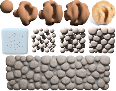
Rather than using the tangent-point energy to edit or process existing data, we can also use it to generate new geometry. In nature, the growth of organic shapes is often governed by simple combinations of objectives, e.g., a balance between area and volume while avoiding self-collision. We can likewise use such forces to drive the growth of organic-looking objects, such as the “walnut” depicted in Figure 22, top. The same technique is used in Figure 22, bottom, where multiple objects are packed into a volume to create a repeating organic pattern.

9.2.4. Collision Resolution

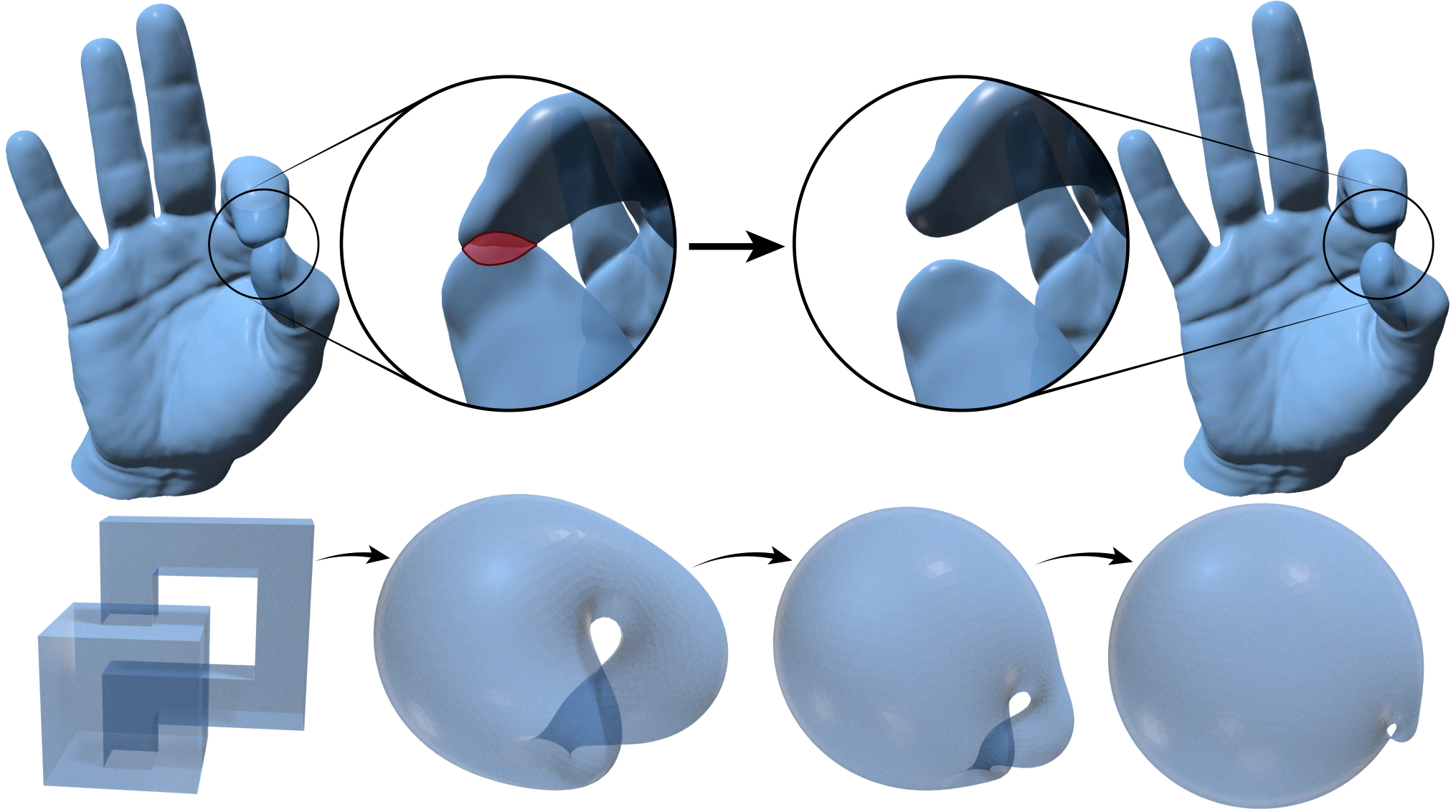
In many geometry processing tasks, input data is not free of self-intersections. For exponents $p>4$ , the tangent-point energy $\mathcal{E}^{p}$ of a non-embedded surface is infinite; to resolve intersections in the input, we can try reducing the exponent to a value $p<4$ , at which point $\mathcal{E}^{p}$ becomes finite but still discourages collision. Here we find that it also helps to disable the low-order term from Equation 8. Empirically, the same system framework now appears capable of eliminating small self-intersections (Figure 23, top), through struggles in more difficult scenarios like the Klein bottle depicted in Figure 23, bottom, which cannot be globally embedded without self-intersection. Further analysis of the energy for these “subcritical” values may help to provide more robust tools for global collision resolution.

10. Limitations and Future Work

The experiments from Section 9 suggest many opportunities for improvement. For instance, significant performance gains could be achieved purely through better software engineering, e.g., improving our parallel implementation of hierarchical matrix multiplication (which is currently bottlenecked around 4–8 threads), or implementing curvature-adaptive remeshing (à la [Dunyach et al. 2013]), rather than finely tessellating the whole domain. It would also be quite useful to track mesh attributes across remeshing operations, to enable (for instance) mapping of data from one shape to another through the canonical minimizer. Since we discretize tangent-point energy, we can provide no formal guarantee that collisions will not occur—as in Yu et al. 2021, a pragmatic solution would be to use continuous-time collision detection to limit the time step (or simply provide a certificate).

Several issues require deeper investigation. For one thing, unlike Yu et al. 2021, our preconditioning strategy cannot easily accommodate dense constraints (e.g., preservation of each triangle area), which would require a prohibitive number of iterative solves. Here one can instead use a stiff penalty; revisiting the multigrid approach via hierarchical coarsening [Botsch and Kobbelt 2004; Shi et al. 2006] may also prove fruitful. Our approximation of tangent-point energy becomes inaccurate in situations of very tight contact (à la Sections 9.2.1 and 9.2.2), since we effectively have few quadrature points per unit surface area; adding additional quadrature points (or adaptive refinement) to elements in near-contact may help to achieve tighter fits. For shape interpolation and mathematical visualization, it would be quite useful to find the trajectory that minimizes overall tangent-point energy, rather than just flowing to a common minimizer—here ideas about shell-space geodesics may prove valuable [Heeren et al. 2012]. Likewise, integrating repulsive regularization into a thin shell model might provide better proximity-aware shape editing by retaining a “memory” of the initial shape. Finally, we do not directly treat boundary conditions, or more general arrangements of repulsive curves and surfaces that might have interesting modeling applications.

Acknowledgments

The authors thank Saul Schleimer and Henry Segerman for helpful discussions about topological examples. This work was supported by a Packard Fellowship, NSF Award 1717320, and gifts from Autodesk, Activision Blizzard, Adobe, Disney, and Facebook. The third author was supported by DFG-Project 282535003: Geometric curvature functionals: energy landscape and discrete methods.

References

[1]
Barnes and Hut [1986] J. Barnes and P. Hut. 1986. A hierarchical O(N log N) force-calculation algorithm. Nature 324, 6096 (1986), 446–449.
Bednorz and Bednorz [2019] Adam Bednorz and Witold Bednorz. 2019. Analytic sphere eversion using ruled surfaces. Differential Geometry and its Applications 64 (2019), 59–79.
Blatt [2013] S. Blatt. 2013. The Energy Spaces of the Tangent Point Energies. Journal of Topology and Analysis 5, 3 (2013), 261–270.
Blatt and Reiter [2015] Simon Blatt and Philipp Reiter. 2015. Regularity theory for tangent-point energies: the non-degenerate sub-critical case. Adv. Calc. Var. 8, 2 (2015), 93–116. https://doi.org/10.1515/acv-2013-0020
Bobenko and Schröder [2005] Alexander I. Bobenko and Peter Schröder. 2005. Discrete Willmore Flow. In Proceedings of the Third Eurographics Symposium on Geometry Processing (Vienna, Austria) (SGP ’05). Eurographics Association, Goslar, DEU, 101–es.
Botsch and Kobbelt [2004] Mario Botsch and Leif Kobbelt. 2004. A Remeshing Approach to Multiresolution Modeling. In Proceedings of the 2004 Eurographics/ACM SIGGRAPH Symposium on Geometry Processing (Nice, France) (SGP ’04). Association for Computing Machinery, New York, NY, USA, 185–192.
Bridson et al. [2002] Robert Bridson, Ronald Fedkiw, and John Anderson. 2002. Robust treatment of collisions, contact and friction for cloth animation. In Proceedings of the 29th annual conference on Computer graphics and interactive techniques. 594–603.
Buck and Orloff [1995] G. Buck and J. Orloff. 1995. A simple energy function for knots. Top. Appl. 61, 3 (1995).
Bucur and Butazzo [2006] Dorin Bucur and Giuseppe Butazzo. 2006. VARIATIONAL METHODS IN SHAPE OPTIMIZATION PROBLEMS.
Chen and Holst [2011] Long Chen and Michael Holst. 2011. Efficient mesh optimization schemes based on Optimal Delaunay Triangulations. Computer Methods in Applied Mechanics and Engineering 200, 9 (2011), 967 – 984.
Chern et al. [2018] Albert Chern, Felix Knöppel, Ulrich Pinkall, and Peter Schröder. 2018. Shape from metric. ACM Transactions on Graphics (TOG) 37, 4 (2018), 1–17.
Claici et al. [2017] Sebastian Claici, Mikhail Bessmeltsev, Scott Schaefer, and Justin Solomon. 2017. Isometry-aware preconditioning for mesh parameterization. In Computer Graphics Forum, Vol. 36. Wiley Online Library, 37–47.
Clarenz et al. [2004] Ulrich Clarenz, Udo Diewald, Gerhard Dziuk, Martin Rumpf, and R Rusu. 2004. A finite element method for surface restoration with smooth boundary conditions. Computer Aided Geometric Design 21, 5 (2004), 427–445.
Crane et al. [2013] Keenan Crane, Ulrich Pinkall, and Peter Schröder. 2013. Robust Fairing via Conformal Curvature Flow. ACM Trans. Graph. 32, 4 (2013).
Desbrun et al. [1999] Mathieu Desbrun, Mark Meyer, Peter Schröder, and Alan H Barr. 1999. Implicit fairing of irregular meshes using diffusion and curvature flow. In Proceedings of the 26th annual conference on Computer graphics and interactive techniques. 317–324.
Droske and Rumpf [2004] Marc Droske and Martin Rumpf. 2004. A level set formulation for Willmore flow. Interfaces and free boundaries 6, 3 (2004), 361–378.
Dunyach et al. [2013] Marion Dunyach, David Vanderhaeghe, Loïc Barthe, and Mario Botsch. 2013. Adaptive remeshing for real-time mesh deformation. In Eurographics 2013. The Eurographics Association.
Dziuk [2008] Gerhard Dziuk. 2008. Computational parametric Willmore flow. Numer. Math. 111, 1 (2008), 55–80. https://doi.org/10.1007/s00211-008-0179-1
Eckstein et al. [2007] Ilya Eckstein, Jean-Philippe Pons, Yiying Tong, C.-C. Jay Kuo, and Mathieu Desbrun. 2007. Generalized Surface Flows for Mesh Processing. In Proceedings of the Fifth Eurographics Symposium on Geometry Processing (Barcelona, Spain) (SGP ’07). Eurographics Association, 183–192. https://doi.org/10.2312/SGP/SGP07/183-192
Elsey and Esedoḡlu [2009] Matthew Elsey and Selim Esedoḡlu. 2009. Analogue of the total variation denoising model in the context of geometry processing. Multiscale Modeling & Simulation 7, 4 (2009), 1549–1573.
Francis et al. [1997] George Francis, John M Sullivan, Rob B Kusner, Ken A Brakke, Chris Hartman, and Glenn Chappell. 1997. The minimax sphere eversion. In Visualization and mathematics. Springer, 3–20.
Francis and Francis [1987] George K Francis and GK Francis. 1987. A topological picturebook. Vol. 2. Springer.
Gillespie et al. [2021] Mark Gillespie, Boris Springborn, and Keenan Crane. 2021. Discrete Conformal Equivalence of Polyhedral Surfaces. ACM Trans. Graph. 40, 4 (2021).
Grinspun et al. [2003] Eitan Grinspun, Anil N Hirani, Mathieu Desbrun, and Peter Schröder. 2003. Discrete shells. In Proceedings of the 2003 ACM SIGGRAPH/Eurographics symposium on Computer animation. Citeseer, 62–67.
Hackbusch [2015] W. Hackbusch. 2015. Hierarchical matrices: algorithms and analysis. Vol. 49. Springer.
Hanocka et al. [2020] Rana Hanocka, Gal Metzer, Raja Giryes, and Daniel Cohen-Or. 2020. Point2Mesh: A Self-Prior for Deformable Meshes. ACM Trans. Graph. 39, 4, Article 126 (July 2020), 12 pages.
Harmon et al. [2011] David Harmon, Daniele Panozzo, Olga Sorkine, and Denis Zorin. 2011. Interference-aware geometric modeling. ACM Transactions on Graphics (TOG) 30, 6 (2011), 1–10.
Heeren et al. [2012] Behrend Heeren, Martin Rumpf, Max Wardetzky, and Benedikt Wirth. 2012. Time-discrete geodesics in the space of shells. In Computer Graphics Forum, Vol. 31. Wiley Online Library, 1755–1764.
Ishii [2008] Atsushi Ishii. 2008. Moves and invariants for knotted handlebodies. Algebraic & Geometric Topology 8, 3 (2008), 1403–1418.
Ishii et al. [2012] Atsushi Ishii, Kengo Kishimoto, Hiromasa Moriuchi, and Masaaki Suzuki. 2012. A table of genus two handlebody-knots up to six crossings. Journal of Knot Theory and Its Ramifications 21, 04 (2012), 1250035.
Joshi and Séquin [2007] Pushkar Joshi and Carlo Séquin. 2007. Energy minimizers for curvature-based surface functionals. Computer-Aided Design and Applications 4, 5 (2007), 607–617.
Kazhdan et al. [2012] Michael Kazhdan, Jake Solomon, and Mirela Ben-Chen. 2012. Can mean-curvature flow be modified to be non-singular?. In Computer Graphics Forum, Vol. 31. Wiley Online Library, 1745–1754.
Kobbelt et al. [1999] Leif P. Kobbelt, Jens Vorsatz, and Ulf Labsik. 1999. A Shrink Wrapping Approach to Remeshing Polygonal Surfaces. Computer Graphics Forum 18, 3 (1999), 119–130.
Kolasiński et al. [2015] Sławomir Kolasiński, Paweł Strzelecki, and Heiko von der Mosel. 2015. Compactness and isotopy finiteness for submanifolds with uniformly bounded geometric curvature energies. arXiv:arXiv:1504.04538
Kovalsky et al. [2016] Shahar Z. Kovalsky, Meirav Galun, and Yaron Lipman. 2016. Accelerated Quadratic Proxy for Geometric Optimization. ACM Trans. Graph. 35, 4, Article 134 (July 2016), 11 pages.
Kusner and Sullivan [1998] Robert B Kusner and John M Sullivan. 1998. Möbius-invariant knot energies. Ideal knots 19 (1998), 315–352.
Kwaśnicki [2017] Mateusz Kwaśnicki. 2017. Ten equivalent definitions of the fractional laplace operator. Fractional Calculus and Applied Analysis 20, 1 (Jan 2017).
Lackenby [2016] Marc Lackenby. 2016. Elementary knot theory. arXiv preprint arXiv:1604.03778 (2016).
Levy and Thurston [1995] Silvio Levy and William P Thurston. 1995. Making waves: A guide to the ideas behind Outside In. Geometry Center.
Marques and Neves [2014] Fernando C Marques and André Neves. 2014. Min-max theory and the Willmore conjecture. Annals of mathematics (2014), 683–782.
Martin et al. [2013] Tobias Martin, Pushkar Joshi, Miklós Bergou, and Nathan Carr. 2013. Efficient Non-linear Optimization via Multi-scale Gradient Filtering. In Computer Graphics Forum, Vol. 32. Wiley Online Library, 89–100.
Moreton and Séquin [1992] Henry P Moreton and Carlo H Séquin. 1992. Functional optimization for fair surface design. ACM SIGGRAPH Computer Graphics 26, 2 (1992), 167–176.
O’Hara [1991] Jun O’Hara. 1991. Energy of a knot. Topology 30, 2 (1991), 241–247.
Osher and Fedkiw [2006] Stanley Osher and Ronald Fedkiw. 2006. Level set methods and dynamic implicit surfaces. Vol. 153. Springer Science & Business Media.
Pinkall and Polthier [1993] U. Pinkall and K. Polthier. 1993. Computing discrete minimal surfaces and their conjugates. Experimental mathematics 2, 1 (1993), 15–36.
Renka and Neuberger [1995] Robert J Renka and JW Neuberger. 1995. Minimal surfaces and Sobolev gradients. SIAM Journal on Scientific Computing 16, 6 (1995), 1412–1427.
Sacht et al. [2015] Leonardo Sacht, Etienne Vouga, and Alec Jacobson. 2015. Nested cages. ACM Transactions on Graphics (TOG) 34, 6 (2015), 1–14.
Scharein [1998] Robert Glenn Scharein. 1998. Interactive topological drawing. Ph.D. Dissertation. University of British Columbia.
Schmidt et al. [2020] Patrick Schmidt, Marcel Campen, Janis Born, and Leif Kobbelt. 2020. Inter-surface maps via constant-curvature metrics. ACM Transactions on Graphics (TOG) 39, 4 (2020), 119–1.
Schumacher [2017] Henrik Schumacher. 2017. On $H^{2}$ -gradient Flows for the Willmore Energy. arXiv preprint arXiv:1703.06469 (2017).
Shi et al. [2006] Lin Shi, Yizhou Yu, Nathan Bell, and Wei-Wen Feng. 2006. A Fast Multigrid Algorithm for Mesh Deformation. ACM Trans. Graph. 25, 3 (2006), 1108–1117.
Soliman et al. [2021] Yousuf Soliman, Albert Chern, Olga Diamanti, Felix Knöppel, Ulrich Pinkall, and Peter Schröder. 2021. Constrained Willmore Surfaces. ACM Trans. Graph. 40, 4 (2021).
Sorkine and Alexa [2007] Olga Sorkine and Marc Alexa. 2007. As-rigid-as-possible surface modeling. In Symposium on Geometry processing, Vol. 4. 109–116.
Strzelecki and von der Mosel [2013] PawełStrzelecki and Heiko von der Mosel. 2013. Tangent-point repulsive potentials for a class of non-smooth $m$ -dimensional sets in $\mathbb{R}^{n}$ . Part I: Smoothing and self-avoidance effects. J. Geom. Anal. 23, 3 (2013), 1085–1139. https://doi.org/10.1007/s12220-011-9275-z
Strzelecki and von der Mosel [2018] Paweł Strzelecki and Heiko von der Mosel. 2018. Geometric curvature energies: facts, trends, and open problems. In New directions in geometric and applied knot theory. De Gruyter, Berlin, 8–35.
Wells [1997] David Wells. 1997. The Penguin dictionary of curious and interesting numbers. Penguin.
Wriggers and Zavarise [2004] Peter Wriggers and Giorgio Zavarise. 2004. Computational contact mechanics. Encyclopedia of computational mechanics (2004).
Ye et al. [2018] Zi Ye, Olga Diamanti, Chengcheng Tang, Leonidas Guibas, and Tim Hoffmann. 2018. A unified discrete framework for intrinsic and extrinsic Dirac operators for geometry processing. In Computer Graphics Forum, Vol. 37. Wiley Online Library, 93–106.
Yu et al. [2021] Chris Yu, Henrik Schumacher, and Keenan Crane. 2021. Repulsive Curves. ACM Trans. Graph. 40, 2, Article 10 (May 2021), 21 pages. https://doi.org/10.1145/3439429
Zhang [2005] Fuzhen Zhang. 2005. The Schur Complement and its Applications. Numerical Methods and Algorithms, Vol. 4. Springer, New York.
Zhu et al. [2018] Yufeng Zhu, Robert Bridson, and Danny M. Kaufman. 2018. Blended Cured Quasi-Newton for Distortion Optimization. ACM Trans. Graph. 37, 4, Article 40 (2018), 14 pages.

Appendix A Action of the Fractional Operators

In section Section 5.1 we claimed that the actions of the fractional operators $L^{\sigma}$ , $B$ , and $B_{0}$ can be expressed by suitable kernel matrices that we then compress by hierarchical methods. This is not obvious, so we include a brief derivation here. Consider the kernel matrix

H_{ST}:=(1-\delta_{ST})\,\lvert{X_{f}(S)-X_{f}(T)}\rvert^{-(2\sigma+2)}.

Rewriting Equation 11 for general $\mathbf{u}$ and $\mathbf{v}\in\mathbb{R}^{\lvert{V}\rvert}$ in terms of this kernel yields

\textstyle\mathbf{u}^{\mathsf{T}}L^{\sigma}\mathbf{v}=\sum_{S\in F}\sum_{T\in F}(\bar{u}(S)-\bar{u}(T))\,(\bar{v}(S)-\bar{v}(T))\,a_{f}(S)\,H_{ST}\,a_{f}(T).

Multiplying the product inside the sum gives

\big(\bar{u}(S)\,\bar{v}(S)+\bar{u}(T)\,\bar{v}(T)-\bar{u}(T)\,\bar{v}(S)-\bar{u}(S)\,\bar{v}(T)\big)\,a_{f}(S)\,H_{ST}\,a_{f}(T)

for the pair $(S,T)$ . Because $H_{ST}=H_{TS}$ , we can move some terms between the summands for $(S,T)$ and $(T,S)$ , and thus reorganize the sum into

	$\displaystyle\mathbf{u}^{\mathsf{T}}L^{\sigma}\mathbf{v}$	$\displaystyle=\textstyle 2\,\sum_{S\in F}\sum_{T\in F}\big(\bar{u}(S)\,\bar{v}(S)-\bar{u}(S)\,\bar{v}(T)\big)\,a_{f}(S)\,H_{ST}\,a_{f}(T)$
		$\displaystyle=\textstyle 2\,\sum_{S\in F}\bar{u}(S)a_{f}(S)\left(a_{f}(S)^{-1}\sum_{T\in F}H_{ST}a_{f}(T)\right)a_{f}(S)\bar{v}(S)$
		$\displaystyle\qquad-\textstyle 2\,\sum_{S\in F}\sum_{T\in F}\bar{u}(S)\,a_{f}(S)\,H_{ST}\,a_{f}(T)\,\bar{v}(T).$

Recall that $\mathsf{U}\in\operatorname{Hom}(\mathbb{R}^{\lvert{V}\rvert};\mathbb{R}^{\lvert{F}\rvert})$ is defined by $(\mathsf{U}\mathbf{u})(S)=a_{f}(S)\bar{u}(S)$ . Thus the above collapses to

	$\displaystyle\mathbf{u}^{\mathsf{T}}L^{\sigma}\mathbf{v}$	$\displaystyle=2\,\mathbf{u}^{\mathsf{T}}\mathsf{U}^{\mathsf{T}}\diag(a_{f})^{-1}\diag(H\,a_{f})\,\mathsf{U}\,\mathbf{v}-2\,\mathbf{u}^{\mathsf{T}}\mathsf{U}^{\mathsf{T}}H\,\mathsf{U}\,\mathbf{v}$
		$\displaystyle=2\,\mathbf{u}^{\mathsf{T}}\mathsf{U}^{\mathsf{T}}\big[\diag\big(\diag(a_{f})^{-1}H\,a_{f}\big)-H\big]\,\mathsf{U}\,\mathbf{v}.$

The derivation follows analogously for the high- and low-order matrices $B$ and $B_{0}$ , with the substitution of the operator $\mathsf{V}=\diag(a_{f})\mathsf{D}_{f}$ for $\mathsf{U}$ in the case of $B$ .

Appendix B Fast Matrix-Vector Multiplication

Step 1 of Section 5.1.5 corresponds to thinning out the matrix shown in Figure 6 by removing all the green parts. The remainder is a sparse block matrix with variable block size. We store this sparse matrix in CSR format and perform matrix-vector multiplication via sparse BLAS routines.

In Step 2 the kernel matrix $H_{{\mathcal{I}}{\mathcal{J}}}$ is compressed into the rank-one-matrix $\mathbf{1}_{\mathcal{I}}\,h(X_{{\mathcal{I}}},P_{{\mathcal{I}}};X_{{\mathcal{J}}},P_{{\mathcal{J}}})\,\mathbf{1}_{\mathcal{J}}^{\mathsf{T}}$ . In this step, we are cautious not to move the input data $\mathbf{x}_{\mathcal{J}}$ and output data $\mathbf{y}_{\mathcal{I}}$ directly to and from the clusters ${\mathcal{I}}$ and ${\mathcal{J}}$ . Instead, we employ a common technique for fast multipole and hierarchical matrix methods and use the BVH for that. For each cluster ${\mathcal{I}}$ , ${\mathcal{J}}$ , we allocate scalars $\tilde{x}_{{\mathcal{J}}}$ and $\tilde{y}_{{\mathcal{I}}}$ . We start only with the leaf clusters and set

\tilde{x}_{{\mathcal{J}}}\leftarrow\textstyle\sum_{T\in{\mathcal{J}}}\mathbf{x}(T)\quad\text{for each leaf cluster ${\mathcal{J}}$.}

Then, during a parallel traversal of the BVH in post-order, for each cluster ${\mathcal{J}}$ , we add the $\tilde{x}$ -values of its children into $\tilde{x}_{{\mathcal{J}}}$ . After this upward pass is finished, we loop over all clusters ${\mathcal{I}}$ and set

(20)

\displaystyle\tilde{y}_{{\mathcal{I}}}\leftarrow\textstyle\sum_{{\mathcal{J}}}h(X_{{\mathcal{I}}},P_{{\mathcal{I}}};X_{{\mathcal{J}}},P_{{\mathcal{J}}})\,\tilde{x}_{{\mathcal{J}}},

where the sum runs over the ${\mathcal{J}}$ such that $({\mathcal{I}},{\mathcal{J}})$ is admissible. This operation is also best performed by a sparse matrix multiplication. To this end, we fix an ordering of the BVH clusters, e.g., depth-first ordering. Then we assemble a sparse matrix $\tilde{H}$ with the nonzero value $h(X_{{\mathcal{I}}},P_{{\mathcal{I}}};X_{{\mathcal{J}}},P_{\mathcal{J}})$ at the position that correspond to the admissible block cluster $({\mathcal{I}},{\mathcal{J}})$ . Storing $\tilde{x}$ and $\tilde{y}$ as vectors, Equation 20 amounts to

\displaystyle\tilde{y}\leftarrow\tilde{H}\,\tilde{x}.

Afterwards, we use a downward pass through the BVH to distribute the $\tilde{y}$ -values back into the vector $\mathbf{y}$ : We traverse the BVH in pre-order and let each cluster ${\mathcal{I}}$ add its $\tilde{y}$ -value into each of its children’s $\tilde{y}$ -values. Finally each leaf cluster adds its value into each of its member’s $\mathbf{y}$ -entry, i.e.,

\displaystyle\mathbf{y}(S)\leftarrow\mathbf{y}(S)+\tilde{y}_{{\mathcal{I}}}\quad\text{for each leaf ${\mathcal{I}}$ and each $S\in{\mathcal{I}}$.}

The structure of the kernel matrices of $L^{\sigma}$ , $B$ , and $B_{0}$ is very similar. This allows us to use a single block cluster tree to compress all of them. Moreover, the sparsity patterns for the two sparse matrices used to perform Steps 1 and 2 can be shared and the corresponding nonzero values can be computed in a single parallelized loop over the admissible and inadmissible blocks, respectively.

For the application of $A_{3}$ to a vector $\mathbf{v}$ of size $3\lvert{V}\rvert$ , we could apply $A=B+B_{0}$ separately on three vectors $\mathbf{v}_{1}$ , $\mathbf{v}_{2}$ , and $\mathbf{v}_{3}$ of size $\lvert{V}\rvert$ that each store only one spatial component of the vertex positions. However, it turns out to be more efficient to store $\mathbf{v}_{1}$ , $\mathbf{v}_{2}$ , and $\mathbf{v}_{3}$ as columns of a matrix of size $\lvert{V}\rvert\times 3$ and to replace the sparse matrix-vector products by sparse matrix-dense matrix products.