Decentralized Trajectory Optimization
for Multi-Agent Ergodic Exploration Thanks: Manuscript received: February, 24, 2021; Revised May, 26, 2021; Accepted June, 22, 2021.Thanks: This paper was recommended for publication by Editor Lucia Pallottino upon evaluation of the Associate Editor and Reviewers’ comments. This work has been partially supported by the Swiss National Science Foundation under NCCR Automation. Thanks:  The authors are with the Department of Information Technology and Electrical Engineering, Automatic Control Lab, ETH, Zürich 8092, Switzerland. (corresponding author: Andrea Iannelli) emails: dgkouletsos@student.ethz.ch, {iannelli, mbadyn, lygeros} @control.ee.ethz.ch Thanks: Digital Object Identifier (DOI): see top of this page.

All agents maintain estimates of the trajectories of all other agents, thus denote by $\left\{\eta^{(\ell)}\right\}_{j}$ the feasible trajectory of the $\ell$-th agent estimated by the $j$-th agent, and by $\left\{\eta\right\}_{j}=\left(\left\{\eta^{(1)}\right\}_{j},\ldots,\left\{\eta^{(N)}\right\}_{j}\right)$ the stacked vector. Same convention is used for the planning trajectories $\xi$.

At iteration $i$, each agent determines its descent direction $\zeta_{i}^{(j)}$ to minimize locally the objective function $J$. To this end, the objective function $J$ is approximated by a second-order Taylor expansion around $\xi_{i}^{(j)}$

where $T_{\xi^{(j)}_{i}}\mathcal{T}$ is the tangent trajectory manifold of $\mathcal{T}$, $D_{\xi_{i}^{(j)}}J\left(\left\{\xi_{i}\right\}_{j}\right)\circ\zeta_{i}^{(j)}$ is the first Frechet directional derivative and $\left(\zeta_{i}^{(j)},\zeta_{i}^{(j)}\right)$ is a quadratic approximation of the second Frechet directional derivative. The constraints force the direction $\zeta^{(j)}_{i}$ to lie on the tangent space of the trajectory manifold $\mathcal{T}$ [14]. The direction $\zeta_{i}^{(j)}=\left(z_{i}^{(j)},v_{i}^{(j)}\right)$ is divided into state direction $z_{i}^{(j)}$ and control direction $v_{i}^{(j)}$. For clarity, we omit the iteration subscript $i$ and assume that a feasible trajectory $\eta^{(j)}$ is available (this is natural considering that projection operator $\mathcal{P}$ is applied at the end of each iteration).

To update the current planning trajectory $\xi^{(j)}_{i}$ with respect to the descent direction $\zeta^{(j)}_{i}$, we adopt the common Armijo rule [18]. The optimal step-size is defined as

where the user-defined parameter $\rho$ sets the desired magnitude decrease required to achieve an adequate objective improvement. It is important to observe that the Armijo rule needs global information to guarantee the cost function decrease. Here, in line with the approximation proposed for step one, each agent implements a local version of the rule using the current iterates of the neighbours and the estimates of the trajectories of all other agents. This is a heuristic, whose suboptimality we intend to analyse in future research. A starting point could be extending the local Armijo rule for strictly convex and separable cost functions with linear constraints developed in [19] to the non-convex setting analyzed in this paper.

The projection operator $\mathcal{P}$ maps a planning trajectory into the closest one belonging to the trajectory manifold $\mathcal{T}$ made of trajectories that satisfy $\dot{x}^{(j)}=f(x^{(j)},u^{(j)})$, that is $\mathcal{P}:\xi^{(j)}=(\alpha^{(j)},\mu^{(j)})\mapsto\eta^{(j)}=(x^{(j)},u^{(j)})$. It was shown in [14] that the projection operator $\mathcal{P}$ can be interpreted as the following trajectory tracking controller

The optimal controller gain $K^{(j)}$ can be computed as the solution of a finite horizon Linear Quadratic Regulator problem [17] applied to a linearization of the nonlinear dynamics around the trajectory $\xi^{(j)}=(\alpha^{(j)},\mu^{(j)})$. A useful criterion for choosing the weighting matrices $R_{LQR}\in\mathbb{R}^{m\times m}$ and $Q_{LQR}\in\mathbb{R}^{n\times n}$ is to tune them so that the projected trajectory $\eta^{(j)}$ is close to $\xi^{(j)}$ and thus the linearization gives sufficiently accurate results.

Agent $j$ has only access to the trajectories optimized by the agents in its neighbourhood $\mathcal{N}(j)$. At the end of round $i$, the vector of feasible trajectories estimated by the $j$-th agent $\left\{\eta^{(\ell)}\right\}_{j}$ is obtained by the communication protocol below

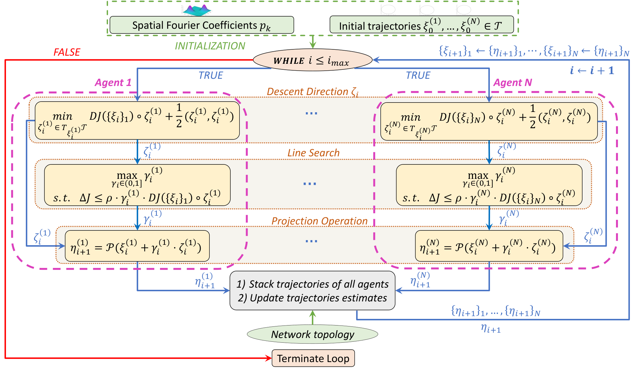
If an agent $\ell$ is not included in the neighbourhood of the $j$-th agent, then the $j$-th agent averages its estimate of agent $\ell$’s trajectories with its neighbours’ estimates of agent $\ell$’s trajectory. Figure 2 illustrates a flowchart of the iterative optimization algorithm.

The termination criterion consists of stopping the algorithm after a maximum number of iterations $i_{max}$ has been performed. Because the algorithm is run offline, the value of $i_{max}$ can be chosen large enough so that the ergodic reduction metric $\mathcal{E}_{r}:=100\frac{\mathcal{E}_{0}-\mathcal{E}_{f}}{\mathcal{E}_{0}}$, where $\mathcal{E}_{f}$ and $\mathcal{E}_{0}$ are the ergodicity at the $i_{max}$-th and initial trajectory, respectively, has a satisfactory value. Alternatively, each agent can broadcast to its neighbours a flag when its local problem has reached the termination criterion (which can include e.g. a local estimate of $\mathcal{E}_{r}$ and the local directional derivative), which in subsequent iterations is rebroadcast to their (the neighbours’) neighbours, and so on. Once an agent has collected termination flags from all other agents, it ceases running the algorithm. This happens $G$ iterations after all agents have reached their respective local termination criteria, where $G$ is the length of the longest path in the graph (or girth).

We consider the nonlinear dynamic model for the motion of the single agent used in [4] and a time horizon $T=3.5\text{ sec}$. That is

The state vector is $x^{(j)}=\left[X^{(j)},Y^{(j)},\theta^{(j)}\right]^{\top}$ where $X^{(j)}$ and $Y^{(j)}$ correspond to Cartesian coordinates, while $\theta^{(j)}$ is the heading angle of the velocity vector. The control input vector $u^{(j)}=\left[\nu^{(j)},\omega^{(j)}\right]^{\top}$ consists of the forward velocity $\nu^{(j)}$ and the time derivative $\omega^{(j)}$ of the heading angle $\theta^{(j)}$. The initial feasible trajectories are circles with radius $\mathcal{R}=0.05\text{ m}$ and center randomized as discussed later.

The exploration field is assumed to be a two-dimensional space $\left[0,1\right]\times\left[0,1\right]$ corresponding to $X$ and $Y$ Cartesian coordinates and, thus, the number of exploratory variables is $\lambda=2$ . The information density, assigned to this field, is modelled based on a Gaussian mixture structure as follows

where: $M=\begin{bmatrix}1&0&0\\ 0&1&0\end{bmatrix}$ is a transformation that maps $\chi$ to the exploration variables; $\mu_{i}\in\mathbb{R}^{2}$ is the mean vector of the $i$-th mode; $\Sigma_{i}\in\mathbb{R}^{2\times 2}$ is the positive definite covariance of the $i$-th mode; and $w_{i}\in[0,1]$ is the weight of the $i$-th mode (chosen such that $p$ integrates to 1 in the exploration domain). To investigate the ability of the algorithm to design different planning strategies as a function of the information densities, we investigate two different cases for (17). The first, named volcano, has a dominant mode at the center of the exploration map and other minor modes peripherally. The first mode has $w_{1}=0.6$, $\Sigma_{1}=0.014\cdot\mathcal{I}_{2\times 2}$ and $\mu_{1}=\begin{bmatrix}0.5&0.5\end{bmatrix}^{\top}$, whereas the rest of the modes are equally weighted with $\Sigma_{i}=0.004\cdot\mathcal{I}_{2\times 2}$, $\mu_{2}=\begin{bmatrix}0.75&0.5\end{bmatrix}^{\top}$, $\mu_{3}=\begin{bmatrix}0.25&0.5\end{bmatrix}^{\top}$ $\mu_{4}=\begin{bmatrix}0.5&0.75\end{bmatrix}^{\top}$ and $\mu_{5}=\begin{bmatrix}0.5&0.25\end{bmatrix}^{\top}$. The second, named archipelago, has four modes with same covariance $\Sigma=0.006\cdot\mathcal{I}_{2\times 2}$ and mean vectors $\mu_{1}=\begin{bmatrix}0.25&0.25\end{bmatrix}^{\top}$, $\mu_{2}=\begin{bmatrix}0.75&0.25\end{bmatrix}^{\top}$, $\mu_{3}=\begin{bmatrix}0.25&0.75\end{bmatrix}^{\top}$, $\mu_{4}=\begin{bmatrix}0.75&0.75\end{bmatrix}^{\top}$.

The approximation of spatial and trajectory distributions is addressed through the basis functions (2), where we set $K_{1}=K_{2}=10$ for $X$ and $Y$ coordinates, respectively, and $K_{3}=0$ for $\theta$ coordinate as there is no exploration. It is noted that an increase in state dimension (16) has no effect on the computation of the coefficients, since one would assign zero to the indexes $K_{j}$ associated with non-exploratory states $j$. Since the planning is done off-line, considering a higher order system would have little impact on the rest of the trajectory optimization problem.

Table I summarizes design parameters for the trajectory optimization algorithm. In the objective function, we prioritize ergodicity against control energy by adjusting accordingly the relative magnitudes of $q$ and $R$. It can also be observed that matrix $W_{jl}=W$ extracts from the state vector elements related to Cartesian coordinates so that a Euclidean distance metric is obtained in the inter-agent cost term. The choice for $Q_{n}$ and $R_{n}$ is motivated by a desired smooth change on the state $x$ and a more aggressive change on control $u$, respectively. The LQR weighting matrices have been tuned according to the previously discussed criterion.

For the line search problem (13), we parameterize $\gamma^{(j)}_{i}=\beta^{h}$ with $\beta=0.99$. With this choice, a fine search on the step-size is allowed and, thus, a larger reduction of the objective function is achieved, with convergence benefits [20]. Parameter $\rho$ specifies the magnitude of reduction in the sufficient decrease condition and a typical value $\rho=10^{-4}$ is used. Finally, the termination criterion is $i_{max}$ $=$ $70$.

The analyzed network topologies for 3$\leq N\leq$10 were randomly generated and are shown in Fig. 3. This topology defines the fixed neighbourhood $\mathcal{N}(\cdot)$ used in (15) and establishing the communication constraints among the agents.

The performance of the algorithm is investigated based on the four metrics defined below (the first two are global, while the last two are at agent-level):

• •

  Optimal temporal ergodic metric [3]:

  $$\mathcal{E}_{opt}(t)=\sum_{k\in\mathcal{K}}\Lambda_{k}\left(C_{k}\left(x^{*},t\right)-p_{k}\right)^{2},$$

  (18)

  where $C_{k}(x,t)=\frac{1}{N}\sum_{j=1}^{N}\frac{1}{t}\int_{0}^{t}F_{k}\left(x^{(j)}(\tau)\right)d\tau$. This is a time-dependent feature as it evaluates ergodicity with respect to any time instant in the horizon.

• •

  Completion task time [9, 10]: it is generally used to indicate the time $t_{CTT}$ at which exploration can terminate without loss of beneficial information. In this work, we define it as the first time instance $t\in[0,T]$ when $\frac{\mathcal{E}_{opt}(t=0)-\mathcal{E}_{opt}(t)}{\mathcal{E}_{opt}(t=0)}\geq\epsilon_{opt}$ , where $\epsilon_{opt}$ is defined in Section V.

• •

  Control energy per agent: $\sqrt{\int_{0}^{t_{CTT}}u^{(j)}(\tau)^{2}d\tau}.$

• •

  Traveled Distance: $\int_{0}^{t_{CTT}}\lvert\nu^{(j)}(\tau)\rvert d\tau.$

A comparison between the optimal trajectories in the Cartesian coordinates for single-agent ($a$) and 5-agent cases ($b$) with respect to the two information density distributions discussed earlier is presented in Figures 4 and 5. The figures also show the optimal ergodic metric $\mathcal{E}_{opt}$ ($t$) as a function of the time inside the horizon $t$. The inter-agent distance penalty term and optimal temporal ergodicity reduction tolerance are set to $r=1$ and $\epsilon_{opt}=99.5$, respectively. The initial trajectories used in the optimization are represented in dashed line, while the system’s state initial condition $x_{0}$ at $t=0$ is picked in low interest regions.

Figure 4(a) shows how the single-agent attempts to cover the whole region by spending more time in regions of higher interest, according to the ergodic principle. However, a high amount of time is required to cover efficiently the domain as shown by the completion task time value $t_{CTT}=3.06\text{ sec}$. On the other hand, in the multi-agent case in Fig. 4(b), the agents collaborate and split the field into exploration sub-domains. This is enabled by the use of a shared ergodic metric $\mathcal{E}$ in the objective function (5) that frames exploration as a common group task among the agents. As a result, a more time-efficient exploratory mission compared to the single-agent case is accomplished (note that $t_{CTT}=1.66\text{ sec}$ value in Fig. 4(b)). Figure 4(c), which displays the time-dependent optimal ergodic metric $\mathcal{E}_{opt}$, shows another distinctive feature of the multi-agent solution. Namely, $\mathcal{E}_{opt}$ is monotonic with respect to time in the 5-agent case, unlike in the single-agent case. This can be explained by observing that the single-agent in Fig. 4(a) displays an initially efficient area coverage around high-valued information regions, but afterwards it spends a fraction of time in a low-valued information. This is necessary to move towards different high-valued regions, and determines the temporary increase of $\mathcal{E}_{opt}$. On the contrary, in the multi-agent case this inefficient part can be avoided by leveraging the possibility to optimize over multiple trajectories and thus distribute exploration to maximize the information reward. This feature, which had not been previously observed to the best of the authors knowledge, points out an additional benefit of the multi-agent configuration. Indeed, if $\mathcal{E}_{opt}$ is monotonic, one is guaranteed to improve, in an ergodic sense, on learning the exploration field as time proceeds.

Figure 5 presents similar analyses for the Archipelago distribution. The single-agent visits all four modes spending more time in regions close to the peaks of the modes (Figure 5(a)), achieving a completion time ($t_{CTT}=3.17\text{ sec}$) which is again very close to the horizon $T$ of the mission. Collaborative planning is again observed for the 5-agent case in Fig. 5(b), where it is noted that the five initial trajectories are chosen very close to each other. Nonetheless, the optimized trajectories are distinct and allow the swarm to efficiently cover all modes ( $t_{CTT}=1.65\text{ sec}$). It is again instructive to observe the trend exhibited by the optimal ergodic metric $\mathcal{E}_{opt}$ (Fig. 5(c)). In a qualitatively similar manner as before, the single-agent trajectory initially a decrease in ergodicity due to the coverage of the mode on the top-right. However, when it is directed to the second it spends a great amount of time in the intermediate low-valued information region, determining an over-shoot in the plot. This is clearly avoided in the multi-agent scenario configuration.

We provide here a comprehensive analysis of the effect of increasing the number of agents and of choosing the initial conditions of the agents’ state on three performance metrics. The number of considered agents is varied from 1 to 10, and, in each case, the optimization algorithm is run using 100 random initializations for the agents initial location $x_{0}$. Precisely, we sample each initial condition from a uniform distribution such that $\theta(t=0)\in[0,2\pi]$, $X(t=0)\in[0.05,0.95]$ and $Y(t=0)\in[0.05,0.95]$. It is noted that this also randomizes the feasible trajectory used to initialize the optimization. As mentioned earlier, the trajectories are circles with given radius, and the selection of a point $x_{0}$, together with the constraint that the circular trajectory is feasible for the dynamics, uniquely determines its location in the field. These analyses thus shed also some light on the effect of the initial trajectory on the final result, which is an important aspect due to the non-convexity of the optimization problem.

Results are shown in terms of three performance metrics, namely the completion task time $t_{CTT}$, the control energy per agent, and the traveled distance $\mathcal{D}$. The inter-agent distance penalty term and optimal temporal ergodicity reduction tolerance are set to $r=3$ and $\epsilon_{opt}=98.5$, respectively.

Figures 6(a) and 6(b) show box plots of the completion task time statistics against number of agents for Volcano and Archipelago distributions, respectively. As expected, increasing the number of agents reduces the completion task time leading to more efficient exploration schemes. In the Volcano case, above 8 agents no further decrease is observed, suggesting that there is a distribution-dependent threshold for the largest number of agents giving an advantage in completion time. It is noted that $99.7\%$ and $92.4\%$ of the cases in Volcano and Archipelago distributions, respectively, have achieved an ergodicity reduction $\mathcal{E}_{r}$ above $95\%$.

Figure 7 presents the control energy performance for the most and least energy consuming agents.This analysis highlights the advantageous distribution of energy for a multi-agent system. Indeed, by increasing the agents number, each individual agent consumes lower energy and, thus, the energy pool is distributed efficiently among the agents.

Figure 8 finally shows the traveled distance box plot statistics. Recall that this metric is not explicitly targeted in the optimization, but it is nonetheless of practical interest to monitor it. As before, since this metric is a function of the agent, the minimum and maximum traveled distances are presented.Increasing the number of agents clearly leads to a decrease in the traveled distance. It is worth noting that it also leads to a decrease in the dispersion of this metric, both in terms of number of whiskers and box plots width.

Figure 9 reports the results of an investigation of the convergence properties of the decentralized algorithm. Specifically, the largest absolute value of the directional derivative across agents, i.e. $\underset{j\in\{1,\cdots,N\}}{\max}|D_{\xi_{i}^{(j)}}J\left(\xi_{i}\right)\circ\zeta_{i}^{(j)}|$, normalized by the initial trajectory directional derivative at $i=0$, is presented as a metric of optimality. The analyses are done on the graphs in Figure 3 for a randomly generated initial trajectory and initial condition $x_{0}$.

A sublinear rate can be recognized in both examples. It is also observed that, probably due to the heuristic decentralization of the Armijo line search, there is no monotonic decrease in the optimality metric. However, this does not compromise convergence. Analyses have also been carried out for two extreme network topologies, namely complete and line graphs, which showcased qualitatively similar trends (data not shown).

References

- [1] M. P. Christiansen, M. S. Laursen, R. N. Jørgensen, S. Skovsen, and R. Gislum, “Designing and testing a UAV mapping system for agricultural field surveying,” Sensors, vol. 17, no. 12: 2703, 2017.
- [2] J. Delmerico, E. Mueggler, J. Nitsch, and D. Scaramuzza, “Active autonomous aerial exploration for ground robot path planning,” IEEE Robotics and Automation Letters, vol. 2, no. 2, pp. 664–671, 2017.
- [3] G. Mathew and I. Mezić, “Metrics for ergodicity and design of ergodic dynamics for multi-agent systems,” Physica D: Nonlinear Phenomena, vol. 240, no. 4-5, pp. 432–442, 2011.
- [4] L. M. Miller and T. D. Murphey, “Trajectory optimization for continuous ergodic exploration,” in American Control Conference, 2013.
- [5] L. M. Miller, Y. Silverman, M. A. MacIver, and T. D. Murphey, “Ergodic exploration of distributed information,” IEEE Transactions on Robotics, vol. 32, no. 1, pp. 36–52, 2015.
- [6] E. Ayvali, H. Salman, and H. Choset, “Ergodic coverage in constrained environments using stochastic trajectory optimization,” in International Conference on Intelligent Robots and Systems (IROS), 2017.
- [7] H. Lee, H. Kim, and H. J. Kim, “Planning and control for collision-free cooperative aerial transportation,” IEEE Transactions on Automation Science and Engineering, vol. 15, no. 1, pp. 189–201, 2016.
- [8] J. G. Manathara, P. Sujit, and R. W. Beard, “Multiple UAV coalitions for a search and prosecute mission,” Journal of Intelligent & Robotic Systems, vol. 62, no. 1, pp. 125–158, 2011.
- [9] J. Hu, H. Niu, J. Carrasco, B. Lennox, and F. Arvin, “Voronoi-based multi-robot autonomous exploration in unknown environments via deep reinforcement learning,” IEEE Transactions on Vehicular Technology, vol. 69, no. 12, pp. 14 413 – 14 423, 2020.
- [10] T. Nestmeyer, P. R. Giordano, H. H. Bülthoff, and A. Franchi, “Decentralized simultaneous multi-target exploration using a connected network of multiple robots,” Autonomous Robots, vol. 41, p. 989–1011, 2017.
- [11] I. Abraham and T. D. Murphey, “Decentralized ergodic control: Distribution-driven sensing and exploration for multiagent systems,” IEEE Robotics and Automation Letters, vol. 3, no. 4, pp. 2987 – 2994, 2018.
- [12] H. Salman, E. Ayvali, and H. Choset, “Multi-agent ergodic coverage with obstacle avoidance,” in International Conference on Automated Planning and Scheduling, 2017.
- [13] A. Prabhakar, I. Abraham, A. Taylor, M. Schlafly, K. Popovic, G. Diniz, B. Teich, B. Simidchieva, S. Clark, and T. Murphey, “Ergodic specifications for flexible swarm control: From user commands to persistent adaptation,” Robotics: Science and Systems, 2020.
- [14] J. Hauser, “A projection operator approach to the optimization of trajectory functionals,” in 15th IFAC World Congress, 2002.
- [15] “Supplemental material to the paper ”Decentralized Trajectory Optimization for Multi-Agent Ergodic Exploration”,” DOI: 10.3929/ethz-b-000491536, 2021, ETH Research Collection.
- [16] A. Saccon, J. Hauser, and A. P. Aguiar, “Optimal Control on Lie Groups: The Projection Operator Approach,” IEEE Transactions on Automatic Control, vol. 58, no. 9, pp. 2230–2245, 2013.
- [17] B. D. Anderson and J. B. Moore, Optimal Control: Linear Quadratic Methods. Courier Corporation, 2007.
- [18] L. Armijo, “Minimization of functions having lipschitz continuous first partial derivatives,” Pacific Journal of mathematics, vol. 16, no. 1, pp. 1–3, 1966.
- [19] M. Zargham, A. Ribeiro, and A. Jadbabaie, “A distributed line search for network optimization,” in American Control Conference, 2012.
- [20] C. T. Kelley, Iterative Methods for Optimization. SIAM, 1999.