Certifiably Robust Interpretation via Rényi Differential PrivacyJournal: Artificial Intelligence

Ao Liu Email: liua6@rpi.edu Address: Department of Computer Science, Rensselaer Polytechnic Institute, Troy, NY, USA Xiaoyu Chen Address: Institute for Interdisciplinary Information Sciences, Tsinghua University, Beijing, China Sijia Liu Address: Department of Computer Science and Engineering, Michigan State University, 220 Trowbridge Rd, East Lansing, MI, USA Lirong Xia Address: Department of Computer Science, Rensselaer Polytechnic Institute, Troy, NY, USA Chuang Gan Address: MIT-IBM Watson AI Lab, 75 Binney St, Cambridge, MA, USA

Abstract

Motivated by the recent discovery that the interpretation maps of CNNs could easily be manipulated by adversarial attacks against network interpretability, we study the problem of interpretation robustness from a new perspective of Rényi differential privacy (RDP). The advantages of our Rényi-Robust-Smooth (RDP-based interpretation method) are three-folds. First, it can offer provable and certifiable top- $k$ robustness. That is, the top- $k$ important attributions of the interpretation map are provably robust under any input perturbation with bounded $\ell_{d}$ -norm (for any $d\geq 1$ , including $d=\infty$ ). Second, our proposed method offers $\sim$ 10% better experimental robustness than existing approaches in terms of the top- $k$ attributions. Remarkably, the accuracy of Rényi-Robust-Smooth also outperforms existing approaches. Third, our method can provide a smooth tradeoff between robustness and computational efficiency. Experimentally, its top- $k$ attributions are twice more robust than existing approaches when the computational resources are highly constrained.

Keywords:

Differential Privacy, Machine Learning, Robustness, Interpretation, and Neural Networks

1 Introduction

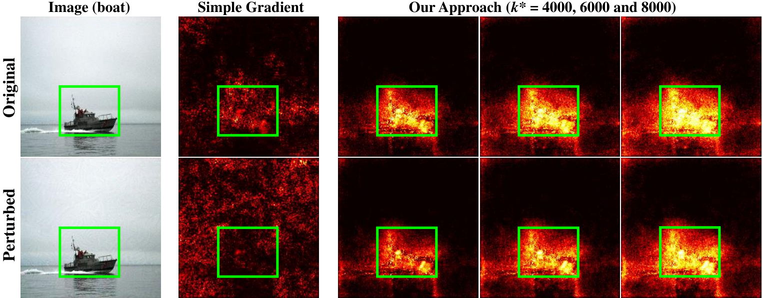
Convolutional neural networks (CNNs) have demonstrated successes on various computer vision applications, such as image classification [1, 2], object detection [3], semantic segmentation [4] and video recognition [5]. Spurred by the promising applications of CNNs, understanding why they make the correct prediction has become essential. The interpretation map explains which part of the input image plays a more important role in the prediction of CNNs. However, it has recently been shown that many interpretation maps, e.g., Simple Gradient [6], Integrated Gradient [7], DeepLIFT [8] and GradCam [9] are vulnerable to imperceptible input perturbations [10, 11]. In other words, slight perturbations to an input image could cause a significant discrepancy in its coupled interpretation map while keeping the predicted label unchanged (see an illustrative example in Figure 1).

Refer to caption — Figure 1: An example of the vulnerability of simple gradient. The green boxes annotate the position of the labeled object. Our approach offers stronger robustness against interpretation attacks. Remarkably, our interpretation also more accurately matches the position of the object.

Robustness of the interpretation maps is essential. Successful attacks can create confusions between the model interpreter and the classifier, which would further ruin the trustworthiness of systems that use the interpretations in down-stream actions, e.g., medical recommendation [12], source code captioning [13], and transfer learning [14]. In this paper, we aim to provide a framework to generate certifiably robust interpretation maps against $\ell_{d}$ -norm attacks, where $d\in[1,\infty]$ ¹¹ 1 In all discussions of this paper, we use $[1,\infty]$ to represent $[1,\infty)\cup\{\infty\}$ .. Our framework does not require the defender to know the type of attack, as long as it is an $\ell_{d}$ -norm attack. Our framework provides a stronger robustness guarantee if the exact attack type is known.

A Motivating Example. To better motivate and strengthen our claim, we present an experiment on real-world medical images: skin lesion diagnosis (see Figure 2, [15]). In this task, the ML classifier predicts a type of skin lesion, and an interpretation map can help doctors localize the most interpretable region responsible for the current prediction (e.g., the region highlighted by the red box in Figure 2). However, an adversary (that crafts imperceptible input perturbations) could fool interpretation map (for incorrect identification of region marked by the green box in Figure 2) under the same classification label. If doctors perform a medical diagnosis based on the fooled interpretation map, then the doctor will waste his/her time on treating the incorrect region. Figure 2 shows that our proposed robust interpretation can effectively defend such an adversary.

Differential privacy (DP) has recently been introduced as a tool to improve the robustness of machine learning algorithms. DP-based robust machine learning algorithms can provide theoretical robustness guarantees against adversarial attacks [16]. Rényi differential privacy (RDP) is a generalization of the standard notion of differential privacy. It has been proved that analyzing the robustness of CNNs using RDP can provide a stronger theoretical guarantee than standard DP [17]. However, the following question remains open.

How can we protect the interpretation map from $\ell_{d}$ attacks for $d\geq 3\;$ ?

This is the question we will address in this paper.

Our main theoretical contribution is the Rényi-Robust-Smooth framework (Algorithm 1) that provides a smooth tradeoff between interpretation robustness and computational-efficiency. Here, the robustness of interpretation is measured by the resistance to the top- $k$ attribution²² 2 Top- $k$ attribution refers to the top- $k$ important pixels (top- $k$ largest components) in the interpretation maps. change of an interpretation map when facing interpretation attacks. To prove the robustness of our framework, we firstly propose the new notion of Rényi robustness (Definition 3), which is directly connected with RDP and other robustness notions. Then, we show that the interpretation robustness can be guaranteed by Rényi robustness (Section 4). Our RDP-based analysis can provide significantly tighter robustness bound in comparison with the recently proposed interpretation method, Sparsified SmoothGrad [18] (Figure 5 left).

Experimentally, our Rényi-Robust-Smooth can provide $\sim$ 10% improvement on robustness in comparison with the state of the art (Figure 5 left). Surprisingly, our improvement of interpretation robustness does not come at the cost of accuracy. We found that the accuracy of Rényi-Robust-Smooth out-performs the recently-proposed approach of Sparsified SmoothGrad (Figure 5 right). Our method works surprisingly well when computational resources are highly constrained. The top- $k$ attributions of our approach are twice more robust than the existing approaches when the computational resources are highly constrained (Table 4).

Related Works. Many algorithms have been proposed recently to interpret the predictions of CNNs (e.g., Simple Gradient [6], Integrated Gradient [7], DeepLIFT [8], CAM [19] and GradCam [9]). The idea of adding random noise is a popular tool to improve the performance of interpretation maps. Following this idea, SmoothGrad [20], Smooth Grad-CAM++ [21], among others, have been proposed to improve the performance of Simple Gradient, Grad-CAM, and other interpretation methods. However, none of the above-mentioned works can provide certified robustness to interpretation maps. We are only aware of one paper studying this problem [18], whether the authors proposed an interpretation algorithm to provide certifiably robustness against only $\ell_{2}$ -norm attack.

Adversarial training is one popular tool to improve the robustness of CNNs against adversarial attacks [22, 23, 24, 25]. The method of adversarial training has also been applied to the interpretation algorithm recently [26]. However, there is no theoretical guarantee to the robustness of adversarial training against any norm-based attacks. Theoretical guarantees usually is also missing in other popular tools [27, 28] to improve the robustness of CNNs against adversarial attacks.

To the best of our knowledge, we are the first to apply RDP to provide certified robustness of interpretation maps. The connection between DP and robustness was first revealed by Dwork and Lei 2009 [29]. Lecuyer et al. 2019 [16] were the first to introduce a DP-based algorithm to improve the prediction robustness of CNNs using the DP-robustness conclusion. RDP [30] is a popular generalization of the standard notion of DP. RDP often can provide tighter privacy bound or robustness bound than standard DP in many applications [17]. The tool of RDP is also used to improve the robustness of classifiers[31]. However, Li et al. 2019 [31]’s approach can only defend $\ell_{1}$ -norm or $\ell_{2}$ -norm attacks for classifications tasks, and usually cannot effectively defense $\ell_{d}$ -norm attacks for $d\geq 3$ .

2 Preliminaries

Interpretation Attacks. In this paper, we focus on the interpretations of CNNs for image classification, where the input is an image $\bm{x}$ and the output is a label in $\mathcal{C}$ . An interpretation of this CNN explains why the CNN makes this decision by showing the importance of the features in the classification. An interpretation algorithm $\bm{g}:\,\mathbb{R}^{n}\times\mathcal{C}\to\mathbb{R}^{n}$ maps the (image, label) pairs to an $n$ -dimensional interpretation map³³ 3 In this paper, we treat both the input $\bm{x}$ and interpretation map $\bm{m}$ as vectors of length $n$ . The dimension of the output can be different from that of the input. We use $\mathbb{R}^{n}$ to simplify the notation.. The output of $\bm{g}$ consists of pixel-level attribution scores, which reflect the impact of each pixel on making the prediction. Because interpretation attacks will not change in the prediction of CNNs, we sometimes omit the label part of input when the context is clear. In an interpretation attack, the adversary replaces $\bm{x}$ with its perturbed version $\bm{\tilde{x}}$ while keeping the predicted label unchanged. We assume that the perturbation is constrained by $\ell_{d}$ -norm $||\bm{x}-\bm{\tilde{x}}||_{d}\triangleq\left(\sum_{i=1}^{n}|\bm{x}_{i}-\bm{\tilde{x}}_{i}|^{d}\right)^{1/d}\leq L$ . When $d=\infty$ , the constraint becomes $\max_{i}|\bm{x}_{i}-\bm{\tilde{x}}_{i}|\leq L$ .

Measure of Interpretation Robustness. Interpretation maps are usually applied to identify the important features of CNNs in many tasks like object detection [32]. Those tasks usually care more about the top- $k$ pixels of the interpretation maps. Accordingly, we adopt the same robustness measure as [18]. Here, the robustness is measured by the overlapping ratio between the top- $k$ components of $\bm{g}(\bm{x},C)$ and the top- $k$ components of $\bm{g}(\bm{\tilde{x}},C)$ . Here, we use $V_{k}(\bm{g}(\bm{x},C),\,\bm{g}(\bm{\tilde{x}},C))$ to denote this ratio. For example, we have $V_{2}((1,2,3),\,(2,1,2))=0.5$ , because the $2^{\text{nd}}$ and $3^{\text{rd}}$ components are the top-2 components of $(1,2,3)$ while the $1^{\text{st}}$ and $3^{\text{rd}}$ components are the top-2 components of $(1,2,3)$ .⁴⁴ 4 We do not take the relative order between top- $k$ components into the account of this paper. See Appendix A for the formal definition of $V_{k}$ . We define interpretation robustness as follows.

Definition 1.

( $\beta$ -Top- $k$ Robustness or Interpretation Robustness) For a given input $\bm{x}$ with label $C$ , we say an interpretation method $\bm{g}(\cdot,C)$ is $\beta$ -Top- $k$ robust to $\ell_{d}$ -norm attack of size $L$ if for any $\bm{\tilde{x}}$ s.t. $||\bm{x}-\bm{\tilde{x}}||_{d}\leq L$ ,

V_{k}\big(\bm{g}(\bm{x},C),\bm{g}(\bm{\tilde{x}},C)\big)\geq\beta.

Rényi Differential Privacy. RDP is a novel generalization of standard differential privacy. RDP uses Rényi divergence as the measure of difference between distributions. Formally, for two distributions $P$ and $Q$ with the same support $\mathcal{S}$ , the Rényi divergence of order $\alpha>1$ is defined as:

\begin{split}D_{\alpha}\big(P||Q\big)&\triangleq\frac{1}{\alpha-1}\ln\mathbb{E}_{x\sim Q}\left(\frac{P(x)}{Q(x)}\right)^{\alpha}\;\;\;\;\text{and}\;\;\;\;\;D_{\infty}=\sup_{x\in\mathcal{S}}\ln\frac{P(x)}{Q(x)}.\end{split}

In this paper, we adopt a generalized RDP by considering “adjacent” inputs whose $\ell_{d}$ distance is no larger than $L$ .⁵⁵ 5 Standard RDP assumes that the $\ell_{0}$ -norm of adjacent inputs is no more than $1$ .

Definition 2 (Rényi Differential Privacy).

A randomized function $\bm{\grave{g}}$ is $(\alpha,\epsilon,L)$ -Rényi differentially private to $\ell_{d}$ distance, if for any pair of inputs $\bm{x}$ and $\bm{\tilde{x}}$ s.t. $||\bm{x}-\bm{\tilde{x}}||_{d}\leq L$ ,

D_{\alpha}\big(\bm{\grave{g}}(\bm{x})\,||\,\bm{\grave{g}}(\bm{\tilde{x}})\big)\leq\epsilon.

Same as in standard DP, smaller values of $\epsilon$ corresponds to a more private $\bm{\grave{g}}(\cdot)$ . RDP generalizes the standard DP, which is RDP with $\alpha=\infty$ . Recall that in this paper $\bm{x}$ represents the input image and $\bm{\grave{g}}$ represents a (randomized) interpretation algorithm. To clarify our notations, we add ${\bm{\grave{}}}$ sign only on the top of all randomized function.

Intuitions of the RDP-Robustness Connection. Assume the randomized function $\bm{\grave{g}}(\cdot)$ is Rényi differentially private. According to the definition of RDP, for any input $\bm{x}$ , $\bm{\grave{g}}(\bm{x})$ (which is a distribution) is insensitive to small perturbations on $\bm{x}$ . Consider a deterministic algorithm $\bm{h}(\bm{x})\triangleq\mathbb{E}_{\bm{\grave{g}}}\left[\bm{\grave{g}}(\bm{x})\right]$ that outputs the expectation of $\bm{\grave{g}}(\bm{x})$ . Intuitive, $\bm{h}(\bm{x})$ is also insensitive to small perturbations on $\bm{x}$ . In other words, the RDP property of $\bm{\grave{g}}(\cdot)$ leads to the robustness of $\bm{h}(\cdot)$ .

Rényi Robustness. Inspired by the merits of RDP, we introduce a new robustness notion: Rényi robustness, whose merits are two-folds:
$(i)$ The $(\alpha,\epsilon,L)$ -RDP property of $\bm{\grave{g}}(\cdot)$ directly leads to the $(\alpha,\epsilon,L)$ -Rényi robustness on $\mathbb{E}\left[\bm{\grave{g}}(\cdot)\right]$ . Thus, similar with RDP, Rényi robustness also has many desirable properties.
$(ii)$ Rényi robustness is closely related to other robustness notions. If setting $\alpha=\infty$ , the robustness parameter $\epsilon$ measures the average relative change of output when the input is perturbed. In Theorem 2 of Section 4, we will also prove that Rényi robustness is closely related to $\beta$ -top- $k$ robustness.

Definition 3 (Rényi Robustness).

For a given input $\bm{x}\in\mathcal{A}$ , we say a deterministic algorithm $\bm{h}(\cdot):\,\mathcal{A}\to[0,1]^{n}$ is $(\alpha,\epsilon,L)$ -Rényi robust to $\ell_{d}$ -norm attack if for any $\bm{x}$ and $\bm{\tilde{x}}$ s.t. $||\bm{x}-\bm{\tilde{x}}||_{d}\leq L$ ,

\begin{split}{R}_{\alpha}(\bm{h}(\bm{x})\,||\;\bm{h}(\bm{\tilde{x}}))\triangleq\;&\frac{1}{\alpha-1}\ln\left(\prod_{i=1}^{n}\bm{h}(\bm{\tilde{x}})_{i}\cdot\left(\frac{\bm{h}(\bm{x})_{i}}{\bm{h}(\bm{\tilde{x}})_{i}}\right)^{\alpha}\right)\\ =\;&\frac{1}{\alpha-1}\ln\left(\prod_{i=1}^{n}\frac{\big(\bm{h}(\bm{x})_{i}\big)^{\alpha}}{\big(\bm{h}(\bm{\tilde{x}})_{i}\big)^{\alpha-1}}\right)\\ \leq&\;\epsilon,\end{split}

where $\bm{h}(\cdot)_{i}$ refers to the $i$ -th components of $\bm{h}(\cdot)$ .

3 The Rényi-Robust-Smooth Method

Our approach to generating robust interpretation is inspired by voting, which has been applied to improve the robustness of many algorithms with real-world applications [33]. We will generate $T$ “voters” by introducing external noises to the input image, then use a voting rule to aggregate the outputs. Figure 3 shows the workflow of our approach, where generalized normal noises drawn from generalized normal distribution (GND) defined in Definition 4. Here, $\Gamma(\cdot)$ refers to gamma functions.

Definition 4 (Generalized Normal Distribution).

A random variable $X$ follows generalized normal distribution $\mathcal{G}(\mu,\sigma,b)$ if its probability density function is:

\frac{b\cdot\sqrt{\frac{\Gamma(3/b)}{\Gamma(1/b)}}}{2\sigma\Gamma(1/b)}\cdot\exp\left[-\left(\sqrt{\frac{\Gamma(3/b)}{\Gamma(1/b)}}\cdot\frac{|x-\mu|}{\sigma}\right)^{b}\right],

where $\mu$ , $\sigma$ and $b$ corresponds to the expectation, standard deviation and shape factor of $X$ .

GND generalizes Gaussian distributions ( $b=2$ ) and Laplacian distribution ( $b=1$ ). In Algorithm 1, we present our Rényi-Robust-Smooth in detail.

1: Inputs: Base interpretation method

\bm{g}

, scoring vector

\bm{v}

, image

\bm{x}

and the number of samples

T

2: Generate

i.i.d.

noises

\bm{\delta}_{1},\cdots,\bm{\delta}_{T}\sim\mathcal{G}(\bm{0},\sigma^{2}I,d^{*})

3: Calculate the noisy interpretations

\bm{\grave{g}}_{t}^{*}(\bm{x})\triangleq\bm{g}(\bm{x}+\bm{\delta}_{t})

4: Re-scale

\bm{\grave{g}}_{t}^{*}(\bm{x})

using scoring vector

\bm{v}=(v_{1},\cdots,v_{n})

. The noisy interpretation after re-scaling is denoted by

\bm{\grave{g}}_{t}(\bm{x})

, where

\bm{\grave{g}}_{t}(\bm{x})_{i}=v_{j}

if and only if

\bm{\grave{g}}_{t}^{*}(\bm{x})_{i}

is ranked

j

-th in

\bm{\grave{g}}_{t}^{*}(\bm{x})

5: Output Interpretation map

{\bm{m}}\triangleq\frac{1}{T}\sum_{t=1}^{T}\bm{\grave{g}}_{t}(\bm{x})

Algorithm 1 Rényi-Robust-Smooth

The shape parameter $d^{*}$ is set according to the prior knowledge of the defender. We assume that the defender knows the attack is based on $\ell_{d}$ -norm where $d\leq d_{\,\text{prior}}$ . Especially, $d_{\,\text{prior}}=\infty$ means the defender has no prior knowledge about the attack. Technically, we set the shape parameter $d^{*}$ according to the following setting:

d^{*}=\left\{\begin{array}[]{ll}1\,,&\text{when }d_{\,\text{prior}}=1\\ 2\lceil\frac{d_{\,\text{prior}}}{2}\rceil\,,&\text{when }1<d_{\,\text{prior}}\leq 2\lceil\frac{\ln n}{2}\rceil\\ 2\lceil\frac{\ln n}{2}\rceil\,,&\text{when }d_{\,\text{prior}}>2\lceil\frac{\ln n}{2}\rceil\\ \end{array}\right..

In other words, $d^{*}$ is the round-up of $d_{\text{prior}}$ to the next even number, except that $d=1$ or $d$ is sufficiently large. We set an upper threshold on $d^{*}$ because $\ell_{\ln n}$ -norm is close to $\ell_{\infty}$ -norm in practice. W.l.o.g. we set $v_{1}\geq\cdots\geq v_{n}$ for the scoring vector $\bm{v}$ . Our assumption guarantees that the pixels ranked higher in $\bm{\grave{g}}(\bm{x})$ will contribute more to our Rényi-Robust-Smooth map.

4 Rényi-Robust-Smooth with Certifiable Robustness

In this section, we first analysis the robustness of the expected output of Algorithm 1 in Section 4.1. Then, we show the tradeoff theorem between computational efficiency and robustness in Section 4.2. The big picture of our theoretical contributions is presented in Figure 4.

4.1 The Expected Output of Algorithm 1

In this section, we discuss the expected output of Rényi-Robust-Smooth, which is denoted as $\mathbb{E}\left[\bm{\grave{g}}(\bm{x})\right]$ ⁶⁶ 6 In this subsection, we neglect the footnote $t$ to simplify the notation.. As we will discuss in Theorem 3, the noise added to image can guarantee the RDP property of $\bm{\grave{g}}(\bm{x})$ . According to the intuitions of RDP-robustness connection shown in Section 2, we may expect that $\mathbb{E}\left[\bm{\grave{g}}(\bm{x})\right]$ is robust to input perturbations. In all discussions of this subsection, we let $\bm{m}=\mathbb{E}[\bm{\grave{g}}(\bm{x})]$ and $\bm{\tilde{m}}=\mathbb{E}\left[\bm{\grave{g}}(\bm{\tilde{x}})\right]$ . Theorem 1 connects RDP with Rényi robustness.

Theorem 1 (RDP $\,\to\,$ Rényi robustness).

If a randomized function $\bm{\grave{g}}(\cdot)$ is $(\alpha,\epsilon,L)$ -RDP to $\ell_{d}$ distance, then $\mathbb{E}_{\bm{\grave{g}}}\left[\bm{\grave{g}}(\cdot)\right]$ is $(\alpha,\epsilon,L)$ -Rényi robust to $\ell_{d}$ distance.

Proof of Theorem 1.

Let $p_{(i,j)}$ (or ${\tilde{p}}_{(i,j)}$ ) denote the probability of the $i$ -th pixel to be the $j$ -th largest in the noisy interpretation (before rescaling) $\bm{g}(\bm{x}+\bm{\delta})$ (or $\bm{g}(\bm{\tilde{x}}+\bm{\delta})$ ). Then, the expectation of the $i$ -th pixel in the robust interpretation map $\mathbb{E}[\bm{m}_{i}]=\mathbb{E}_{\bm{\grave{g}}}[\bm{\grave{g}}(\bm{x})_{i}]=\sum_{j=1}^{n}v_{j}\,p_{(i,j)}$ . Similarly, for the perturbed input $\bm{\tilde{x}}$ , we have $\mathbb{E}[\bm{\tilde{m}}_{i}]=\mathbb{E}_{\bm{\grave{g}}}[\bm{\grave{g}}(\bm{\tilde{x}})_{i}]=\sum_{j=1}^{n}v_{j}\,{\tilde{p}}_{(i,j)}$ . By the definition of Rényi robustness, we have,

\begin{split}&{R}_{\alpha}(\mathbb{E}_{\bm{\grave{g}}}\left[\bm{\grave{g}}(\bm{x})\right]\,||\;\mathbb{E}_{\bm{\grave{g}}}\left[\bm{\grave{g}}(\bm{\tilde{x}})\right])\\ =&{R}_{\alpha}(\mathbb{E}\left[\bm{m}\right]\,||\;\mathbb{E}\left[\bm{\tilde{m}}\right])\\ =&\frac{1}{\alpha-1}\ln\left(\prod_{i=1}^{n}\frac{\left(\sum_{j=1}^{n}v_{j}\,p_{(i,j)}\right)^{\alpha}}{\left(\sum_{j=1}^{k}v_{j}\,{\tilde{p}}_{(i,j)}\right)^{\alpha-1}}\right).\end{split}

Then, we apply generalized Radon’s inequality [34] and have,

\begin{split}{R}_{\alpha}(\mathbb{E}_{\bm{\grave{g}}}\left[\bm{\grave{g}}(\bm{x})\right]\,||\;\mathbb{E}_{\bm{\grave{g}}}\left[\bm{\grave{g}}(\bm{\tilde{x}})\right])\leq\frac{1}{\alpha-1}\ln\left(\sum_{j=1}^{n}v_{j}\cdot\frac{p_{(i,j)}^{\alpha}}{{\tilde{p}}_{(i,j)}^{\alpha-1}}\right).\end{split}

We note that the $(\alpha,\epsilon)$ -RDP property of $\bm{\grave{g}}(\bm{x})$ provides $\frac{1}{\alpha-1}\ln\left(\sum_{j=1}^{n}\frac{p_{(i,j)}^{\alpha}}{{\tilde{p}}_{(i,j)}^{\alpha-1}}\right)\leq\epsilon$ . Using the condition of $||\bm{v}||_{1}=1$ and $v_{i}\leq 1$ , we have,

{R}_{\alpha}(\mathbb{E}_{\bm{\grave{g}}}\left[\bm{\grave{g}}(\bm{x})\right]\,||\;\mathbb{E}_{\bm{\grave{g}}}\left[\bm{\grave{g}}(\bm{\tilde{x}})\right])\leq\epsilon.

By now, we already show the Rényi robustness property of $\mathbb{E}_{\bm{\grave{g}}}[\bm{\grave{g}}(\cdot)]$ . ∎

In Theorem 2, we will show that the $\beta$ -top- $k$ robustness property can be guaranteed by the Rényi robustness property. To simplify our notation, we assume our Rényi-Robust-Smooth map $\bm{m}=(m_{1},\cdots,m_{n})$ is normalized ( $||\bm{m}||_{1}=1$ ). We further let $m_{i^{*}}$ denote the $i$ -th largest component in $\bm{m}$ . Let $k_{0}=\lfloor(1-\beta)k\rfloor+1$ to denote the minimum number of changes to violet $\beta$ -ratio overlapping of top- $k$ . Let $\mathcal{S}=\{k-k_{0},\cdots,k+k_{0}+1\}$ denote the set of last $k_{0}$ components in top- $k$ and the top $k_{0}$ components out of top- $k$ .

Theorem 2 (Rényi robustness $\to$ $\beta$ -top- $k$ robustness).

Let function $\bm{h}(\cdot)$ to be $(\alpha,\epsilon,L)$ -Rényi robustness to $\ell_{d}$ distance. Then, $\bm{m}=\bm{h}(\bm{x})$ is $\beta$ -Top- $k$ robust to $\ell_{d}$ -norm attack of size L, if $\epsilon\leq\epsilon_{\text{\emph{robust}}}(\alpha;\beta,k;\bm{m})$ , who is defined as

\begin{split}-\ln\left(2k_{0}\left(\frac{1}{2k_{0}}\sum_{i\in\mathcal{S}}(m_{i^{*}})^{1-\alpha}\right)^{\frac{1}{1-\alpha}}+\sum_{i\not\in\mathcal{S}}m_{i^{*}}\right).\end{split}

Theorem 2 shows the level of Rényi robustness required by the $\beta$ -top- $k$ robustness condition. We provide some insights on $\epsilon_{\text{robust}}$ . There are two terms inside of the $\ln(\cdot)$ function. The first term corresponds to the minimum information loss to replace $k_{0}$ items from the top- $k$ . The second term corresponds to the unchanged components in the process of replacement. The proof of Theorem 2 can be found in B.

Combining the results in Theorem 1 and Theorem 2, we know that $\beta$ -top- $k$ robustness can be guaranteed by the Rényi differential privacy property on the randomized interpretation algorithm $\bm{\grave{g}}(\bm{x})=f_{\bm{v}}(\bm{g}(\bm{x}+\bm{\delta},C))$ , where $f_{\bm{v}}$ is the re-scaling function using scaling vector $\bm{v}$ . Next, we show the RDP property of $\bm{\grave{g}}(\cdot)$ . In the remainder of this paper, we let $\Gamma(\cdot)$ to denote the gamma function and let $\mathbbm{1}(\cdot)$ to denote the indicator function. To simplify notations, we let $\epsilon_{\alpha}\Big(\frac{L}{\sigma}\Big)=\frac{1}{\alpha-1}{\ln\left[\frac{\alpha}{\alpha-1}\exp\Big(\frac{(\alpha-1)L)}{\sqrt{2}\sigma}\Big)+\frac{\alpha-1}{2\alpha-1}\exp\Big(\frac{-\alpha L}{\sqrt{2}\sigma}\Big)\right]}$ and $\epsilon_{d^{*}}\Big(\frac{L}{\sigma}\Big)=\frac{1}{\Gamma(1/{d^{*}})}\sum_{i=1}^{{d^{*}}/2}\binom{2i}{{d^{*}}}\left(\frac{L}{\sigma^{*}}\right)^{2i}\Gamma\Big(\frac{{d^{*}}+1-2i}{{d^{*}}}\Big),$ where $\sigma^{*}=\sqrt{\frac{\Gamma(1/b)}{\Gamma(3/b)}}\,\sigma$ .

Theorem 3 (Noise level $\,\to\,$ RDP).

For any re-scaling function $f_{\bm{v}}(\cdot)$ , let $\bm{\grave{g}}(\bm{x})=f_{\bm{v}}(\bm{g}(\bm{x}+\bm{\delta}))$ where $\bm{\delta}\sim\mathcal{G}(\bm{0},\sigma^{2}I,d^{*})$ . Then, $\bm{\grave{g}}$ has the following properties with $\ell_{d}$ distance:
$(i)$ $\left(1,\,\epsilon_{d^{*}}\big(\frac{L}{\sigma}\cdot\exp\left[\mathbbm{1}(d>2\lceil\frac{\ln n}{2}\rceil)\right]\big),L\right)$ -RDP for all $d\geq 2$ .
$(ii)$ For all $\alpha\geq 1$ , we have $\left(\alpha,\frac{\alpha L^{2}}{2\sigma^{2}},L\right)$ -RDP when ${d}\in(1,2]\;$ and $\;\left(\alpha,\epsilon_{\alpha}\big(\frac{L}{\sigma}\big),L\right)$ -RDP when ${d}=1$ .

Proof.

According to the post-processing property of RDP [30], we know that $D_{\alpha}\big(\bm{\grave{g}}(\bm{x})\,||\;\bm{\grave{g}}(\bm{\tilde{x}})\big)\leq D_{\alpha}(\bm{x}+\bm{\delta}\,||\,\bm{\tilde{x}}+\bm{\delta}).$ When $d\in(1,2]$ , we always have $||\bm{x}-\bm{\tilde{x}}||_{d}\geq||\bm{x}-\bm{\tilde{x}}||_{2}$ . Thus, all conclusion requiring $||\bm{x}-\bm{\tilde{x}}||_{d}\leq L$ will also hold when the requirement becomes $||\bm{x}-\bm{\tilde{x}}||_{2}\leq L$ . Then, the $d\in(1,2]$ case of $(ii)$ in Theorem 3 follows by the standard conclusion of RDP on Gaussian mechanism and the $d=1$ case follows by the standard conclusion of RDP on Laplacian mechanisms. In Lemma 4, we prove the RDP bound for generalized normal mechanisms of even shape parameters. This bound can be directly applied to bound the KL-privacy of generalized normal mechanisms [35].

Lemma 4.

For any positive even shape factor $b$ , letting $x\sim\mathcal{G}(0,\sigma,b)$ and $\tilde{x}\sim\mathcal{G}(L,\sigma,b)$ , we have

\lim_{\alpha\to 1^{+}}D_{\alpha}(x\,||\,\tilde{x})=\epsilon_{d^{*}}\big(L/\sigma\big).

Proof of Lemma 4.

By the definition of Rényi divergence, we have,

\begin{split}&\lim_{\alpha\to 1}D_{\alpha}(x||x^{\prime})=\lim_{\alpha\to 1}\left(\frac{1}{\alpha-1}\cdot\ln\int_{-\infty}^{\infty}\frac{b\cdot\exp\left(-(\frac{x-\mu}{\sigma^{*}})^{b}\right)}{2\sigma^{*}\Gamma(1/b)}\frac{\exp\left(-\alpha(\frac{x}{\sigma^{*}})^{b}\right)}{\exp\left(-\alpha(\frac{x-\mu}{\sigma^{*}})^{b}\right)}{\text{d}x}\right).\end{split}

Because we interested in the behaviour of $D_{\alpha}$ when $\alpha\to 1$ , to simplify notation, we let $\delta=\alpha-1$ . when $\alpha-1\to 0$ , we apply first-order approximation to $\exp(\cdot)$ and have,

\begin{split}&\lim_{\alpha\to 1}D_{\alpha}(x||x^{\prime})=\lim_{\delta\to 0^{+}}\left(-\delta^{-1}\cdot\ln\int_{-\infty}^{\infty}\frac{b\cdot\exp\left(-(\frac{x}{\sigma^{*}})^{b}\right)}{2\sigma^{*}\Gamma(1/b)}\left(1-\delta(\frac{x}{\sigma^{*}})^{b}+\delta(\frac{x-\mu}{\sigma^{*}})^{b}\right){\text{d}x}\right).\end{split}

Because $\frac{b\cdot\exp\left(-(\frac{x}{\sigma^{*}})^{b}\right)}{2\sigma^{*}\Gamma(1/b)}$ is the PDF of $\mathcal{G}(0,\sigma,b)$ , we have,

\begin{split}&\lim_{\alpha\to 1}D_{\alpha}(x||x^{\prime})=\lim_{\delta\to 0^{+}}\left(-\delta^{-1}\cdot\ln\left[1+\delta\int_{-\infty}^{\infty}\frac{b\cdot\exp\left(-(\frac{x}{\sigma^{*}})^{b}\right)}{2\sigma^{*}\Gamma(1/b)}\left(-(\frac{x}{\sigma^{*}})^{b}+(\frac{x-\mu}{\sigma^{*}})^{b}\right){\text{d}x}\right]\right).\end{split}

By applying first-order approximation to $\ln(\cdot)$ , we have,

\begin{split}&\lim_{\alpha\to 1}D_{\alpha}(x||x^{\prime})=\int_{-\infty}^{\infty}\frac{b\cdot\exp\left(-(\frac{x}{\sigma^{*}})^{b}\right)}{2\sigma^{*}\Gamma(1/b)}\left((\frac{x-\mu}{\sigma^{*}})^{b}-(\frac{x}{\sigma^{*}})^{b}\right){\text{d}x}.\end{split}

Then, we expand $\left(\frac{x-\mu}{\sigma^{*}}\right)^{b}$ and have,

\begin{split}&\lim_{\alpha\to 1}D_{\alpha}(x||x^{\prime})=\int_{-\infty}^{\infty}\frac{b\cdot\exp\left(-(\frac{x}{\sigma^{*}})^{b}\right)}{2\sigma^{*}\Gamma(1/b)}\sum_{i=1}^{b}\binom{i}{b}\left(\frac{\mu}{\sigma^{*}}\right)^{i}\left(\frac{x}{\sigma^{*}}\right)^{b-i}{\text{d}x}.\end{split}

When $b-i$ is odd, $\exp\left(-(\frac{x}{\sigma^{*}})^{b}\right)\left(\frac{x}{\sigma^{*}}\right)^{b-i}$ is an odd function and the integral will be zeros. When $b-i$ is even, it will become an even function. Thus, we have,

\begin{split}&\lim_{\alpha\to 1}D_{\alpha}(x||x^{\prime})=\int_{0}^{\infty}\frac{b\cdot\exp\left(-(\frac{x}{\sigma^{*}})^{b}\right)}{\sigma^{*}\Gamma(1/b)}\sum_{i=1}^{b/2}\binom{2i}{b}\left(\frac{\mu}{\sigma^{*}}\right)^{2i}\left(\frac{x}{\sigma^{*}}\right)^{b-2i}{\text{d}x}.\end{split}

Through substituting $\left(\frac{x}{\sigma^{*}}\right)^{b}$ , we have,

\begin{split}\lim_{\alpha\to 1}D_{\alpha}(x||x^{\prime})=&\int_{0}^{\infty}\frac{\exp\left(-y\right)}{\Gamma(1/b)}\sum_{i=1}^{b/2}\binom{2i}{b}\left(\frac{\mu}{\sigma^{*}}\right)^{2i}y^{(1-2i)/b}{\text{d}y}.\end{split}

Finally, Lemma 4 follows by the definition of Gamma function. ∎

When $d\leq 2\lceil\frac{\ln n}{2}\rceil$ , we always have $d^{*}\geq d$ and $(i)$ of this case holds according to the same reason as $(ii)$ . When $d>2\lceil\frac{\ln n}{2}\rceil$ , we have $||\bm{x}-\bm{\tilde{x}}||_{d^{*}}\leq n^{1/d^{*}-1/d}\cdot||\bm{x}-\bm{\tilde{x}}||_{d}\leq e\cdot||\bm{x}-\bm{\tilde{x}}||_{d}$ . Thus, $(i)$ of Theorem 3 also holds when $d>2\lceil\frac{\ln n}{2}\rceil$ . ∎

Combining the conclusions of Theorem 1-3, we get the theoretical robustness of Rényi-Robust-Smooth in Table 1. In the table, $\epsilon^{-1}(\cdot)$ denotes the inverse function of $\epsilon(\cdot)$ .

Prior knowledge	Distribution of noise	Maximum attack size $L$ without violating $\beta$ -top- $k$ robustness
$d_{\,\text{prior}}=1$	Laplacian Distribution	$L=\sigma\cdot\sup_{\alpha>1}\epsilon_{\alpha}^{-1}(\epsilon_{\text{robust}}(\alpha))$
$d_{\,\text{prior}}\in(1,2]$	Gaussian Distribution	$L=\sigma\cdot\sup_{\alpha>1}\sqrt{2\epsilon_{\text{robust}}(\alpha)/\alpha}$
$d_{\,\text{prior}}\in(2,\infty]$	GND with $b=d^{*}$	$L=\sigma\cdot\exp\left(-\mathbbm{1}(d>2\lceil\frac{\ln n}{2}\rceil)\right)\cdot\epsilon_{d^{*}}^{-1}\left(\lim_{\alpha\to 1^{+}}\epsilon_{\text{robust}}(\alpha)\right)$

Table 1: Theoretical

\beta

-top-

k

robustness for

\bm{m}=\mathbb{E}\left[\bm{\grave{g}}(\bm{x})\right]

when the defender has different prior knowledge on the attack types.

4.2 The Smooth Trade-off between Robustness and Computational Efficiency

In all analysis in Section 4.1, we assumed that the value of $\bm{m}=\mathbb{E}[\bm{\grave{g}}(\bm{x})]$ in Algorithm 1 can be computed efficiently. However, there may not even exist a closed form expression of $\bm{m}$ and thus $\bm{m}$ may cannot not be computed efficiently. In this section, we study the robustness-computational efficiency trade-off when $\bm{m}$ is approximated through sampling. That is, approximate $\bm{m}$ using $\sum_{t=1}^{T}\bm{\grave{g}}_{t}(\bm{x})$ (the same procedure as Algorithm 1). To simplify notation, we let $\hat{\beta}$ to denote the calculated top- $k$ robustness from Table 1. We use $\beta$ to denote the real robustness parameter of $\bm{m}$ . We note that our approach will become more computational-efficient when $T$ becomes smaller. In Theorem 5, we show that the Rényi robustness parameter $\epsilon_{\text{robust}}$ will have a larger probability to be larger when the number of sample $T$ becomes larger. The conclusion on attack size $L$ or robust parameter $\beta$ follows by applying Theorem 5 to Table 1 or Theorem 2 respectively. The formal version of Theorem 5 can be found in B.3.

Theorem 5 (Smooth Trade-off Theorem, Informal).

Letting $\hat{\epsilon}_{\text{\emph{robust}}}$ to denote the estimated Rényi robustness parameter from $T$ samples, we have

\Pr\left[{\epsilon}_{\text{\emph{robust}}}\geq(1-\delta_{\epsilon})\hat{\epsilon}_{\text{\emph{robust}}}\right]\geq 1-\text{negl}\left(T\right),

where negl $(\cdot)$ refer to a negligible function.

5 Experimental Results

In this section, we experimentally evaluate the robustness and the interpretation accuracy of Rényi-Robust-Smooth. We show that our approach performs better on both ends against the existing approach of Sparsified SmoothGrad [18].

General setups of our implementation. We use PASCAL Visual Object Classes Challenge 2007 dataset (VOC2007, [36]) to evaluate both interpretation robustness and interpretation accuracy. This enables us to compare the annotated object positions in VOC2007 with the interpretation maps to benchmark the accuracy of interpretation methods. We adopt VGG-16 [37] as the CNN backbone for all the experiments. Simple Gradient [6] is used as the base interpretation algorithm⁷⁷ 7 We note that the base interpretation algorithm is not our baseline. The baseline throughout this paper is Sparsified SmoothGrad. (denoted as $\bm{g}(\cdot)$ in the input of Algorithm 1).

Defense and attack configurations. We focus our study on the most challenging case of $\ell_{d}$ -norm attack: $\ell_{\infty}$ -norm attack. We examine the robustness and accuracy of our methods under the standard $\ell_{\infty}$ -norm attack against the top- $k$ component of Simple Gradient, which is firstly introduced by [10]. Formally, our attack method is presented in in algorithm 2. Here, $B$ denotes the set of top- $k$ components’ subscripts. To be more specific, we set the size of attack $L=8/256\approx 0.03$ , learning rate $lr=0.5$ and the number of iteration $T=300$ .

Inputs: An integer

k

, learning rate

lr

, an input image

\bm{x}\in\mathbb{R}^{n}

; a interpretation method

\bm{g}(\cdot,\,\cdot)

, maximum

\ell_{\infty}

-norm perturbation

L

, and the number of iterations

T

Output: Adversarial example

\bm{\tilde{x}}

Define

D(\bm{z})=-\sum_{i\in B}\bm{g}(\bm{x})_{i}

Initialization:

\bm{x}^{0}=\bm{x}

for

t=1

T

\bm{x}^{t}\leftarrow\bm{x}^{t-1}+lr\cdot\frac{\nabla D(\bm{x}^{t-1})}{\gamma}

||\bm{x}^{t}-\bm{x}||_{d}>\rho

then

\bm{x}^{t}\leftarrow\bm{x}+\rho\cdot\frac{\bm{x}^{t}-\bm{x}}{||\bm{x}^{t}-\bm{x}||_{d}}

end if

end for

Output:

\bm{\tilde{x}}=\operatorname*{argmax}_{\bm{z}\in\{\bm{x}^{0},\cdots,\bm{x}^{T}\}}D(\bm{z})

Algorithm 2

\ell_{\infty}

-norm Attack on Top-

k

Overlap [10]

According to our noise setup discussed in Section 3, we set the shape factor of GND as $b=10$ in consideration of VOC2007 dataset image size. To compare with other approaches, the standard deviation of noise is fixed to be 0.1. The scoring vector $\bm{v}$ used to aggregate “votes” is designed according to a sigmoid function. We take $v_{i}=\frac{1}{Z}\cdot\left[1+e^{\eta\cdot(i-k^{*})}\right]^{-1}$ , where $Z=\sum_{i^{\prime}=1}^{n}\left[1+e^{\eta\cdot(i^{\prime}-k^{*})}\right]^{-1}$ is the normalization factor. $k^{*}$ and $\eta$ are user-defined parameters to control the shape of $\bm{v}$ . In all discussions of Section 5, we set $\eta=10^{-4}$ . See Figure 1 in Section 1 for an illustration of our interpretation maps.

5.1 Robustness of Rényi-Robust-Smooth

We compare the $\beta$ -top- $k$ robustness of Rényi-Robust-Smooth with Sparsified SmoothGrad. Rényi-Robust-Smooth gets not only tighter robustness bound, but stronger robustness against $\ell_{\infty}$ -norm attack in comparison with baseline. For both Sparsified SmoothGrad and our approach, we set the number of samples $T$ to be $50$ .

Experimental Robustness. Figure 5 shows the $\beta$ -top- $k$ robustness of our approach in comparison with Sparsified SmoothGrad. Here, we adopt the transfer-attack setting, where an attack to the top- $2500$ of Simple Gradient is applied to both our approach and Sparsified SmoothGrad. We plot the top- $k$ overlapping ratio $\beta$ between the interpretation of the original image $\bm{x}$ and the adversarial example $\bm{\tilde{x}}$ . Our approach has consistently better robustness ( $\sim 10\%$ ) than Sparsified SmoothGrad under different settings on $k$ . Also see Table 4 for the experimental robustness comparison when the parameters $T$ is different.

Figure 5: The

\beta

-top-

k

robustness of Rényi-Robust-Smooth (RRS) in comparison with Sparsified SmoothGrad (SSG). (E) and (T) corresponds to the experimental and theoretical robustness respectively.

Theoretical Robustness Bound. The dash lines in Figure 5 presents the theoretical robustness bound under $\ell_{\infty}$ -norm attack. One can see that our robustness bound is much tighter than the bound provided in [18]. This because the tool used by [18] is hard to be generalized to $\ell_{\infty}$ -norm attack, and a direct transfer from $\ell_{2}$ -norm to $\ell_{\infty}$ -norm will result in an extra loss of $\Theta(\sqrt{n})$ .

We use the following experiments to further illustrate our theory under different attack sizes and different noise levels (the standard deviation of generalized normal distribution). The experiment setting is the same as Figure 5. Our results are summarized in the two charts below, where $\beta$ is the robustness parameter in Definition 1 (larger means more robust).

Noise level $\sigma$	0.07	0.1	0.15	0.2	0.3
Experimental $\beta$	0.535	0.665	0.720	0.745	0.748
Theoretical $\beta$	0.169	0.480	0.652	0.707	0.729

Table 2: Experimental and theoretical top-

k

robustness under different noise level

Attack size $L$	0.02	0.03	0.04
Experimental $\beta$	0.674	0.656	0.628
Theoretical $\beta$	0.672	0.508	0.271

Table 3: Experimental and theoretical top-

k

robustness under different size of attack

L

5.2 Accuracy of Interpretations

Accuracy is another main concern of interpretation maps. That is, to what extent the main attributes of interpretation overlap with the annotated objects. In this section, we introduce a generalization of pointing game [38, 39] to evaluate the performance of our interpretation method. In a pointing game, an interpretation method calculates the interpretation map and compare it with the annotated object. If the top pixel in the interpretation map is within the object, a score “ $+1$ ” will be to the object. Otherwise, a score “ $-1$ ” will be granted. The pointing game score is the average score of all objects.

Figure 6: The accuracy of Rényi-Robust-Smooth (RRS) in comparision with Sparsified SmoothGrad (SSG) and Simple Gradient. The accuracy of SSG for

k<10

is too small and was ignored to improve the presentation.

However, not only the top- $1$ pixel effect the quality of interpretation maps. Hence, we generalize the idea of pointing game to the top- $k$ pixels by checking the ratio of top- $k$ pixels of interpretation map within the region of the object and applying the same procedure as the standard pointing game. Figure 6 shows the result of top- $k$ pointing game on various interpretation maps. The annotated object position in VOC2007 dataset (e.g., the green boxes in Figure 1) is taken as the ground-truth. The parameters of Sparsified SmoothGrad and our approach are both the same as the settings in Section 5.1. In figure 6, we compare Rényi-Robust-Smooth with two versions of Sparsified SmoothedGad. The first version (SSG) follows the same setting as [18], which randomly break the ties when calculate the its top- $k$ component. For the second version (SSG (break ties)), we broke the ties according to descending order for the summation of all noisy interpretations. This order used for tie-breaking is the same as the order for standard SmoothedGrad. To our surprise, our approach’s accuracy also turns out to be better than Sparsified SmoothGrad in both settings, even though robustness is usually considered an opposite property of accuracy.

5.3 Computational Efficiency-Robustness Tradeoff

Computational efficiency is another main concern of interpretation algorithms. However, most of previous works on interpretation of certified robustness did not pay much attention on the computational efficiency. If applying the settings of those works to larger images (i.e., ImageNet or VOC figures) or complex CNNs (i.e., VGG or GoogleLeNet), it may take hours to generate a single interpretation map. Thus, we experimentally verify our approach’s performance when the number of generated noisy interpretations $T$ is no larger than $30$ . Here, $T$ can be used as a measure of computational resources because the time to compute on a noisy interpretation map is similar in our approach and Sparsified SmoothGrad. Also note that the time taken by other steps are negligible in comparison with computing the noisy interpretations. Table 4 shows the top- $k$ robustness of our approach and Sparsified SmoothGrad when $T$ is small. We observe that the robustness of both algorithms will decrease when $T$ becomes smaller. However, our approach’s robustness decreases much slower than Sparsified SmoothGrad when the computational resources become more limited. When $T=5$ , our Rényi-Robust-Smooth becomes more than twice more robust than Sparsified SmoothGrad.

#Sample $T$	5	10	15	20	25	30
$\beta$ for RRS	50.84%	58.02%	60.80%	63.60%	64.48%	65.67%
$\beta$ for SSG	22.10%	41.90%	47.67%	53.93%	54.99%	56.99%

Table 4:

\beta

-top-

k

robustness when the computational resources is highly constrained.

6 Conclusions

In this paper, we firstly build a bridge to connect the property of RDP with the robustness of interpretation maps. Based on that, we propose a simple yet effective method to generate interpretation maps with certifiable robustness against broad kinds of attacks. Our approach can prevent the model interpreter and the model classifier from being confused by interpretation attacks. Our theoretical guarantee on robustness can provide tighter bounds than existing works against any $\ell_{d}$ -norm attacks for all $d\in[1,\infty]$ . Finally, we experimentally show that our approach can provide both better robustness and better accuracy than the recently proposed approach of Sparsified SmoothGrad.

7 Acknowledgement

Ao Liu acknowledges the IBM AIHN scholarship for support. Lirong Xia acknowledges NSF #1453542, NSF #1716333, and ONR #N00014-17-1-2621 for support.

References

Krizhevsky et al. [2012] Krizhevsky A, Sutskever I, Hinton GE. Imagenet classification with deep convolutional neural networks. In: Advances in neural information processing systems. 2012:1097–105.
He et al. [2016] He K, Zhang X, Ren S, Sun J. Deep residual learning for image recognition. In: Proceedings of the IEEE conference on computer vision and pattern recognition. 2016:770–8.
Ren et al. [2015] Ren S, He K, Girshick R, Sun J. Faster r-cnn: Towards real-time object detection with region proposal networks. In: Advances in neural information processing systems. 2015:91–9.
Gidaris and Komodakis [2015] Gidaris S, Komodakis N. Object detection via a multi-region and semantic segmentation-aware cnn model. In: Proceedings of the IEEE international conference on computer vision. 2015:1134–42.
Gan et al. [2015] Gan C, Wang N, Yang Y, Yeung DY, Hauptmann AG. Devnet: A deep event network for multimedia event detection and evidence recounting. In: CVPR. 2015:2568–77.
Simonyan et al. [2013] Simonyan K, Vedaldi A, Zisserman A. Deep inside convolutional networks: Visualising image classification models and saliency maps. arXiv preprint arXiv:13126034 2013;.
Sundararajan et al. [2017] Sundararajan M, Taly A, Yan Q. Axiomatic attribution for deep networks. In: Proceedings of the 34th International Conference on Machine Learning-Volume 70. JMLR. org; 2017:3319–28.
Shrikumar et al. [2017] Shrikumar A, Greenside P, Kundaje A. Learning important features through propagating activation differences. In: Proceedings of the 34th International Conference on Machine Learning-Volume 70. JMLR. org; 2017:3145–53.
Selvaraju et al. [2017] Selvaraju RR, Cogswell M, Das A, Vedantam R, Parikh D, Batra D. Grad-cam: Visual explanations from deep networks via gradient-based localization. In: Proceedings of the IEEE international conference on computer vision. 2017:618–26.
Ghorbani et al. [2019] Ghorbani A, Abid A, Zou J. Interpretation of neural networks is fragile. In: Proceedings of the AAAI Conference on Artificial Intelligence; vol. 33. 2019:3681–8.
Heo et al. [2019] Heo J, Joo S, Moon T. Fooling neural network interpretations via adversarial model manipulation. In: Advances in Neural Information Processing Systems. 2019:2921–32.
Quellec et al. [2017] Quellec G, Charrière K, Boudi Y, Cochener B, Lamard M. Deep image mining for diabetic retinopathy screening. Medical image analysis 2017;39:178–93.
Ramakrishnan et al. [2020] Ramakrishnan G, Henkel J, Wang Z, Albarghouthi A, Jha S, Reps T. Semantic robustness of models of source code. arXiv preprint arXiv:200203043 2020;.
Shafahi et al. [2020] Shafahi A, Saadatpanah P, Zhu C, Ghiasi A, Studer C, Jacobs D, Goldstein T. Adversarially robust transfer learning. In: International Conference on Learning Representations. 2020:URL: https://openreview.net/forum?id=ryebG04YvB.
Tschandl et al. [2018] Tschandl P, Rosendahl C, Kittler H. The ham10000 dataset, a large collection of multi-source dermatoscopic images of common pigmented skin lesions. Scientific data 2018;5:180161.
Lecuyer et al. [2019] Lecuyer M, Atlidakis V, Geambasu R, Hsu D, Jana S. Certified robustness to adversarial examples with differential privacy. In: 2019 IEEE Symposium on Security and Privacy (SP). IEEE; 2019:656–72.
Feldman et al. [2018] Feldman V, Mironov I, Talwar K, Thakurta A. Privacy amplification by iteration. In: 2018 IEEE 59th Annual Symposium on Foundations of Computer Science (FOCS). IEEE; 2018:521–32.
Levine et al. [2019] Levine A, Singla S, Feizi S. Certifiably robust interpretation in deep learning. arXiv preprint arXiv:190512105 2019;.
Zhou et al. [2016] Zhou B, Khosla A, Lapedriza A, Oliva A, Torralba A. Learning deep features for discriminative localization. In: Proceedings of the IEEE conference on computer vision and pattern recognition. 2016:2921–9.
Smilkov et al. [2017] Smilkov D, Thorat N, Kim B, Viégas F, Wattenberg M. Smoothgrad: removing noise by adding noise. arXiv preprint arXiv:170603825 2017;.
Omeiza et al. [2019] Omeiza D, Speakman S, Cintas C, Weldermariam K. Smooth grad-cam++: An enhanced inference level visualization technique for deep convolutional neural network models. arXiv preprint arXiv:190801224 2019;.
Sinha et al. [2017] Sinha A, Namkoong H, Duchi J. Certifying some distributional robustness with principled adversarial training. arXiv preprint arXiv:171010571 2017;.
Ross and Doshi-Velez [2018] Ross AS, Doshi-Velez F. Improving the adversarial robustness and interpretability of deep neural networks by regularizing their input gradients. In: Thirty-second AAAI conference on artificial intelligence. 2018:.
Tong et al. [2021] Tong L, Chen Z, Ni J, Cheng W, Song D, Chen H, Vorobeychik Y. Facesec: A fine-grained robustness evaluation framework for face recognition systems. In: Proceedings of the IEEE/CVF Conference on Computer Vision and Pattern Recognition. 2021:13254–63.
Li et al. [2021] Li X, Pan D, Zhu D. Defending against adversarial attacks on medical imaging ai system, classification or detection? In: 2021 IEEE 18th International Symposium on Biomedical Imaging (ISBI). IEEE; 2021:1677–81.
Singh et al. [2019] Singh M, Kumari N, Mangla P, Sinha A, Balasubramanian VN, Krishnamurthy B. On the benefits of attributional robustness. arXiv preprint arXiv:191113073 2019;.
Abolghasemi et al. [2019] Abolghasemi P, Mazaheri A, Shah M, Boloni L. Pay attention!-robustifying a deep visuomotor policy through task-focused visual attention. In: Proceedings of the IEEE/CVF Conference on Computer Vision and Pattern Recognition. 2019:4254–62.
Li and Zhu [2020] Li X, Zhu D. Robust detection of adversarial attacks on medical images. In: 2020 IEEE 17th International Symposium on Biomedical Imaging (ISBI). IEEE; 2020:1154–8.
Dwork and Lei [2009] Dwork C, Lei J. Differential privacy and robust statistics. In: Proceedings of the forty-first annual ACM symposium on Theory of computing. 2009:371–80.
Mironov [2017] Mironov I. Rényi differential privacy. In: 2017 IEEE 30th Computer Security Foundations Symposium (CSF). IEEE; 2017:263–75.
Li et al. [2019] Li B, Chen C, Wang W, Carin L. Certified adversarial robustness with additive noise. In: Advances in Neural Information Processing Systems. 2019:9459–69.
Chu and Cai [2018] Chu W, Cai D. Deep feature based contextual model for object detection. Neurocomputing 2018;275:1035–42.
Jenkins [2000] Jenkins JA. Examining the robustness of ideological voting: Evidence from the confederate house of representatives. American Journal of Political Science 2000;:811–22.
Batinetu-Giurgiu and Pop [2010] Batinetu-Giurgiu DM, Pop OT. A generalization of radon’s inequality. Creative Math & Inf 2010;19(2):116–21.
Wang et al. [2016] Wang YX, Lei J, Fienberg SE. On-average kl-privacy and its equivalence to generalization for max-entropy mechanisms. In: International Conference on Privacy in Statistical Databases. Springer; 2016:121–34.
Everingham et al. [2007] Everingham M, Van Gool L, Williams CKI, Winn J, Zisserman A. The PASCAL Visual Object Classes Challenge 2007 (VOC2007) Results. http://www.pascal-network.org/challenges/VOC/voc2007/workshop/index.html; 2007.
Simonyan and Zisserman [2014] Simonyan K, Zisserman A. Very deep convolutional networks for large-scale image recognition. arXiv preprint arXiv:14091556 2014;.
Zhang et al. [2018] Zhang J, Bargal SA, Lin Z, Brandt J, Shen X, Sclaroff S. Top-down neural attention by excitation backprop. International Journal of Computer Vision 2018;126(10):1084–102.
Fong et al. [2019] Fong R, Patrick M, Vedaldi A. Understanding deep networks via extremal perturbations and smooth masks. In: Proceedings of the IEEE International Conference on Computer Vision. 2019:2950–8.

This is the supplementary material of
Certifiably Robust Interpretation via Rényi Differential Privacy

Appendix A Missing Definitions

In this section, we give a formal definition to the top- $k$ overlapping ratio. Before proceeding, we first define the set of top- $k$ component $T_{k}(\cdot)$ of a vector. Formally,

T_{k}(\bm{x})\triangleq\left\{x:\;x\in\bm{x}\;\wedge\;\#\{x^{\prime}:\;x^{\prime}\in\bm{x}\;\wedge\;x^{\prime}\geq x\}\leq k\right\}

Now, we are ready to formally define top- $k$ overlapping ratio:

Definition 5 (Top- $k$ Overlap).

Using the notations above, the top- $k$ overlap ratio $V_{k}$ between any pair of vectors $\bm{x}$ and $\bm{\tilde{x}}$ is defined as:

V_{k}(\bm{x},\bm{\tilde{x}})\triangleq\frac{1}{T}\left(\#\big[T_{k}(\bm{x})\cap T_{k}(\bm{\tilde{x}})\big]\right).

Appendix B Proof of Theorem 2

B.1 A readable proof for Theorem 2

Proof of Theorem 2.

Mathematically, we calculate the minimum change in Rényi divergence to violet the requirement of $\beta$ -top- $k$ robustness. That is, calculate

\min_{\mathbb{E}[\bm{\tilde{m}}]\;s.t.\;V_{k}(\mathbb{E}[\bm{m}],\mathbb{E}[\bm{\tilde{m}}])\leq\beta}{R}_{\alpha}(\mathbb{E}[\bm{m}]\,||\;\mathbb{E}[\bm{\tilde{m}}]).

In all remaining proof of Theorem 2 we slightly abuse the notation and let $m_{i}$ and ${\tilde{m}}_{i}$ to represent $\mathbb{E}[m_{i}]$ and $\mathbb{E}[{\tilde{m}}_{i}]$ respectively. W.L.O.G., we assume $m_{1}\geq\cdots\geq m_{n}$ . Then, we show that we must have ${\tilde{m}}_{1}\geq\cdots\geq{\tilde{m}}_{k-k_{0}-1}\geq{\tilde{m}}_{k-k_{0}}=\cdots={\tilde{m}}_{k+k_{0}+1}\geq{\tilde{m}}_{k+k_{0}+2}\geq\cdots\geq{\tilde{m}}_{n}$ to reach the minimum of Rényi divergence. To simplify notation, we let $s(\mathbb{E}[\bm{m}]\,||\;\mathbb{E}[\bm{\tilde{m}}])=\sum_{i=1}^{n}m_{i}\left(\frac{{\tilde{m}}_{i}}{m_{i}}\right)^{\alpha}$ . One can see that $s(\mathbb{E}[\bm{m}]\,||\;\mathbb{E}[\bm{\tilde{m}}])$ reaches the minimum on the same condition as ${R}_{\alpha}(\mathbb{E}[\bm{m}]\,||\;\mathbb{E}[\bm{\tilde{m}}])$ . To outline our proof, we prove the following claims one by one (See section B.2 for the detailed proofs).

$(i)$ [Natural] To reach the minimum, there are exactly $k_{0}$ different components in the top- $k$ of $\mathbb{E}[\bm{m}]$ and $\mathbb{E}[\bm{\tilde{m}}]$ .

$(ii)$ To reach the minimum, ${\tilde{m}}_{k-k_{0}},\cdots,{\tilde{m}}_{k}$ are not in the top- $k$ of $\mathbb{E}[\bm{\tilde{m}}]$ .

$(ii^{\prime})$ To reach the minimum, ${\tilde{m}}_{k+1},\cdots,{\tilde{m}}_{k+k_{0}+1}$ must appear in the top- $k$ of $\mathbb{E}[\bm{\tilde{m}}]$ .

$(iii^{\prime})$ [Proved in [31]] To reach the minimum, we must have ${\tilde{m}}_{i}\geq{\tilde{m}}_{j}$ for any $i\leq j$ .

One can see that the above claims on $\mathbb{E}[\bm{\tilde{m}}]$ is equivalent to the following KKT condition:

\begin{split}&\min_{{\tilde{m}}_{1}\cdots,{\tilde{m}}_{n}}\sum_{i=1}^{n}m_{i}\left(\frac{{\tilde{m}}_{i}}{m_{i}}\right)^{\alpha}\\ \text{subject to }&\;\;\sum_{i=1}^{n}{\tilde{m}}_{i}=1\\ \text{subject to }&\;\;{\tilde{m}}_{j}-{\tilde{m}}_{i}\leq 0,\;\forall i<k\\ \text{subject to }&\;\;-{\tilde{m}}_{i}\leq 0,\;\forall i\in[k]\\ \text{subject to }&\;\;{\tilde{m}}_{j}-{\tilde{m}}_{i}=0,\;\forall i,j\in\mathcal{S}\\ \end{split}

Solving it, we know $s(\mathbb{E}[\bm{m}]\,||\;\mathbb{E}[\bm{\tilde{m}}])$ reaches minimum when

\begin{split}\forall i\in\mathcal{S},\,{\tilde{m}}_{i}=\frac{\breve{m}}{2k_{0}\breve{m}+\sum_{i\not\in\mathcal{S}}m_{i}}\;\;\;\;\text{and}\;\;\;\;\forall i\not\in\mathcal{S},\,{\tilde{m}}_{i}=\frac{m_{i}}{2k_{0}\breve{m}+\sum_{i\not\in\mathcal{S}}m_{i}},\\ \end{split}

where $\breve{m}=\left(\frac{1}{2k_{0}}\sum_{i\in\mathcal{S}}(m_{i})^{1-\alpha}\right)^{\frac{1}{1-\alpha}}$ . By plugging in the above condition, we have,

\begin{split}&\min_{\mathbb{E}[\bm{\tilde{m}}]\;s.t.\;V_{k}(\mathbb{E}[\bm{m}],\mathbb{E}[\bm{\tilde{m}}])\leq\beta}{R}_{\alpha}(\mathbb{E}[\bm{m}]\,||\;\mathbb{E}[\bm{\tilde{m}}])=-\ln\left(2k_{0}\left(\frac{1}{2k_{0}}\sum_{i\in\mathcal{S}}(m_{i})^{1-\alpha}\right)^{\frac{1}{1-\alpha}}+\sum_{i\not\in\mathcal{S}}m_{i}\right).\end{split}

Then, we know $\beta$ -top- $k$ robustness condition will be filled if the Rényi divergence do not exceed the above value. ∎

B.2 Proofs to the claims used in the proof of Theorem 2

$(i)$ [Natural] To reach the minimum, there is exactly $k_{0}$ different components in the top- $k$ of $\mathbb{E}[\bm{m}]$ and $\mathbb{E}[\bm{\tilde{m}}]$ .

Proof.

Assume that ${i_{1}},\cdots,{i_{k_{0}+j}}$ are the components not in the top- $k$ of $\bm{m}$ but in the top- $k$ of $\bm{\tilde{m}}$ . Similarly, we let ${i_{1}^{\prime}},\cdots,{i_{k_{0}+j}^{\prime}}$ to denote the components in the top- $k$ of $\bm{m}$ but not in the top- $k$ of $\bm{\tilde{m}}$ . Consider we have another $\bm{\tilde{m}}^{(2)}$ with the same value with $\bm{\tilde{m}}$ while ${\tilde{m}}_{i_{k_{0}+j}}$ is replaced by ${\tilde{m}}_{i_{k_{0}+j}^{\prime}}$ . In other words, there is $k_{0}+j$ displacements in the top- $k$ of $\bm{\tilde{m}}$ while there is $k_{0}+j-1$ displacements in the top- $k$ of $\bm{\tilde{m}}^{(2)}$ . Thus,

\begin{split}&s\left(\mathbb{E}[\bm{m}]\,||\;\mathbb{E}[\bm{\tilde{m}}^{(2)}]\right)-s\left(\mathbb{E}[\bm{m}]\,||\;\mathbb{E}[\bm{\tilde{m}}]\right)\\ =\;&\left(\frac{\left({\tilde{m}}_{i_{k_{0}+j}^{\prime}}\right)^{\alpha}}{\left(m_{i_{k_{0}+j}}\right)^{\alpha-1}}+\frac{\left({\tilde{m}}_{i_{k_{0}+j}}\right)^{\alpha}}{\left(m_{i_{k_{0}+j}^{\prime}}\right)^{\alpha-1}}\right)-\left(\frac{\left({\tilde{m}}_{i_{k_{0}+j}}\right)^{\alpha}}{\left(m_{i_{k_{0}+j}^{\prime}}\right)^{\alpha-1}}+\frac{\left({\tilde{m}}_{i_{k_{0}+j}^{\prime}}\right)^{\alpha}}{\left(m_{i_{k_{0}+j}}\right)^{\alpha-1}}\right).\end{split}

Because $m_{i_{k_{0}+j}}\geq m_{i_{k_{0}+j}^{\prime}}$ and ${\tilde{m}}_{i_{k_{0}+j}}\leq{\tilde{m}}_{i_{k_{0}+j}^{\prime}}$ , we know $s\left(\mathbb{E}[\bm{m}]\,||\;\mathbb{E}[\bm{\tilde{m}}^{(2)}]\right)-s\left(\mathbb{E}[\bm{m}]\,||\;\mathbb{E}[\bm{\tilde{m}}]\right)\leq 0.$ Thus, we know reducing the number of misplacement in top- $k$ can reduce the value of $s\left(\mathbb{E}[\bm{m}]\,||\;\mathbb{E}[\bm{\tilde{m}}]\right)$ . If requires at least $k_{0}$ displacements, the minimum of $s\left(\mathbb{E}[\bm{m}]\,||\;\mathbb{E}[\bm{\tilde{m}}]\right)$ must be reached when there is exactly $k_{0}$ displacements. ∎

$(ii)$ To reach the minimum, ${\tilde{m}}_{k-k_{0}},\cdots,{\tilde{m}}_{k}$ are not in the top- $k$ of $\mathbb{E}[\bm{\tilde{m}}]$ .

Proof.

Assume that ${i_{1}},\cdots,{i_{k_{0}}}$ are the components not in the top- $k$ of $\bm{m}$ but in the top- $k$ of $\bm{\tilde{m}}$ . Similarly, we let ${i_{1}^{\prime}},\cdots,{i_{k_{0}}^{\prime}}$ to denote the components in the top- $k$ of $\bm{m}$ but not in the top- $k$ of $\bm{\tilde{m}}$ . Consider we have another $\bm{\tilde{m}}^{(2)}$ with the same value with $\bm{\tilde{m}}$ while ${\tilde{m}}_{i_{j}}$ is replaced by ${\tilde{m}}_{j^{\prime}}$ , where ${\tilde{m}}_{j^{\prime}}$ is in the top- $k$ of $\bm{\tilde{m}}$ and $m_{j^{\prime}}\geq m_{i_{j}}$ . In other words, ${\tilde{m}}_{j^{\prime}}^{(2)}$ is no longer in the top- $k$ components of $\bm{\tilde{m}}$ while ${\tilde{m}}_{i_{j}}^{(2)}$ goes back to the top- $k$ of ${\tilde{m}}_{i_{j}}^{(2)}$ . Note again that $m_{j^{\prime}}\geq m_{i_{j}}$ and $j^{\prime}\leq i_{j}$ . Thus,

\begin{split}&s\left(\mathbb{E}[\bm{m}]\,||\;\mathbb{E}[\bm{\tilde{m}}^{(2)}]\right)-s\left(\mathbb{E}[\bm{m}]\,||\;\mathbb{E}[\bm{\tilde{m}}]\right)\\ =\;&\left(\frac{\left({\tilde{m}}_{i_{j}}\right)^{\alpha}}{\left(m_{j^{\prime}}\right)^{\alpha-1}}+\frac{\left({\tilde{m}}_{j^{\prime}}\right)^{\alpha}}{\left(m_{i_{j}}\right)^{\alpha-1}}\right)-\left(\frac{\left({\tilde{m}}_{{j^{\prime}}}\right)^{\alpha}}{\left(m_{j^{\prime}}\right)^{\alpha-1}}+\frac{\left({\tilde{m}}_{i_{j}}\right)^{\alpha}}{\left(m_{i_{j}}\right)^{\alpha-1}}\right).\end{split}

Note that ${\tilde{m}}_{i_{j}}\leq{\tilde{m}}_{i}$ , we have $s\left(\mathbb{E}[\bm{m}]\,||\;\mathbb{E}[\bm{\tilde{m}}^{(2)}]\right)-s\left(\mathbb{E}[\bm{m}]\,||\;\mathbb{E}[\bm{\tilde{m}}]\right)\geq 0$ . Thus, we know that “moving a larger component out from top- $k$ while moving a smaller component back to top- $k$ ” will make $s(\cdot||\cdot)$ larger. Then, $(ii)$ follows by induction. ∎

$(ii^{\prime})$ To reach the minimum, ${\tilde{m}}_{k+1},\cdots,{\tilde{m}}_{k+k_{0}+1}$ must appear in the top- $k$ of $\mathbb{E}[\bm{\tilde{m}}]$ , which holds according to the same reasoning as $(ii)$ .

B.3 Formal Version of Theorem 5 with Proof

Before presenting Theorem 5, we first provide a technical lemma for the concentration bound for $\phi(\bm{m})=2k_{0}\left(\frac{1}{2k_{0}}\sum_{i\in\mathcal{S}}(m_{i^{*}})^{1-\alpha}\right)^{\frac{1}{1-\alpha}}-\sum_{i\in\mathcal{S}}m_{i^{*}}$ . Considering that $||\bm{m}||_{1}=1$ , we know $\epsilon_{\text{robust}}=-\ln\left(1+\phi(\bm{m})\right)$ . To simplify notation, we let $\psi(\bm{m})=\left(\frac{1}{2k_{0}}\sum_{i\in\mathcal{S}}(m_{i^{*}})^{1-\alpha}\right)^{\frac{1}{1-\alpha}}$ . Thus, we have $\phi(\bm{m})=2k_{0}\psi(\bm{m})-\sum_{i\in\mathcal{S}}m_{i^{*}}$

Lemma 6.

Using the notations above, we have:

\Pr\left[\phi(\bm{m})\leq\phi(\hat{\bm{m}})+\delta\right]\leq 1-n\cdot\exp\left(-2T\delta^{2}\left[\psi^{\alpha}(\hat{\bm{m}})\left(\sum_{i\in\mathcal{S}}\hat{m}_{i^{*}}^{-\alpha}\right)-2k_{0}\right]^{2}\right).

Proof.

We first prove the following statement: if for all $i\in[n]$ , $|\hat{m}_{i}-m_{i}|\leq\delta$ , we always have:

\phi(\bm{m})-\phi(\hat{\bm{m}})\leq\delta\left[\psi^{\alpha}(\hat{\bm{m}})\left(\sum_{i\in\mathcal{S}}\hat{m}_{i^{*}}^{-\alpha}\right)-2k_{0}\right].

(1)

Because $\phi(\cdot)$ is a concave function when all components of the input vector are positive. Thus, if $\phi(\bm{m})\geq\phi(\hat{\bm{m}})$ we have,

\phi(\bm{m})-\phi(\hat{\bm{m}})\leq\sum_{i\in\mathcal{S}}(m_{i^{*}}-\hat{m}_{i^{*}})\cdot\left.\frac{\partial\phi(\bm{m})}{\partial m_{i^{*}}}\right|_{\bm{m}=\hat{\bm{m}}}.

Then, inequality (1) follows by the fact that $\frac{\partial\phi(\bm{m})}{\partial m_{i^{*}}}=m_{i^{*}}^{-\alpha}\cdot\psi^{\alpha}(\bm{m})$ .

Then, according to Hoeffding bound, we have:

\Pr\left[\forall i\in[n],\;|\hat{m}_{i}-m_{i}|\leq\delta\right]\geq 1-n\cdot\exp\left(-2T\delta^{2}\right).

Because $\left[\forall i\in[n],\;|\hat{m}_{i}-m_{i}|\leq\delta\right]$ is a special case of $\left[\phi(\bm{m})\leq\phi(\hat{\bm{m}})+\delta\right]$ , Lemma 6 follows. ∎

Then, we formally present Theorem 5:

Theorem 5 (formal) Using the notations above, we have,

\begin{split}&\Pr\left[\epsilon_{\text{robust}}\geq\hat{\epsilon}_{\text{robust}}-\delta\right]\\ \leq\;&1-n\cdot\exp\left(-2T(e^{-\delta}-1)^{2}(\phi(\hat{\bm{m}})-1)^{2}\left[\psi^{\alpha}(\hat{\bm{m}})\left(\sum_{i\in\mathcal{S}}\hat{m}_{i^{*}}^{-\alpha}\right)-2k_{0}\right]^{2}\right).\end{split}

Proof.

Theorem 5 follows by applying $\epsilon_{\text{robust}}=-\ln\left(1+\phi(\bm{m})\right)$ to Lemma 6. ∎

Certifiably Robust Interpretation via Rényi Differential PrivacyJournal: Artificial Intelligence

Abstract

Keywords:

1 Introduction

2 Preliminaries

Definition 1.

Definition 2 (Rényi Differential Privacy).

Definition 3 (Rényi Robustness).

3 The Rényi-Robust-Smooth Method

Definition 4 (Generalized Normal Distribution).

4 Rényi-Robust-Smooth with Certifiable Robustness

4.1 The Expected Output of Algorithm 1

Theorem 1 (RDP→\,\to\,Rényi robustness).

Proof of Theorem 1.

Theorem 2 (Rényi robustness →\to β\beta-top-kk robustness).

Theorem 3 (Noise level→\,\to\,RDP).

Proof.

Lemma 4.

Proof of Lemma 4.

4.2 The Smooth Trade-off between Robustness and Computational Efficiency

Theorem 5 (Smooth Trade-off Theorem, Informal).

5 Experimental Results

5.1 Robustness of Rényi-Robust-Smooth

5.2 Accuracy of Interpretations

5.3 Computational Efficiency-Robustness Tradeoff

6 Conclusions

7 Acknowledgement

References

Appendix A Missing Definitions

Definition 5 (Top-kk Overlap).

Appendix B Proof of Theorem 2

B.1 A readable proof for Theorem 2

Proof of Theorem 2.

B.2 Proofs to the claims used in the proof of Theorem 2

Proof.

Proof.

B.3 Formal Version of Theorem 5 with Proof

Lemma 6.

Proof.

Proof.

Theorem 1 (RDP $\,\to\,$ Rényi robustness).

Theorem 2 (Rényi robustness $\to$ $\beta$ -top- $k$ robustness).

Theorem 3 (Noise level $\,\to\,$ RDP).

Definition 5 (Top- $k$ Overlap).