跳到论文正文
W Papers独立论文阅读器 arXiv:2107.01534 论文正文 计算阅读时间 · 0%
引用这篇论文根据当前论文元数据生成,正式投稿前建议核对。


License: arXiv.org perpetual non-exclusive license
arXiv:2107.01534v1 [cs.IT] 04 Jul 2021

Erasures repair for decreasing monomial-Cartesian and augmented Reed-Muller codes of high rateThanks: The work of Hiram H. López was supported in part by an AMS–Simons Travel Grant. The work of Gretchen L. Matthews was supported in part by NSF under Grant DMS-1855136 and in part by the Commonwealth Cyber Initiative. (Corresponding author: Hiram H. López.)Thanks: The portion of this work on augmented Reed-Muller codes was presented at ISIT 2021.

Hiram H. López Hiram H. LópezDepartment of Mathematics and Statistics
Cleveland State University
Cleveland, OH USA
Email address: h.lopezvaldez@csuohio.edu
, Gretchen L. Matthews Gretchen L. MatthewsDepartment of Mathematics
Virginia Tech
Blacksburg, VA USA
Email address: gmatthews@vt.edu
and Daniel Valvo Daniel ValvoDepartment of Mathematics
Virginia Tech
Blacksburg, VA USA
Email address: vdaniel1@vt.edu
Abstract.

In this work, we present linear exact repair schemes for one or two erasures in decreasing monomial-Cartesian codes DM-CC, a family of codes which provides a framework for polar codes. In the case of two erasures, the positions of the erasures should satisfy a certain restriction. We present families of augmented Reed-Muller (ARM) and augmented Cartesian codes (ACar) which are families of evaluation codes obtained by strategically adding vectors to Reed-Muller and Cartesian codes, respectively. We develop repair schemes for one or two erasures for these families of augmented codes. Unlike the repair scheme for two erasures of DM-CC,\textrm{DM-CC}, the repair scheme for two erasures for the augmented codes has no restrictions on the positions of the erasures. When the dimension and base field are fixed, we give examples where ARM and ACar codes provide a lower bandwidth (resp., bitwidth) in comparison with Reed-Solomon (resp., Hermitian) codes. When the length and base field are fixed, we give examples where ACar codes provide a lower bandwidth in comparison with ARM. Finally, we analyze the asymptotic behavior when the augmented codes achieve the maximum rate.

Key words and phrases: 
Reed-Muller codes, codes with high rate, Cartesian codes, monomial codes, monomial-Cartesian codes
2010 Mathematics Subject Classification
Primary 11T71; Secondary 14G50

1. Introduction

The design of linear exact repair schemes for evaluation codes began with the foundational work of Guruswami and Wootters in which they developed a repair scheme (GW-scheme) to efficiently repair an erasure in a Reed-Solomon (RS) code  [7]. This work served as motivation for linear exact repair schemes for algebraic geometry codes [10] and Reed-Muller codes [2]. In each of these instances, codes are considered over an extension field whose elements may be represented using subsymbols, meaning elements of a smaller base field. Erasure recovery is accomplished using subsymbols rather than the symbols themselves. Under certain conditions, these new schemes require less information than standard approaches to repair. In the distributed storage setting, this allows the information on a failed node to be recovered with the information stored on the remaining nodes. In particular, a codeword is stored so that each node stores a symbol and recovering a failed node exactly is equivalent to fixing an erasure in the codeword [4], [5].

An evaluation code [9] may be defined by sets of evaluation points and polynomials. Every codeword coordinate of an evaluation code depends of one of the evaluation points. Monomial-Cartesian codes(M-CC) [11] are evaluation codes that allow for more finely-tuned polynomial sets than RS and RM codes which employ polynomials of restricted degrees. Decreasing monomial-Cartesian codes (DM-CC) are a particular case of M-CC that satisfy the property that the polynomials sets are closed under divisibility. Recently, it was shown in [1] that polar codes can be seen in terms of DM-CC.\textrm{DM-CC}. This more general setting provides the opportunity to design high rate evaluation codes that admits a repair scheme, complementing the work done for Reed-Muller codes [2]. We will see these new codes compare favorably with existing families.

In particular, we introduce augmented Reed-Muller (ARM) codes and augmented Cartesian (ARM) codes via monomial-Cartesian codes. These augmented codes are evaluation codes obtained when certain vectors are added to a RM code and a Cartesian code, respectively. Thus the dimension is increased. We develop repair schemes for one or two erasures for these families of augmented codes. Unlike the repair scheme for two erasures of DM-CC,\textrm{DM-CC}, the repair scheme for two erasures for the augmented codes has no restrictions about the positions of the erasures. Because the GW-scheme repairs a RS code provided the code satisfies a restriction on the dimension, there are codes and parameters for which the GW-scheme does not apply. In this paper, we fill some of those gaps using ARM codes. When the dimension and base field are fixed, there are instances where ARM codes provide a lower bandwidth in comparison with RS codes and a lower bitwidth versus Hermitian codes. When the length and base field are fixed, we give examples where ACar codes provide a lower bandwidth in comparison with ARM.\textrm{ARM}.

In Section 2, we provide notation and definitions needed for the rest of the work. This section includes the necessary background on the families and the main properties of codes for which we develop repair schemes: decreasing monomial-Cartesian, augmented Reed-Muller, and augmented Cartesian codes. In Sections 4 and 5, we develop repair schemes for one and two erasures, respectively, on the families DM-CC (with some restrictions on the positions of the erasures), ARM and ACar.\textrm{ACar}. In Section 6, we explain some circumstances where a particular family may be preferable to others. Section 7 concludes the paper with a summary of the main ideas and results of the work.

2. Preliminaries

Let qq be a power of a prime pp, 𝔽q\mathbb{F}_{q} denote the finite field with qq elements, and K=𝔽qtK=\mathbb{F}_{q^{t}} be an extension field of 𝔽q\mathbb{F}_{q} of degree t=[K:𝔽q].t=[K:\mathbb{F}_{q}]. Given a linear code CC of length nn over KK, elements of the field extension KK are called symbols and the elements of the base field 𝔽q\mathbb{F}_{q} are called subsymbols. As KK is an 𝔽q\mathbb{F}_{q}-vector space, every coordinate for every vector c∈Cc\in C depends of tt subsymbols. A repair scheme is an algorithm that recovers any component cic_{i} of the vector c∈Cc\in C using other components. The bandwidth bb is the number of subsymbols that the scheme needs to download to recover an erased entry cic_{i}. As a vector c∈Knc\in K^{n} is composed of n​tnt subsymbols, the bandwidth rate bn​t\displaystyle\frac{b}{nt} represents the fraction of the vector cc that the repair scheme uses to recover the erased entry cic_{i}. The bitwidth b​log2​(q)b\log_{2}(q) represents the number of bits that the scheme needs to download to recover the erased entry cic_{i}.

The field trace is defined as the polynomial TrK/𝔽q​(x)∈K​[x]\textrm{Tr}_{K/\mathbb{F}_{q}}(x)\in K[x] given by

TrK/𝔽q​(x)=xqt−1+⋯+xq0.\textrm{Tr}_{K/\mathbb{F}_{q}}(x)=x^{q^{t-1}}+\dots+x^{q^{0}}.

For the sake of convenience, we will often refer to TrK/𝔽q​(x)\textrm{Tr}_{K/\mathbb{F}_{q}}(x) as simply Tr​(x)\textrm{Tr}(x) when the extension being used is obvious from the context. Given a∈Ka\in K, the field trace Tr​(a)∈𝔽q\textrm{Tr}(a)\in\mathbb{F}_{q}. Additionally, Tr:K→𝔽q\textrm{Tr}:K\rightarrow\mathbb{F}_{q} is an 𝔽q\mathbb{F}_{q}-linear map. More useful properties of the trace function are found in Remarks 2.1 and 2.2 below. They will be necessary for the repair schemes for decreasing and augmented codes.

Remark 2.1.

[16, Definition 2.30 and Theorem 2.40] Let ℬ={z1,…,zt}\mathcal{B}=\{z_{1},\dots,z_{t}\} be a basis of KK over 𝔽q.\mathbb{F}_{q}. Then there exists a basis {z1′,…,zt′}\{z^{\prime}_{1},\dots,z^{\prime}_{t}\} of KK over 𝔽q\mathbb{F}_{q}, called the dual basis of ℬ\mathcal{B} such that Tr​(zi​zj′)=δi​j\textrm{Tr}(z_{i}z^{\prime}_{j})=\delta_{ij} is an indicator function. For α∈K\alpha\in K,

α=∑i=1tTr​(α​zi)​zi′.\alpha=\sum_{i=1}^{t}\textrm{Tr}(\alpha z_{i})z_{i}^{\prime}.

Thus, determining α\alpha is equivalent to finding Tr​(α​zi),\textrm{Tr}(\alpha z_{i}), for i∈{1,…,t}i\in\{1,\dots,t\}.

The next observation follows directly from the Rank-Nullity Theorem.

Remark 2.2.

Given α∈K∖{0}\alpha\in K\setminus\{0\}, consider Tr​(α​x)\textrm{Tr}(\alpha x) as a function of x.x. Then ker⁡(Tr​(α​x))\ker(\textrm{Tr}(\alpha x)) has dimension t−1t-1 as an 𝔽q\mathbb{F}_{q}-vector space.

Next, we review decreasing monomial-Cartesian codes, setting the foundation for the augmented codes. Let R=K⁡[x1,…,xm]R=K[x_{1},\dots,x_{m}] be the set of polynomials in mm variables over K.K. For a lattice point 𝒂=(a1,…,am)∈ℤ≥0m\bm{a}=(a_{1},\dots,a_{m})\in\mathbb{Z}_{\geq 0}^{m}, 𝒙𝒂\bm{x}^{\bm{a}} denotes the monomial x1a1⋯xmam∈Rx_{1}^{a_{1}}\cdots x_{m}^{a_{m}}\in R. For ℓ∈ℤ≥0,\ell\in\mathbb{Z}_{\geq 0}, [ℓ]:={1,…,ℓ}.[\ell]:=\{1,\ldots,\ell\}. Given a finite set 𝒜⊂ℤ≥0m\mathcal{A}\subset\mathbb{Z}_{\geq 0}^{m}, the subspace of polynomials of RR that are KK-linear combinations of monomials 𝒙𝒂,\bm{x}^{\bm{a}}, where 𝒂∈𝒜\bm{a}\in\mathcal{A}, is

ℒ⁡(𝒜)=SpanK⁡{𝒙𝒂:𝒂∈𝒜}⊆R.\mathcal{L}(\mathcal{A})=\operatorname{Span}_{K}\{\bm{x}^{\bm{a}}:\bm{a}\in\mathcal{A}\}\subseteq R.

Let 𝒮=S1×⋯×Sm⊆Km\mathcal{S}=S_{1}\times\cdots\times S_{m}\subseteq K^{m} be a Cartesian product, where every Si⊆KS_{i}\subseteq K has ni:=|Si|>0,n_{i}:=|S_{i}|>0, and n:=|𝒮|n:=|\mathcal{S}|. We will assume that n1≤⋯≤nm.n_{1}\leq\cdots\leq n_{m}. Fix a linear order on 𝒮={𝒔1,…,𝒔n},\mathcal{S}=\{\bm{s}_{1},\ldots,\bm{s}_{n}\}, 𝒔1≺⋯≺𝒔n.\bm{s}_{1}\prec\cdots\prec\bm{s}_{n}. The monomial-Cartesian code associated with 𝒮\mathcal{S} and 𝒜\mathcal{A} is given by

𝒞⁡(𝒮,𝒜)={ev𝒮​(f):f∈ℒ⁡(𝒜)}⊆Kn,\mathcal{C}(\mathcal{S},\mathcal{A})=\left\{\textrm{ev}_{\mathcal{S}}(f):f\in\mathcal{L}(\mathcal{A})\right\}\subseteq K^{n},

where ev𝒮​(f)=(f⁡(𝒔1),…,f⁡(𝒔n)).\textrm{ev}_{\mathcal{S}}(f)=\left(f(\bm{s}_{1}),\ldots,f(\bm{s}_{n})\right). From now on, we assume that the degree of each monomial M∈ℒ⁡(𝒜)M\in\mathcal{L}(\mathcal{A}) in xix_{i} is less than nin_{i}. Then the length and rate of the monomial-Cartesian code 𝒞⁡(𝒮,𝒜)\mathcal{C}(\mathcal{S},\mathcal{A}) are given by |𝒮||\mathcal{S}| and |𝒜||𝒮|,\frac{|\mathcal{A}|}{|\mathcal{S}|}, respectively [11, Proposition 2.1].

The dual of 𝒞⁡(𝒮,𝒜)\mathcal{C}(\mathcal{S},\mathcal{A}), denoted by 𝒞​(𝒮,𝒜)⟂\mathcal{C}(\mathcal{S},\mathcal{A})^{\perp}, is the set of all 𝜶∈Kn\bm{\alpha}\in K^{n} such that 𝜶⋅𝜷=0\bm{\alpha}\cdot\bm{\beta}=0 for all 𝜷∈𝒞⁡(𝒮,𝒜)\bm{\beta}\in\mathcal{C}(\mathcal{S},\mathcal{A}), where 𝜶⋅𝜷\bm{\alpha}\cdot\bm{\beta} is the ordinary inner product in KnK^{n}. The dual code 𝒞​(𝒮,𝒜)⟂\mathcal{C}(\mathcal{S},\mathcal{A})^{\perp} was studied in [11] in terms of the vanishing ideal of 𝒮\mathcal{S} and in [14] in terms of the indicator functions of 𝒮.\mathcal{S}.

It is useful to focus on the case where the monomial set ℒ⁡(𝒜)\mathcal{L}(\mathcal{A}) is closed under divisibility, meaning ℒ⁡(𝒜)\mathcal{L}(\mathcal{A}) satisfies the property that if M∈ℒ⁡(𝒜)M\in\mathcal{L}(\mathcal{A}) and M′M^{\prime} divides M,M, then M′∈ℒ⁡(𝒜).M^{\prime}\in\mathcal{L}(\mathcal{A}). In this case, the code 𝒞⁡(𝒮,𝒜)\mathcal{C}(\mathcal{S},\mathcal{A}) is called a decreasing monomial-Cartesian code. According to [1, Theorem 3.3], the dual of a decreasing monomial-Cartesian code is also a decreasing monomial-Cartesian code:

C​(𝒮,𝒜)⟂=SpanK⁡{Res𝒮⁡(𝒙𝒂):𝒂∈𝒜𝒮∁}C(\mathcal{S},\mathcal{A})^{\perp}=\operatorname{Span}_{K}\left\{\operatorname{Res}_{\mathcal{S}}\left({\bm{x}^{\bm{a}}}\right):\bm{a}\in\mathcal{A}^{\complement}_{\mathcal{S}}\right\}

where Res𝒮⁡(f)=(λ𝒔1​f​(𝒔1),…,λ𝒔n​f​(𝒔n)),\displaystyle\operatorname{Res}_{\mathcal{S}}(f)=\left(\lambda_{\bm{s}_{1}}f(\bm{s}_{1}),\ldots,\lambda_{\bm{s}_{n}}f(\bm{s}_{n})\right), λ𝒔=(∏i=1m∏si′∈Si∖{si}(si−si′))−1\displaystyle\lambda_{\bm{s}}=\left(\prod_{i=1}^{m}\prod_{\begin{subarray}{c}s_{i}^{\prime}\in S_{i}\setminus\{s_{i}\}\end{subarray}}\left(s_{i}-s_{i}^{\prime}\right)\right)^{-1}, and

𝒜𝒮∁={(n1−1−a1,…,nm−1−am)∈ℤ≥0m:𝒂∉𝒜}.\mathcal{A}^{\complement}_{\mathcal{S}}=\left\{(n_{1}-1-a_{1},\dots,n_{m}-1-a_{m})\in\mathbb{Z}_{\geq 0}^{m}:\bm{a}\notin\mathcal{A}\right\}.

In fact, taking D𝒮=diag⁡(λ𝒔1,…,λ𝒔n)\operatorname{D}_{\mathcal{S}}=\operatorname{diag}\left(\lambda_{\bm{s}_{1}},\ldots,\lambda_{\bm{s}_{n}}\right) to be the n×nn\times n diagonal matrix with λ𝒔i\lambda_{\bm{s}_{i}} in position (i,i)(i,i) and 00 in any other position, it is immediate that

(2.1) C​(𝒮,𝒜)⟂=D𝒮⁡C⁡(𝒮,𝒜𝒮∁).C(\mathcal{S},\mathcal{A})^{\perp}=\operatorname{D}_{\mathcal{S}}C(\mathcal{S},\mathcal{A}_{\mathcal{S}}^{\complement}).

A Cartesian code, introduced in [6] and then independently in [13], is defined by

Car​(𝒮,k)=𝒞⁡(𝒮,𝒜C​a​r​(k)),\textrm{Car}(\mathcal{S},k)=\mathcal{C}(\mathcal{S},\mathcal{A}_{Car}(k)),

where 𝒜C​a​r(k)={𝒂∈ℤ≥0m:ai≤ni−1,∑i=1mai≤k}\mathcal{A}_{Car}(k)=\{\bm{a}\in\mathbb{Z}_{\geq 0}^{m}:a_{i}\leq n_{i}-1,\sum_{i=1}^{m}a_{i}\leq k\}. By Equation (2.1), the dual of the Cartesian code Car​(𝒮,k)\textrm{Car}(\mathcal{S},k) is given by Car​(𝒮,k)⟂=D𝒮⁡Car​(𝒮,k⟂),\textrm{Car}(\mathcal{S},k)^{\perp}=\operatorname{D}_{\mathcal{S}}\textrm{Car}(\mathcal{S},k^{\perp}), where k⟂=∑i=1m(ni−1)−k−1k^{\perp}=\sum_{i=1}^{m}(n_{i}-1)-k-1.

Observe that if 𝒮=Km,\mathcal{S}=K^{m}, the Cartesian code Car​(𝒮,k)\textrm{Car}(\mathcal{S},k) is the Reed-Muller code RM​(Km,k).\textrm{RM}(K^{m},k). The dual code RM​(Km,k)⟂\textrm{RM}(K^{m},k)^{\perp} has been extensively studied in the literature. See for instance [2, 3, 8], where it is shown that the dual of a RM code is another RM code.

3. Augmented codes

In this section, we define the augmented Cartesian codes for which we will provide repair schemes in the following section. Augmented Cartesian codes generalize the augmented Reed-Muller codes considered in [12]. Keeping the notation from the previous sections, we describe two families below.

3.1. Augmented Cartesian codes 1

An augmented Cartesian code 1 (ACar1 code) over K=𝔽qtK=\mathbb{F}_{q^{t}} is defined by

ACar1​(𝒮,𝒌)=𝒞⁡(𝒮,𝒜C​a​r​1​(𝒌)),\textrm{ACar1}(\mathcal{S},{\bm{k}})=\mathcal{C}(\mathcal{S},\mathcal{A}_{Car1}({\bm{k}})),

where 𝒌=(k1,…,km),\bm{k}=(k_{1},\dots,k_{m}), with 0≤ki≤ni−qt−1,0\leq k_{i}\leq n_{i}-q^{t-1}, and

𝒜C​a​r​1​(𝒌)=∏i=1m{0,…,ni−1}∖∏i=1m{ki,…,ni−1}.\mathcal{A}_{Car1}(\bm{k})=\prod_{i=1}^{m}\left\{0,\ldots,n_{i}-1\right\}\setminus\prod_{i=1}^{m}\left\{k_{i},\ldots,n_{i}-1\right\}.

An augmented Cartesian code 1 is shown in Example 3.1.

Example 3.1.

Take K=𝔽17K=\mathbb{F}_{17}. Let S1,S2⊆KS_{1},S_{2}\subseteq K with n1=|S1|=6n_{1}=|S_{1}|=6 and n2=|S2|=7n_{2}=|S_{2}|=7. The code ACar1​(S1×S2,(2,2))\textrm{ACar1}(S_{1}\times S_{2},(2,2)) is generated by the vectors evS1×S2​(M),\textrm{ev}_{S_{1}\times S_{2}}(\text{{\color[rgb]{1,0,0}$M$}}), where MM is a monomial whose exponent is a point in Figure 1 (a). The dual code ACar1​(S1×S2,(2,2))⟂\textrm{ACar1}(S_{1}\times S_{2},(2,2))^{\perp} is generated by the vectors ResS1×S2⁡(M),\operatorname{Res}_{S_{1}\times S_{2}}(\text{{\color[rgb]{0,0,1}$M$}}), where MM is a monomial whose exponent is a point in Figure 1 (b).

A1A_{1}1234560A2A_{2}12345

(a)

A2A_{2}6543210A1A_{1}54321

(b)

Figure 1. The code ACar1​(S1×S2,(2,2))\textrm{ACar1}(S_{1}\times S_{2},(2,2)) in Example 3.1 with K=𝔽17K=\mathbb{F}_{17} is generated by the vectors evS1×S2​(M),\textrm{ev}_{S_{1}\times S_{2}}(\text{{\color[rgb]{1,0,0}$M$}}), where MM is a monomial whose exponent is a point in (a). The dual code ACar1​(S1×S2,(2,2))⟂\textrm{ACar1}(S_{1}\times S_{2},(2,2))^{\perp} is generated by the vectors ResS1×S2⁡(M),\operatorname{Res}_{S_{1}\times S_{2}}(\text{{\color[rgb]{0,0,1}$M$}}), where MM is a monomial whose exponent is a point in (b).

When ki=k≤qt−qt−1k_{i}=k\leq q^{t}-q^{t-1} for all i∈[m]i\in[m] and 𝒮=Km,\mathcal{S}=K^{m}, the augmented Cartesian code 1 ACar1​(𝒮,𝒌)\textrm{ACar1}(\mathcal{S},{\bm{k}}) is called an augmented Reed-Muller code 1, which is denoted by ARM1​(Km,k).\textrm{ARM1}(K^{m},k). An augmented Reed-Muller code 1 is shown in Example 3.2.

Example 3.2.

Take K=𝔽7.K=\mathbb{F}_{7}. The code ARM1​(K2,2)\textrm{ARM1}(K^{2},2) is generated by the vectors evK2​(M),\textrm{ev}_{K^{2}}(\text{{\color[rgb]{1,0,0}$M$}}), where MM is a monomial whose exponent is a point in Figure 2 (a). The dual ARM1​(K2,2)⟂\textrm{ARM1}(K^{2},2)^{\perp} is generated by the vectors evK2​(M),\textrm{ev}_{K^{2}}(\text{{\color[rgb]{0,0,1}$M$}}), where MM is a monomial whose exponent is a point in Figure 2 (b).

KK1234560KK123456

(a)

KK6543210KK654321

(b)

Figure 2. The ARM1​(K2,2)\textrm{ARM1}(K^{2},2) code in Example 3.2 with K=𝔽7K=\mathbb{F}_{7} is generated by the vectors evK2​(M),\textrm{ev}_{K^{2}}(\text{{\color[rgb]{1,0,0}$M$}}), where MM is a monomial whose exponent corresponds to a point in (a). ARM1​(K2,2)⟂\textrm{ARM1}(K^{2},2)^{\perp} is generated by the vectors evK2​(M),\textrm{ev}_{K^{2}}(\text{{\color[rgb]{0,0,1}$M$}}), where MM is a monomial whose exponent corresponds to a point in (b).

In Figure 2, the monomials that define RM​(K2,2)\textrm{RM}(K^{2},2) may be seen as those under the diagonal in ARM1​(K2,2)\textrm{ARM1}(K^{2},2). The monomial diagram for any Reed-Muller code will restrict the allowable monomials under some diagonal excluding many monomials along or near the edges, resulting in codes with lower dimensions and rates. This explains why ARM1 codes have higher rates than their associated Reed-Muller codes.

The next result is relevant for developing the repair scheme for ACar1​(𝒮,𝒌).\textrm{ACar1}(\mathcal{S},{\bm{k}}).

Proposition 3.3.

The following holds for the augmented Cartesian code 1.

  • (a)

    The dimension is dimACar1​(𝒮,𝒌)=∏j=1mnj−∏j=1m(nj−kj).\displaystyle\dim\textrm{ACar1}(\mathcal{S},{\bm{k}})=\prod_{j=1}^{m}n_{j}-\prod_{j=1}^{m}(n_{j}-k_{j}).

  • (b)

    The dual is ACar1​(𝒮,𝒌)⟂=D𝒮⁡𝒞⁡(𝒮,𝒜C​a​r​1⟂​(𝒌)),\displaystyle\textrm{ACar1}(\mathcal{S},{\bm{k}})^{\perp}=\operatorname{D}_{\mathcal{S}}\mathcal{C}(\mathcal{S},\mathcal{A}_{Car1}^{\perp}(\bm{k})),
    where 𝒜C​a​r​1⟂​(𝒌)=∏i=1m{0,…,ni−ki−1}.\displaystyle\mathcal{A}_{Car1}^{\perp}(\bm{k})=\prod_{i=1}^{m}\left\{0,\ldots,n_{i}-k_{i}-1\right\}.

Proof.

(a) The statement follows immediately, because

|𝒜C​a​r​1​(𝒌)|=|∏j=1m{0,…,nj−1}∖∏j=1m{kj,…,nj−1}|=∏j=1mnj−∏j=1m(nj−kj).\displaystyle|\mathcal{A}_{Car1}(\bm{k})|=|\prod_{j=1}^{m}\{0,\dots,n_{j}-1\}\setminus\prod_{j=1}^{m}\{k_{j},\dots,n_{j}-1\}|=\displaystyle\prod_{j=1}^{m}n_{j}-\prod_{j=1}^{m}(n_{j}-k_{j}).

(b) Observe that 𝒜C​a​r​1​(𝒌)𝒮∁=𝒜C​a​r​1⟂​(𝒌).\displaystyle\mathcal{A}_{Car1}({\bm{k}})^{\complement}_{\mathcal{S}}=\mathcal{A}_{Car1}^{\perp}(\bm{k}). Indeed,
(n1−1−a1,…,nm−1−am)∈𝒜C​a​r​1​(𝒌)𝒮∁\displaystyle\left(n_{1}-1-a_{1},\ldots,n_{m}-1-a_{m}\right)\in\mathcal{A}_{Car1}(\bm{k})^{\complement}_{\mathcal{S}} if and only if
(a1,…,am)∈∏i=1m{0,…,ni−1}∖𝒜C​a​r​1​(𝒌),\displaystyle(a_{1},\ldots,a_{m})\in\prod_{i=1}^{m}\left\{0,\ldots,n_{i}-1\right\}\setminus\mathcal{A}_{Car1}(\bm{k}), which happens if and only if
(n1−1,…,nm−1)−(a1,…,am)∈𝒜C​a​r​1⟂​(𝒌).\displaystyle(n_{1}-1,\ldots,n_{m}-1)-(a_{1},\ldots,a_{m})\in\mathcal{A}_{Car1}^{\perp}(\bm{k}). Thus, the result follows by Equation (2.1). ∎

3.2. Augmented Cartesian codes 2

We next define a second family of high-rate Cartesian codes. The augmented Cartesian code 2 (ACar2 code) is defined by

ACar2​(𝒮,𝒌)=𝒞⁡(𝒮,𝒜C​a​r​2​(𝒌)),\textrm{ACar2}(\mathcal{S},{\bm{k}})=\mathcal{C}(\mathcal{S},\mathcal{A}_{Car2}({\bm{k}})),

where 𝒌=(k1,…,km),\bm{k}=(k_{1},\dots,k_{m}), with 0≤ki≤ni−qt−1,0\leq k_{i}\leq n_{i}-q^{t-1}, and
𝒜C​a​r​2​(𝒌)=∏j=1m{0,…,nj−1}∖⋃j=1mLj,\displaystyle\mathcal{A}_{Car2}(\bm{k})=\prod_{j=1}^{m}\left\{0,\ldots,n_{j}-1\right\}\setminus\bigcup_{j=1}^{m}L_{j}, with

Lj={𝒂:kj≤aj≤nj−1,ai=ni−1 for all i≠j}.L_{j}=\{\bm{a}:k_{j}\leq a_{j}\leq n_{j}{-}1\ ,\ a_{i}=n_{i}{-}1\text{ for all }i\neq j\}.

An augmented Cartesian code 2 is shown in Example 3.4.

Example 3.4.

Take K=𝔽17K=\mathbb{F}_{17}. Let S1S_{1} and S2S_{2} be subsets of KK with n1=|S1|=6n_{1}=|S_{1}|=6 and n2=|S2|=7n_{2}=|S_{2}|=7. The code ACar2​(S1×S2,(2,5))\textrm{ACar2}(S_{1}\times S_{2},(2,5)) is generated by the vectors evS1×S2​(M),\textrm{ev}_{S_{1}\times S_{2}}(\text{{\color[rgb]{1,0,0}$M$}}), where MM is a monomial whose exponent is a point in Figure 3 (a). The dual code ACar2​(S1×S2,(2,5))⟂\textrm{ACar2}(S_{1}\times S_{2},(2,5))^{\perp} is generated by the vectors ResS1×S2⁡(M),\operatorname{Res}_{S_{1}\times S_{2}}(\text{{\color[rgb]{0,0,1}$M$}}), where MM is a monomial whose exponent is a point in Figure 3 (b).

A1A_{1}1234560A2A_{2}12345

(a)

A2A_{2}6543210A1A_{1}54321

(b)

Figure 3. The code ACar2​(S1×S2,(2,5))\textrm{ACar2}(S_{1}\times S_{2},(2,5)) in Example 3.4 with K=𝔽17K=\mathbb{F}_{17} is generated by the vectors evS1×S2​(M),\textrm{ev}_{S_{1}\times S_{2}}(\text{{\color[rgb]{1,0,0}$M$}}), where MM is a monomial whose exponent is a point in (a). The dual ACar2​(S1×S2,(2,5))⟂\textrm{ACar2}(S_{1}\times S_{2},(2,5))^{\perp} is generated by the vectors ResS1×S2⁡(M),\operatorname{Res}_{S_{1}\times S_{2}}(\text{{\color[rgb]{0,0,1}$M$}}), where MM is a monomial whose exponent is a point in (b).

When ki=k≤qt−qt−1k_{i}=k\leq q^{t}-q^{t-1} for all i∈[m]i\in[m] and 𝒮=Km,\mathcal{S}=K^{m}, the augmented Cartesian code 2 ACar2​(𝒮,𝒌)\textrm{ACar2}(\mathcal{S},{\bm{k}}) is called an augmented Reed-Muller code 2, which is denoted by ARM2​(Km,k).\textrm{ARM2}(K^{m},k). An augmented Reed-Muller code 2 is shown in Example 3.5.

Example 3.5.

Take K=𝔽7.K=\mathbb{F}_{7}. The code ARM2​(K2,3)\textrm{ARM2}(K^{2},3) is generated by the vectors evK2​(M),\textrm{ev}_{K^{2}}(\text{{\color[rgb]{1,0,0}$M$}}), where MM is a monomial whose exponent is a point in Figure 4 (a). The dual ARM2​(K2,3)⟂\textrm{ARM2}(K^{2},3)^{\perp} is generated by the vectors evK2​(M),\textrm{ev}_{K^{2}}(\text{{\color[rgb]{0,0,1}$M$}}), where MM is a monomial whose exponent is a point in Figure 4 (b).

KK1234560KK123456

(a)

KK6543210KK654321

(b)

Figure 4. The code ARM2​(K2,3)\textrm{ARM2}(K^{2},3) in Example 3.5 with K=𝔽7K=\mathbb{F}_{7} is generated by the vectors evK2​(M),\textrm{ev}_{K^{2}}(\text{{\color[rgb]{1,0,0}$M$}}), where MM is a monomial whose exponent corresponds to a point in (a). The dual ARM2​(K2,3)⟂\textrm{ARM2}(K^{2},3)^{\perp} is generated by the vectors evK2​(M),\textrm{ev}_{K^{2}}(\text{{\color[rgb]{0,0,1}$M$}}), where MM is a monomial whose exponent corresponds to a point in (b).

The next result is relevant for developing the repair scheme for ACar2​(𝒮,𝒌).\textrm{ACar2}(\mathcal{S},{\bm{k}}).

Proposition 3.6.

The following holds for the augmented Cartesian code 2.

  • (a)

    The dimension is dimACar2​(𝒮,𝒌)=∏i=1mni−∑i=1m(ni−ki−1)−1.\displaystyle\dim\textrm{ACar2}(\mathcal{S},{\bm{k}})=\prod_{i=1}^{m}n_{i}-\sum_{i=1}^{m}(n_{i}-k_{i}-1)-1.

  • (b)

    The dual is ACar2​(𝒮,𝒌)⟂=D𝒮⁡𝒞⁡(𝒮,𝒜C​a​r​2⟂​(𝒌)),\displaystyle\textrm{ACar2}(\mathcal{S},{\bm{k}})^{\perp}=\operatorname{D}_{\mathcal{S}}\mathcal{C}(\mathcal{S},\mathcal{A}_{Car2}^{\perp}(\bm{k})), where 𝒜C​a​r​2⟂​(𝒌)=⋃j=1mLj′\displaystyle\mathcal{A}_{Car2}^{\perp}(\bm{k})=\bigcup_{j=1}^{m}L_{j}^{\prime} and

    Lj′={𝒂: 0≤aj≤nj−kj−1,ai=0 for all i≠j}.L_{j}^{\prime}=\{\bm{a}\ :\ 0\leq a_{j}\leq n_{j}{-}k_{j}{-}1\ ,\ a_{i}=0\text{ for all }i\neq j\}.
Proof.

We have |𝒜C​a​r​2​(𝒌)|=|∏i=1m{0,…,ni−1}∖⋃i=1mLi|=∏i=1mni−|⋃i=1mLi|\displaystyle|\mathcal{A}_{Car2}(\bm{k})|=|\prod_{i=1}^{m}\left\{0,\ldots,n_{i}-1\right\}\setminus\bigcup_{i=1}^{m}L_{i}|=\prod_{i=1}^{m}n_{i}-|\bigcup_{i=1}^{m}L_{i}|. As ⋂i=1mLi={𝒂},\displaystyle\bigcap_{i=1}^{m}L_{i}=\{\bm{a}\}, where 𝒂=(n1−1,…,nm−1),\displaystyle\bm{a}=(n_{1}-1,\ldots,n_{m}-1), and (Li∖{𝒂})​⋂(Lj∖{𝒂})=∅\displaystyle\left(L_{i}\setminus\{\bm{a}\}\right)\bigcap\left(L_{j}\setminus\{\bm{a}\}\right)=\emptyset for all i≠j,i\neq j, then |⋃i=1mLi|=∑i=1m|Li∖{𝒂}|+1=∑i=1m(ni−ki−1)+1.\displaystyle|\bigcup_{i=1}^{m}L_{i}|=\sum_{i=1}^{m}|L_{i}\setminus\{\bm{a}\}|+1=\sum_{i=1}^{m}(n_{i}-k_{i}-1)+1. Thus |𝒜C​a​r​2​(𝒌)|=∏i=1mni−∑i=1m(ni−ki−1)−1\displaystyle|\mathcal{A}_{Car2}(\bm{k})|=\prod_{i=1}^{m}n_{i}{-}\sum_{i=1}^{m}(n_{i}-k_{i}-1)-1. (b) In a similar way to the proof of Proposition 3.3, it is not difficult to check that 𝒜C​a​r​2​(𝒌)Km∁=𝒜C​a​r​2⟂​(𝒌).\mathcal{A}_{Car2}(\bm{k})^{\complement}_{K^{m}}=\mathcal{A}_{Car2}^{\perp}(\bm{k}). Thus, the result follows from Equation (2.1). ∎

4. Single Erasure Repair Schemes

In this section, we develop a repair scheme that repairs a single erasure of a decreasing monomial-Cartesian code 𝒞⁡(𝒮,𝒜)\mathcal{C}(\mathcal{S},\mathcal{A}) that satisfies the property that 𝒜∩Lj=∅\mathcal{A}\cap L_{j}=\emptyset for some jj, where Lj={𝒂:nj−qt−1≤aj<nj,ai=ni−1−1 for i≠j}.L_{j}=\{\bm{a}:n_{j}-q^{t-1}\leq a_{j}<n_{j},a_{i}=n_{i-1}-1\text{ for }i\neq j\}. As a consequence, we obtain repair schemes for single erasures of augmented Cartesian and Reed-Muller codes.

Theorem 4.1.

Let 𝒞⁡(𝒮,𝒜)\mathcal{C}(\mathcal{S},\mathcal{A}) be a decreasing monomial-Cartesian code of length nn such that there is j∈[n]j\in[n] with 𝒜∩Lj=∅\mathcal{A}\cap L_{j}=\emptyset. Then there exists a repair scheme for one erasure with bandwidth at most

b=n−1+(t−1)​(nnj−1).b=n-1+(t-1)\left(\frac{n}{n_{j}}-1\right).
Proof.

Let 𝒔∗=(s1∗,…,sm∗)∈𝒮\bm{s}^{*}=(s^{*}_{1},\ldots,s^{*}_{m})\in\mathcal{S} and assume that the entry f⁡(𝒔∗)f(\bm{s}^{*}) of the codeword (f⁡(𝒔1),…,f⁡(𝒔n))∈𝒞⁡(𝒮,𝒜)(f(\bm{s}_{1}),\ldots,f(\bm{s}_{n}))\in\mathcal{C}(\mathcal{S},\mathcal{A}) has been erased. Let {z1,…,zt}\{z_{1},\dots,z_{t}\} be a basis for KK over 𝔽q.\mathbb{F}_{q}. For i∈[t],i\in[t], define the following polynomials

pi​(𝒙)=Tr​(zi​(xj−sj∗))(xj−sj∗)=zi+ziq​(xj−sj∗)q−1+⋯+ziqt−1​(xj−sj∗)qt−1−1.p_{i}(\bm{x})=\frac{\textrm{Tr}(z_{i}(x_{j}-s^{*}_{j}))}{(x_{j}-s^{*}_{j})}={z_{i}}+z_{i}^{q}(x_{j}-s^{*}_{j})^{q-1}+\cdots+z_{i}^{q^{t-1}}(x_{j}-s^{*}_{j})^{q^{t-1}-1}.

As 𝒜∩Lj=∅,\mathcal{A}\cap L_{j}=\emptyset, (Lj)𝒮∁={(0,…,0,a):0≤a<qt−1}⊆𝒜𝒮∁.\left(L_{j}\right)_{\mathcal{S}}^{\complement}=\{(0,\ldots,0,a):0\leq a<q^{t-1}\}\subseteq\mathcal{A}_{\mathcal{S}}^{\complement}. Thus, for i∈[t],i\in[t], every polynomial pi​(𝒙)∈ℒ⁡((Lj)𝒮∁)⊆ℒ⁡(𝒜𝒮∁)p_{i}(\bm{x})\in\mathcal{L}(\left(L_{j}\right)_{\mathcal{S}}^{\complement})\subseteq\mathcal{L}(\mathcal{A}_{\mathcal{S}}^{\complement}) defines an element in 𝒞​(𝒮,𝒜)⟂=D𝒮⁡C⁡(𝒮,𝒜𝒮∁)\mathcal{C}(\mathcal{S},\mathcal{A})^{\perp}=\operatorname{D}_{\mathcal{S}}C(\mathcal{S},\mathcal{A}_{\mathcal{S}}^{\complement}). Therefore, we obtain the tt equations

(4.1) λ𝒔∗pi(𝒔∗)f(𝒔∗)=−∑𝒮∖{𝒔∗}λ𝒔pi(𝒔)f(𝒔),i∈[t].\lambda_{\bm{s}^{*}}p_{i}(\bm{s}^{*})f(\bm{s}^{*})=-\sum_{\mathcal{S}\setminus\{\bm{s}^{*}\}}\lambda_{\bm{s}}p_{i}(\bm{s})f(\bm{s}),\quad i\in[t].

As pi​(𝒔∗)=zi,p_{i}(\bm{s}^{*})=z_{i}, applying the trace function to both sides of previous equations and employing the linearity of the trace function, we obtain

Tr(ziλ𝒔∗f(𝒔∗))=−∑𝒮∖{𝒔∗}Tr(λ𝒔pi(𝒔)f(𝒔)),i∈[t].\textrm{Tr}\left(z_{i}\lambda_{\bm{s}^{*}}f(\bm{s}^{*})\right)=-\sum_{\mathcal{S}\setminus\{\bm{s}^{*}\}}\textrm{Tr}\left(\lambda_{\bm{s}}p_{i}(\bm{s})f(\bm{s})\right),\quad i\in[t].

Define the set Γ={(s1,…,sm)∈𝒮:sj=sj∗}.\Gamma=\{(s_{1},\ldots,s_{m})\in\mathcal{S}:s_{j}=s_{j}^{*}\}. For 𝒔∈Γ,\bm{s}\in\Gamma, we have that pi​(𝒔)=zi.p_{i}(\bm{s})=z_{i}. For 𝒔∈𝒮∖Γ,\bm{s}\in\mathcal{S}\setminus\Gamma, pi​(𝒔)=Tr​(zi​(sj−sj∗))(sj−sj∗).p_{i}(\bm{s})=\displaystyle\frac{\textrm{Tr}(z_{i}(s_{j}-s^{*}_{j}))}{(s_{j}-s^{*}_{j})}. Therefore, we obtain that for i∈[t],i\in[t],

∑𝒮∖{𝒔∗}Tr​(λ𝒔​pi​(𝒔)​f​(𝒔))\displaystyle\sum_{\mathcal{S}\setminus\{\bm{s}^{*}\}}\textrm{Tr}\left(\lambda_{\bm{s}}p_{i}(\bm{s})f(\bm{s})\right) =\displaystyle= ∑Γ∖{𝒔∗}Tr​(λ𝒔​pi​(𝒔)​f​(𝒔))+∑𝒮∖ΓTr​(λ𝒔​pi​(𝒔)​f​(𝒔))\displaystyle\sum_{\Gamma\setminus\{\bm{s}^{*}\}}\textrm{Tr}\left(\lambda_{\bm{s}}p_{i}(\bm{s})f(\bm{s})\right)+\sum_{\mathcal{S}\setminus\Gamma}\textrm{Tr}\left(\lambda_{\bm{s}}p_{i}(\bm{s})f(\bm{s})\right)
=\displaystyle= ∑Γ∖{𝒔∗}Tr​(λ𝒔​zi​f​(𝒔))+∑𝒮∖ΓTr​(λ𝒔​Tr​(zi​(sj−sj∗))(sj−sj∗)​f​(𝒔))\displaystyle\sum_{\Gamma\setminus\{\bm{s}^{*}\}}\textrm{Tr}\left(\lambda_{\bm{s}}z_{i}f(\bm{s})\right)+\sum_{\mathcal{S}\setminus\Gamma}\textrm{Tr}\left(\lambda_{\bm{s}}\frac{\textrm{Tr}(z_{i}(s_{j}-s^{*}_{j}))}{(s_{j}-s^{*}_{j})}f(\bm{s})\right)
=\displaystyle= ∑Γ∖{𝒔∗}Tr​(λ𝒔​zi​f​(𝒔))+∑𝒮∖ΓTr​(zi​(sj−sj∗))​Tr​(λ𝒔​f​(𝒔)(sj−sj∗)).\displaystyle\sum_{\Gamma\setminus\{\bm{s}^{*}\}}\textrm{Tr}\left(\lambda_{\bm{s}}z_{i}f(\bm{s})\right)+\sum_{\mathcal{S}\setminus\Gamma}\textrm{Tr}(z_{i}(s_{j}-s^{*}_{j}))\textrm{Tr}\left(\frac{\lambda_{\bm{s}}f(\bm{s})}{(s_{j}-s^{*}_{j})}\right).

By Remark 2.1, λ𝒔∗​f​(𝒔∗),\lambda_{\bm{s}^{*}}f(\bm{s}^{*}), and as a consequence, f⁡(𝒔∗)f(\bm{s}^{*}), can be recovered from its tt independent traces Tr​(zi​λ𝒔∗​f​(𝒔∗)),\textrm{Tr}(z_{i}\lambda_{\bm{s}^{*}}f(\bm{s}^{*})), which can be obtained by downloading:

  • •

    tt subsymbols Tr​(λ𝒔​z1​f​(𝒔)),…,Tr​(λ𝒔​zt​f​(𝒔)),\textrm{Tr}\left(\lambda_{\bm{s}}z_{1}f(\bm{s})\right),\ldots,\textrm{Tr}\left(\lambda_{\bm{s}}z_{t}f(\bm{s})\right), for each 𝒔∈Γ∖{𝒔∗}.\bm{s}\in\Gamma\setminus\{\bm{s}^{*}\}.

  • •

    subsymbol Tr​(λ𝒔​f​(𝒔)(sj−sj∗)),\displaystyle\textrm{Tr}\left(\frac{\lambda_{\bm{s}}f(\bm{s})}{(s_{j}-s^{*}_{j})}\right), for each 𝒔∈𝒮∖Γ.\bm{s}\in\mathcal{S}\setminus\Gamma.

Hence, the bandwidth is b=t⁡(|Γ|−1)+|𝒮∖Γ|=(t−1)​(nnj−1)+n−1.\displaystyle b=t(|\Gamma|-1)+|\mathcal{S}\setminus\Gamma|=(t-1)\left(\frac{n}{n_{j}}-1\right)+n-1. ∎

Corollary 4.2.

There exist repair schemes for one erasure of ACar1​(𝒮,𝐤)\textrm{ACar1}(\mathcal{S},\bm{k}) and ACar2​(𝒮,𝐤),\textrm{ACar2}(\mathcal{S},\bm{k}), each with bandwidth at most

b=∏i=1mni−1+(t−1)​(∏i=1m−1ni−1).b=\prod_{i=1}^{m}n_{i}-1+(t-1)\left(\prod_{i=1}^{m-1}n_{i}-1\right).
Proof.

Since ki≤ni−qt−1k_{i}\leq n_{i}-q^{t-1} for i∈[m]i\in[m], 𝒜C​a​r​1​(𝒌)∩Lm=∅\mathcal{A}_{Car1}({\bm{k}})\cap L_{m}=\emptyset and 𝒜C​a​r​2​(𝒌)∩Lm=∅\mathcal{A}_{Car2}({\bm{k}})\cap L_{m}=\emptyset, where Lm={(n1−1,…,nm−1−1,a):nm−qt−1≤a<nm}.L_{m}=\{(n_{1}-1,\ldots,n_{m-1}-1,a):n_{m}-q^{t-1}\leq a<n_{m}\}. Thus, the result follows from Theorem 4.1. ∎

As another consequence from Theorem 4.1, by taking 𝒮=Km\mathcal{S}=K^{m}, we obtain a repair scheme for augmented Reed-Muller codes, whose family was first introduced in [12, Theorem 2.5].

Corollary 4.3.

There exists a repair scheme for one erasure for ARM1​(Km,k)\textrm{ARM1}(K^{m},k) and for ARM2​(Km,k),\textrm{ARM2}(K^{m},k), each with bandwidth

b=|K|m−1+(t−1)​(|K|m−1−1).b=|K|^{m}-1+(t-1)(|K|^{m-1}-1).
Remark 4.4.

The bandwidth of the repair scheme developed in Corollary 4.3 for augmented Reed-Muller codes is less than the one developed in [12, Theorems 2.5 and 3.4]. This is due to the fact that the repair polynomials used in the proofs of [12, Theorems 2.5 and 3.4] have more zeros over 𝒮\mathcal{S} than the repair polynomials of the proof of Corollary 4.3. Thus, the number of subsymbols that are needed to repair an erasure is less when we use Corollary 4.3.

5. Two Erasures Repair Schemes

In this section, we keep the same notation as in previous sections and develop a repair scheme that repairs two simultaneous erasures f⁡(𝒔′)f(\bm{s^{\prime}}) and f⁡(𝒔∗)f(\bm{s}^{*}) of 𝒞⁡(𝒮,𝒜)\mathcal{C}(\mathcal{S},\mathcal{A}) provided the erasure positions satisfy the property that sj∗≠sj′.s^{*}_{j}\neq s^{\prime}_{j}. Then we give a repair scheme that repairs two simultaneous erasures of the augmented Cartesian and Reed-Muller codes that does not require that the position vectors 𝒔′\bm{s^{\prime}} and 𝒔∗\bm{s}^{*} are different on a specific component.

Theorem 5.1.

Let 𝒞⁡(𝒮,𝒜)\mathcal{C}(\mathcal{S},\mathcal{A}) be a decreasing monomial-Cartesian code of length nn such that there exists j∈[n]j\in[n] with 𝒜∩Lj=∅\mathcal{A}\cap L_{j}=\emptyset. Let 𝐬∗=(s1∗,…,sm∗),𝐬′=(s1′,…,sm′)∈𝒮\bm{s}^{*}=(s^{*}_{1},\ldots,s^{*}_{m}),\bm{s^{\prime}}=(s^{\prime}_{1},\ldots,s^{\prime}_{m})\in\mathcal{S} such that sj∗≠sj′.s^{*}_{j}\neq s^{\prime}_{j}. There exists a repair scheme for the two simultaneous erasures f⁡(𝐬′)f(\bm{s^{\prime}}) and f⁡(𝐬∗)f(\bm{s}^{*}) with bandwidth at most

b=2​[n−2+(t−1)​(nnj−2)].b=2\left[n-2+(t-1)\left(\frac{n}{n_{j}}-2\right)\right].
Proof.

Assume that the entries f⁡(𝒔′)f(\bm{s^{\prime}}) and f⁡(𝒔∗)f(\bm{s}^{*}) of the codeword (f⁡(𝒔1),…,f⁡(𝒔n))∈𝒞⁡(𝒮,𝒜)(f(\bm{s}_{1}),\ldots,f(\bm{s}_{n}))\in\mathcal{C}(\mathcal{S},\mathcal{A}) have been erased. By Remark 2.2, Δj:={α∈K:Tr(α(sj′−sj∗)=0}\Delta_{j}:=\left\{\alpha\in K:\textrm{Tr}\left(\alpha(s^{\prime}_{j}-s^{*}_{j}\right)=0\right\} has dimension t−1t-1 as 𝔽q\mathbb{F}_{q}-vector space. Let {z1,…,zt−1}\{z_{1},\dots,z_{t-1}\} be an 𝔽q\mathbb{F}_{q}-basis for Δj\Delta_{j} and ztz_{t} an element in KK such that {z1,…,zt−1,zt}\{z_{1},\dots,z_{t-1},z_{t}\} is an 𝔽q\mathbb{F}_{q}-basis for K.K. Finally, let τ\tau be an element of ker⁡(τ).\ker(\tau). We are ready to define the repair polynomials. Take

pi​(𝒙)=τ​Tr​(zi​(xj−sj∗))(xj−sj∗) and qi​(𝒙)=Tr​(zi​(xj−sj′))(xj−sj′),i∈[t].p_{i}(\bm{x})=\tau\frac{\textrm{Tr}\left(z_{i}(x_{j}-s^{*}_{j})\right)}{\left(x_{j}-s^{*}_{j}\right)}\quad\text{ and }\quad q_{i}(\bm{x})=\frac{\textrm{Tr}\left(z_{i}(x_{j}-s^{\prime}_{j})\right)}{(x_{j}-s^{\prime}_{j})},\quad i\in[t].

As 𝒜∩Lj=∅,\mathcal{A}\cap L_{j}=\emptyset, the polynomials pi​(𝒙)p_{i}(\bm{x}) and qi​(𝒙)q_{i}(\bm{x}) define elements in the dual code 𝒞​(𝒮,𝒜)⟂.\mathcal{C}(\mathcal{S},\mathcal{A})^{\perp}. Therefore, in a similar way to the proof of Theorem 4.1, we obtain the following 2​t2t equations:

(5.1) λ𝒔∗​pi​(𝒔∗)​f​(𝒔∗)+λ𝒔′​pi​(𝒔′)​f​(𝒔′)\displaystyle\lambda_{\bm{s}^{*}}p_{i}(\bm{s}^{*})f(\bm{s}^{*})+\lambda_{\bm{s^{\prime}}}p_{i}(\bm{s^{\prime}})f(\bm{s^{\prime}}) =−∑𝒔∈𝒮∖{𝒔∗,𝒔′}λ𝒔pi(𝒔)f(𝒔),i∈[t],\displaystyle=-\sum_{\bm{s}\in\mathcal{S}\setminus\{\bm{s}^{*},\bm{s^{\prime}}\}}\lambda_{\bm{s}}p_{i}(\bm{s})f(\bm{s}),\quad i\in[t],
(5.2) λ𝒔∗​qi​(𝒔∗)​f​(𝒔∗)+λ𝒔′​qi​(𝒔′)​f​(𝒔′)\displaystyle\lambda_{\bm{s}^{*}}q_{i}(\bm{s}^{*})f(\bm{s}^{*})+\lambda_{\bm{s^{\prime}}}q_{i}(\bm{s^{\prime}})f(\bm{s^{\prime}}) =−∑𝒔∈𝒮∖{𝒔∗,𝒔′}λ𝒔qi(𝒔)f(𝒔),i∈[t].\displaystyle=-\sum_{\bm{s}\in\mathcal{S}\setminus\{\bm{s}^{*},\bm{s^{\prime}}\}}\lambda_{\bm{s}}q_{i}(\bm{s})f(\bm{s}),\quad i\in[t].

By definition of the pip_{i}’s and qiq_{i}’s, pi​(𝒔∗)=τ​zip_{i}(\bm{s}^{*})=\tau z_{i} and qi​(𝒔′)=ziq_{i}(\bm{s^{\prime}})=z_{i} for i∈[t].i\in[t]. As {z1,…,zt−1}\{z_{1},\dots,z_{t-1}\} is an 𝔽q\mathbb{F}_{q}-basis for Δj\Delta_{j}, pi​(𝒔′)=qi​(𝒔∗)=0p_{i}(\bm{s^{\prime}})=q_{i}(\bm{s}^{*})=0 for i∈[t−1],i\in[t-1], thus Equations 5.1 and 5.2 become

(5.3) λ𝒔∗​τ​zi​f​(𝒔∗)\displaystyle\lambda_{\bm{s}^{*}}\tau z_{i}f(\bm{s}^{*}) =\displaystyle= −∑𝒔∈𝒮∖{𝒔∗,𝒔′}λ𝒔pi(𝒔)f(𝒔),i∈[t−1],\displaystyle-\sum_{\bm{s}\in\mathcal{S}\setminus\{\bm{s}^{*},\bm{s^{\prime}}\}}\lambda_{\bm{s}}p_{i}(\bm{s})f(\bm{s}),\quad i\in[t-1],
(5.4) λ𝒔∗​τ​zt​f​(𝒔∗)+λ𝒔′​pt​(𝒔′)​f​(𝒔′)\displaystyle\lambda_{\bm{s}^{*}}\tau z_{t}f(\bm{s}^{*})+\lambda_{\bm{s^{\prime}}}\,p_{t}(\bm{s^{\prime}})f(\bm{s^{\prime}}) =\displaystyle= −∑𝒔∈𝒮∖{𝒔∗,𝒔′}λ𝒔pt(𝒔)f(𝒔),\displaystyle-\sum_{\bm{s}\in\mathcal{S}\setminus\{\bm{s}^{*},\bm{s^{\prime}}\}}\lambda_{\bm{s}}p_{t}(\bm{s})f(\bm{s}),
(5.5) λ𝒔′​zi​f​(𝒔′)\displaystyle\lambda_{\bm{s^{\prime}}}\,z_{i}f(\bm{s^{\prime}}) =\displaystyle= −∑𝒔∈𝒮∖{𝒔∗,𝒔′}λ𝒔qi(𝒔)f(𝒔),i∈[t−1],\displaystyle-\sum_{\bm{s}\in\mathcal{S}\setminus\{\bm{s}^{*},\bm{s^{\prime}}\}}\lambda_{\bm{s}}q_{i}(\bm{s})f(\bm{s}),\quad i\in[t-1],
(5.6) λ𝒔∗​qt​(𝒔∗)​f​(𝒔∗)+λ𝒔′​zt​f​(𝒔′)\displaystyle\lambda_{\bm{s}^{*}}q_{t}(\bm{s}^{*})f(\bm{s}^{*})+\lambda_{\bm{s^{\prime}}}\,z_{t}f(\bm{s^{\prime}}) =\displaystyle= −∑𝒔∈𝒮∖{𝒔∗,𝒔′}λ𝒔qt(𝒔)f(𝒔).\displaystyle-\sum_{\bm{s}\in\mathcal{S}\setminus\{\bm{s}^{*},\bm{s^{\prime}}\}}\lambda_{\bm{s}}q_{t}(\bm{s})f(\bm{s}).

Observe that

Tr​(λ𝒔′​pt​(𝒔′)​f​(𝒔′))\displaystyle\textrm{Tr}\left(\lambda_{\bm{s^{\prime}}}\,p_{t}(\bm{s^{\prime}})f(\bm{s^{\prime}})\right) =\displaystyle= Tr​(λ𝒔′​τ​Tr​(zt​(sj′−sj∗))(sj′−sj∗)​f​(𝒔′))\displaystyle\textrm{Tr}\left(\lambda_{\bm{s^{\prime}}}\,\tau\frac{\textrm{Tr}\left(z_{t}(s^{\prime}_{j}-s^{*}_{j})\right)}{(s^{\prime}_{j}-s^{*}_{j})}f(\bm{s^{\prime}})\right)
=\displaystyle= Tr​(zt​(sj′−sj∗))​Tr​(λ𝒔′​τ(sj′−sj∗)​f​(𝒔′)).\displaystyle\textrm{Tr}\left(z_{t}(s^{\prime}_{j}-s^{*}_{j})\right)\textrm{Tr}\left(\lambda_{\bm{s^{\prime}}}\,\frac{\tau}{(s^{\prime}_{j}-s^{*}_{j})}f(\bm{s^{\prime}})\right).

As τ(sj′−sj∗)∈Δj,\displaystyle\frac{\tau}{(s^{\prime}_{j}-s^{*}_{j})}\in\Delta_{j}, whose 𝔽q\mathbb{F}_{q}-basis is {z1,…,zt−1},\{z_{1},\ldots,z_{t-1}\}, there exist α1,…,αt−1∈𝔽q\alpha_{1},\ldots,\alpha_{t-1}\in\mathbb{F}_{q} such that previous equations imply that

Tr​(λ𝒔′​pt​(𝒔′)​f​(𝒔′))=Tr​(zt​(sj′−sj∗))​∑i=1t−1αi​Tr​(λ𝒔′​zi​f​(𝒔′)).\textrm{Tr}\left(\lambda_{\bm{s^{\prime}}}\,p_{t}(\bm{s^{\prime}})f(\bm{s^{\prime}})\right)=\textrm{Tr}\left(z_{t}(s^{\prime}_{j}-s^{*}_{j})\right)\sum_{i=1}^{t-1}\alpha_{i}\textrm{Tr}\left(\lambda_{\bm{s^{\prime}}}\,z_{i}f(\bm{s^{\prime}})\right).

By Remark 2.1, the element f⁡(𝒔∗)f(\bm{s}^{*}) can be recovered from the tt traces Tr​(λ𝒔∗​τ​zi​f​(𝒔∗)).\textrm{Tr}(\lambda_{\bm{s}^{*}}\tau z_{i}f(\bm{s}^{*})). Thus, from last equation, and applying the trace function to both sides of Equations 5.3, 5.4 and 5.5, we get that the traces Tr​(λ𝒔∗​τ​zi​f​(𝒔∗)),\textrm{Tr}(\lambda_{\bm{s}^{*}}\tau z_{i}f(\bm{s}^{*})), for i∈[t],i\in[t], can be obtained by downloading for every 𝒔∈𝒮∖{𝒔∗,𝒔′},\bm{s}\in\mathcal{S}\setminus\{\bm{s}^{*},\bm{s^{\prime}}\}, the elements Tr​(λ𝒔​pi​(𝒔)​f​(𝒔))\textrm{Tr}(\lambda_{\bm{s}}p_{i}(\bm{s})f(\bm{s})) for i∈[t],i\in[t], and Tr​(λ𝒔​qi​(𝒔)​f​(𝒔))\textrm{Tr}(\lambda_{\bm{s}}q_{i}(\bm{s})f(\bm{s})) for i∈[t−1].i\in[t-1]. Finally, as f⁡(𝒔∗)f(\bm{s}^{*}) has been already recovered, from Equation 5.6, we can obtain Tr​(λ𝒔′​zt​f​(𝒔′)),\textrm{Tr}(\lambda_{\bm{s^{\prime}}}\,z_{t}f(\bm{s^{\prime}})), and as a consequence f⁡(𝒔′),f(\bm{s^{\prime}}), by downloading for every 𝒔∈𝒮∖{𝒔∗,𝒔′},\bm{s}\in\mathcal{S}\setminus\{\bm{s}^{*},\bm{s^{\prime}}\}, the elements Tr​(λ𝒔​qt​(𝒔)​f​(𝒔)).\textrm{Tr}(\lambda_{\bm{s}}q_{t}(\bm{s})f(\bm{s})).

Therefore, both erasures f⁡(𝒔′)f(\bm{s^{\prime}}) and f⁡(𝒔∗)f(\bm{s}^{*}) can be recovered by downloading for every 𝒔∈𝒮∖{𝒔∗,𝒔′},\bm{s}\in\mathcal{S}\setminus\{\bm{s}^{*},\bm{s^{\prime}}\}, the elements Tr​(λ𝒔​pi​(𝒔)​f​(𝒔))\textrm{Tr}(\lambda_{\bm{s}}p_{i}(\bm{s})f(\bm{s})) and Tr​(λ𝒔​qi​(𝒔)​f​(𝒔))\textrm{Tr}(\lambda_{\bm{s}}q_{i}(\bm{s})f(\bm{s})) for i∈[t].i\in[t]. The bandwidth is a consequence of the proof of Theorem 4.1, considering that now we need to download twice the information about n−2n-2 elements, instead of only n−1n-1 as in Theorem 4.1. ∎

Theorem 5.2.

There exists a repair scheme for ACar1​(𝒮,𝐤)\textrm{ACar1}(\mathcal{S},\bm{k}) that repairs two simultaneous erasures f⁡(𝐬′)f(\bm{s^{\prime}}) and f⁡(𝐬∗)f(\bm{s}^{*}) with bandwidth at most

b=2​[∏i=1mni−1+(t−1)​(∏i=1m−1ni−1)].b=2\left[\prod_{i=1}^{m}n_{i}-1+(t-1)\left(\prod_{i=1}^{m-1}n_{i}-1\right)\right].
Proof.

As 𝒔∗≠𝒔′,\bm{s}^{*}\neq\bm{s^{\prime}}, there is j∈[m]j\in[m] such that sj∗≠sj′.s_{j}^{*}\neq s^{\prime}_{j}. The condition ki≤ni−qt−1k_{i}\leq n_{i}-q^{t-1} on the definition of augmented Cartesian code 1 implies that 𝒜C​a​r​1​(𝒌)∩Lj=∅,\mathcal{A}_{Car1}({\bm{k}})\cap L_{j}=\emptyset, where Lj={(a1,…,am):nj−qt−1≤aj<nj,ai=ni−1−1 for i≠j}.L_{j}=\{(a_{1},\ldots,a_{m}):n_{j}-q^{t-1}\leq a_{j}<n_{j},a_{i}=n_{i-1}-1\text{ for }i\neq j\}. Thus, the result follows from the proof of Theorem 5.1 and the fact that the length of the augmented Cartesian code 1, n=∏i=1mni,n=\prod_{i=1}^{m}n_{i}, is given by the cardinality of the Cartesian set 𝒮.\mathcal{S}. ∎

Theorem 5.3.

There exists a repair scheme for ACar2​(𝒮,𝐤)\textrm{ACar2}(\mathcal{S},\bm{k}) that repairs two simultaneous erasures f⁡(𝐬′)f(\bm{s^{\prime}}) and f⁡(𝐬∗)f(\bm{s}^{*}) with bandwidth at most

b=2​[∏i=1mni−1+(t−1)​(∏i=1m−1ni−1)].b=2\left[\prod_{i=1}^{m}n_{i}-1+(t-1)\left(\prod_{i=1}^{m-1}n_{i}-1\right)\right].
Proof.

As 𝒔∗≠𝒔′,\bm{s}^{*}\neq\bm{s^{\prime}}, there is j∈[m]j\in[m] such that sj∗≠sj′.s_{j}^{*}\neq s^{\prime}_{j}. By Remark 2.2, ker⁡(Tr)\ker(\textrm{Tr}) has dimension t−1t-1 as 𝔽q\mathbb{F}_{q}-vector space. Let {z1,…,zt−1}\{z_{1},\dots,z_{t-1}\} be an 𝔽q\mathbb{F}_{q}-basis for ker⁡(Tr)\ker(\textrm{Tr}) and ztz_{t} an element in KK such that {z1,…,zt−1,zt}\{z_{1},\dots,z_{t-1},z_{t}\} is an 𝔽q\mathbb{F}_{q}-basis for K.K. Then we define the repair polynomials

pi​(𝒙)=z1​Tr​(zi​(xj−sj∗)sj′−sj∗)xj−sj∗sj′−sj∗ and qi​(𝒙)=Tr​(zi​(xj−sj′)sj∗−sj′)xj−sj′sj∗−sj′,i∈[t].p_{i}(\bm{x})=z_{1}\frac{\textrm{Tr}\left(\displaystyle\frac{z_{i}(x_{j}-s_{j}^{*})}{s^{\prime}_{j}-s_{j}^{*}}\right)}{\displaystyle\frac{x_{j}-s_{j}^{*}}{s^{\prime}_{j}-s_{j}^{*}}}\quad\text{ and }\quad q_{i}(\bm{x})=\frac{\textrm{Tr}\left(\displaystyle\frac{z_{i}(x_{j}-s^{\prime}_{j})}{s_{j}^{*}-s^{\prime}_{j}}\right)}{\displaystyle\frac{x_{j}-s^{\prime}_{j}}{s_{j}^{*}-s^{\prime}_{j}}},\quad i\in[t].

By definition of augmented Cartesian code 2, ki≤ni−qt−1,k_{i}\leq n_{i}-q^{t-1}, for i∈[m],i\in[m], thus the polynomials pi​(𝒙)p_{i}(\bm{x}) and qi​(𝒙)q_{i}(\bm{x}) define elements in the dual code ACar2​(𝒮,𝒌)⟂.\textrm{ACar2}(\mathcal{S},\bm{k})^{\perp}. Observe that the polynomials pip_{i}’s and qiq_{i}’s have the property that pi​(𝒔∗)=z1​zip_{i}(\bm{s}^{*})=z_{1}z_{i} and qi​(𝒔′)=ziq_{i}(\bm{s^{\prime}})=z_{i} for i∈[t].i\in[t]. By definition of the ziz_{i}’s, pi​(𝒔′)=z1​Tr​(zi)=0p_{i}(\bm{s^{\prime}})=z_{1}\textrm{Tr}(z_{i})=0 and qi​(𝒔∗)=Tr​(zi)=0,q_{i}(\bm{s}^{*})=\textrm{Tr}(z_{i})=0, for i∈[t−1].i\in[t-1]. In addition, observe that

Tr​(λ𝒔′​pt​(𝒔′)​f​(𝒔′))\displaystyle\textrm{Tr}\left(\lambda_{\bm{s^{\prime}}}\,p_{t}(\bm{s^{\prime}})f(\bm{s^{\prime}})\right) =\displaystyle= Tr​(λ𝒔′​z1​Tr​(zt)​f​(𝒔′))\displaystyle\textrm{Tr}\left(\lambda_{\bm{s^{\prime}}}\,z_{1}\textrm{Tr}(z_{t})f(\bm{s^{\prime}})\right)
=\displaystyle= Tr​(zt)​Tr​(λ𝒔′​z1​f​(𝒔′)).\displaystyle\textrm{Tr}\left(z_{t}\right)\textrm{Tr}\left(\lambda_{\bm{s^{\prime}}}\,z_{1}f(\bm{s^{\prime}})\right).

Following the lines of the proof of Theorem 5.1, we obtain that both erasures f⁡(𝒔′)f(\bm{s^{\prime}}) and f⁡(𝒔∗)f(\bm{s}^{*}) can be recovered by downloading for every 𝒔∈𝒮∖{𝒔∗,𝒔′},\bm{s}\in\mathcal{S}\setminus\{\bm{s}^{*},\bm{s^{\prime}}\}, the elements Tr​(λ𝒔​pi​(𝒔)​f​(𝒔))\textrm{Tr}(\lambda_{\bm{s}}p_{i}(\bm{s})f(\bm{s})) and Tr​(λ𝒔​qi​(𝒔)​f​(𝒔))\textrm{Tr}(\lambda_{\bm{s}}q_{i}(\bm{s})f(\bm{s})) for i∈[t].i\in[t]. Therefore, the result follows from the proof of Theorem 5.1 and the fact that the length of the augmented Cartesian code 2, n=∏i=1mni,n=\prod_{i=1}^{m}n_{i}, is given by the cardinality of the Cartesian set 𝒮.\mathcal{S}. ∎

Remark 5.4.

Given certain circumstances, it is possible to extend the repair scheme described above for two erasures to three erasures and beyond. This extension may be seen as analogous to the extension to three erasures in the Reed-Solomon case developed in [15]. In particular, such a repair scheme for three erasures which all differ on the same coordinate jj, 𝐬∗,𝐬′,\bm{s^{*}},\bm{s^{\prime}}, and 𝐬~\bm{\tilde{s}} begins with finding the kernels of the following maps:

Tr​(z⁡(sj′−sj∗)),Tr​(z⁡(sj′−sj~)),Tr​(z⁡(sj∗−s~j)).\textrm{Tr}(z(s^{\prime}_{j}-s^{*}_{j})),\textrm{Tr}(z(s^{\prime}_{j}-\tilde{s_{j}})),\textrm{Tr}(z(s^{*}_{j}-\tilde{s}_{j})).

Then, similar to the two erasure case, repair polynomials {p1,…,pt},{q1,…,qt},\{p_{1},\dots,p_{t}\},\{q_{1},\dots,q_{t}\}, and {r1,…,rt}\{r_{1},\dots,r_{t}\} can be constructed which each evaluate to a basis element {z1,…,zt}\{z_{1},\dots,z_{t}\} at the associated erased coordinates 𝐬∗,𝐬′\bm{s^{*}},\bm{s^{\prime}}, and 𝐬~\bm{\tilde{s}} respectively. The basis chosen will be an extension of the basis for intersection of the three kernels. This choice of basis combined with the properties of the trace function will guarantee that each repair polynomial will evaluate to 00 at their non-associated erased coordinates, on all but two ii. However, on these remaining ii, the repair polynomials will evaluate to an element in the span of the outputs of other repair polynomials. This will create a system of equations which can be solved given the output of two polynomials on these remaining ii. For example, pt−1​(𝐬′)p_{t-1}(\bm{s^{\prime}}) and pt​(𝐬~)p_{t}(\bm{\tilde{s}}) would be enough given the appropriate repair polynomial definitions. Under particular circumstances, such as t|char​(K)t\mid\textrm{char}(K), these two outputs can be determined from the remaining nodes, and therefore produce Tr​(pi​(s)​f​(s))\textrm{Tr}(p_{i}(s)f(s)), Tr​(qi​(s)​f​(s))\textrm{Tr}(q_{i}(s)f(s)), and Tr​(ri​(s)​f​(s))\textrm{Tr}(r_{i}(s)f(s)) at each erased coordinate for all i′​si^{\prime}s. Then, a typical linear exact repair scheme can proceed from there to fix all three erasures.

6. Comparisons and examples

The GW-scheme [7, Theorem 1] has the following parameters on the Reed-Solomon code RS​(K,k)\textrm{RS}(K,k): length n=|K|,n=|K|, dimension dim=k\dim=k and bandwidth b=n−1.b=n-1. Proposition 3.3 and Corollary 4.3 give the following parameters for the repair scheme on the augmented Reed-Muller code 1 (ARM1-scheme): length n=|K|m,n=|K|^{m}, dim=n−(nm−k)m\dim=n{-}(\displaystyle\sqrt[m]{n}{-}k)^{m} and bandwidth b=|K|m−1+(t−1)​(|K|m−1−1).b=|K|^{m}-1+(t-1)(|K|^{m-1}-1).

It is clear that in general, the bandwidth of the ARM1-scheme may be much larger than the bandwidth of the GW-scheme, but the dimension and the length are also much larger. We now compare both schemes when the dimension and the base field 𝔽q\mathbb{F}_{q} are the same.

Assume mm divides tt and t=m​t∗.t=m{t^{*}}. The GW-scheme and the ARM1-scheme repair the codes RS​(𝔽qt,k)\textrm{RS}(\mathbb{F}_{q^{t}},k) and ARM1​(𝔽qt∗m,k)\textrm{ARM1}(\mathbb{F}_{q^{t^{*}}}^{m},k) when the dimensions are at most qt−qt−1q^{t}-q^{t-1} and qt−qt−m,q^{t}-q^{t-m}, respectively. An advantage of the ARM1​(𝔽qt∗m,k)\textrm{ARM1}(\mathbb{F}_{q^{t^{*}}}^{m},k) comes when a code with dimension k∗k^{*} between qt−qt−1q^{t}-q^{t-1} and qt−qt−mq^{t}-q^{t-m} is required. The restriction on the dimension of the GW-scheme implies that to employ an RS code, it must utilize an alphabet of size qt+1q^{t+1} to achieve dimension k∗.k^{*}. However, as the dimension of the code ARM1​(𝔽qt∗m,k)\textrm{ARM1}(\mathbb{F}_{q^{t^{*}}}^{m},k) can be up to qt−qt−m,q^{t}-q^{t-m}, there are values between qt−qt−1q^{t}-q^{t-1} and qtq^{t} where we can still use ARM1​(𝔽qt∗m,k)\textrm{ARM1}(\mathbb{F}_{q^{t^{*}}}^{m},k), whose bandwidth can be lower. We show this in the following example.

Example 6.1.

Assume that a code of dimension k∗=648k^{*}=648 over a field of characteristic 33 is required. Observe that 36−35=486<k∗<36=729.3^{6}-3^{5}=486<k^{*}<3^{6}=729. Over the field of size 363^{6}, there is a Reed-Solomon code with dimension 648,648, but the GW-scheme is not applicable. Indeed, the requirement that the dimension is at most n−qt−1=486n-q^{t-1}=486 is not satisfied. To resolve this, a larger field such as one of size 37=21873^{7}=2187 may be used. Given that the GW-scheme requires the dimension to be at most n−qt−1n-q^{t-1}, the RS code’s length must then be bounded below by 648+qt−1=1377648+q^{t-1}=1377, meaning the bandwidth is at least 1376. The code ARM1​(𝔽332,18)\textrm{ARM1}(\mathbb{F}_{3^{3}}^{2},18) has dimension k∗k^{*} and according to Corollary 4.3, bandwidth b=|K|m−1+(t−1)​(|K|m−1−1)=272−1+(2)​(27−1)=780.b=|K|^{m}-1+(t-1)(|K|^{m-1}-1)=27^{2}-1+(2)(27-1)=780. As a consequence we obtain the following. Using RS codes and the GW-scheme, we obtain a code over F2187F_{2187}, length 13771377, bandwidth 13761376 and dimension 648.648. Using ARM1 and the ARM1-scheme from Corollary 4.3, we obtain a code over F27F_{27}, length 729729, bandwidth 780780 and dimension 648.648.

Notice that applying the result in Corollary 4.3 to repair an erasure of ARM1​(𝔽332,18)\textrm{ARM1}(\mathbb{F}_{3^{3}}^{2},18) gives a bandwidth of 780780 whereas using [12, Theorem 2.5], the bandwidth is 837837 [12, Example 4.1].

We can go further. As the following example shows, there are some values between qt−qt−1q^{t}-q^{t-1} and qtq^{t} where an augmented Cartesian code can be used, but not an augmented Reed-Muller code.

Example 6.2.

Assume that a code of dimension k∗=621k^{*}=621 over a field of characteristic 33 is required. Observe that 36−35=486<k∗<36=729.3^{6}-3^{5}=486<k^{*}<3^{6}=729. As we explained on Example 6.1, we can use a Reed-Solomon code and the GW-scheme, but the RS code’s length must then be bounded below by 648+qt−1=1377648+q^{t-1}=1377, meaning the bandwidth is at least 1376.

Next, we consider whether we can use an augmented Reed-Muller code. According to Example 6.1, the code ARM1​(𝔽332,18)\textrm{ARM1}(\mathbb{F}_{3^{3}}^{2},18) has dimension 648648 and bandwidth 780.780. If we increase tt or mm, the bandwidth will increase. If we decrease mm from 22 to 1,1, we are getting a RS code. So, the only option is to reduce t.t. Over 𝔽32,\mathbb{F}_{3^{2}}, in order to have a dimension 621621, we need m=3.m=3. On this case, according to Proposition 3.3, the dimension of ARM1​(𝔽323,6)=721.\textrm{ARM1}(\mathbb{F}_{3^{2}}^{3},6)=721. By Corollary 4.3, the bandwidth is 808.808.

Now take q=3,t=3,m=2,S1=𝔽33q=3,t=3,m=2,S_{1}=\mathbb{F}_{3^{3}} and S2=𝔽33∗=S1∖{0}.S_{2}=\mathbb{F}_{3^{3}}^{*}=S_{1}\setminus\left\{0\right\}. By Proposition 3.3, the dimension of ACar1​(S1×S2,(17,18))=(26)​(27)−(9)​(9)=621.\displaystyle\textrm{ACar1}(S_{1}\times S_{2},(17,18))=(26)(27)-(9)(9)=621. Using Corollary 4.2, we obtain that the bandwidth of ACar1​(S1×S2,(17,18))\displaystyle\textrm{ACar1}(S_{1}\times S_{2},(17,18)) is (26)​(27)−1​(2)​(26−1)=621−1+2​(25)=670.(26)(27)-1(2)(26-1)=621-1+2(25)=670.

As a summary, if we want a code with dimension 621,621, using a RS code, we will have bandwidth 1376, using an ARM code will we have bandwidth 780780, and using an ACar1 we will have bandwidth 670.670.

Example 6.3.

The ARM1-scheme may be compared with other repair schemes in the literature, such as the repair scheme for algebraic geometry codes [10]. By Corollary 4.3, the augmented code ARM1​(𝔽233,3)\textrm{ARM1}(\mathbb{F}_{2^{3}}^{3},3) has length 512, dimension 448 and bitwidth log2⁡q⁡(b)=|K|m−1+(t−1)​(|K|m−1−1)=83−1+(2)​(82−1)=\log_{2}q(b)=|K|^{m}-1+(t-1)(|K|^{m-1}-1)=8^{3}-1+(2)(8^{2}-1)= 637, whereas the Hermitian code of the same rate in  [10, Example 14] requires a bitwidth of (3)(511)=1533 to repair an erasure. In addition, the ARM1​(𝔽233,3)\textrm{ARM1}(\mathbb{F}_{2^{3}}^{3},3) code is over 𝔽8,\mathbb{F}_{8}, while the Hermitian code is over 𝔽64.\mathbb{F}_{64}. An RS code of the same length and dimension requires a field of size at least 512 and a bitwidth of 1533.

Note that using Corollary 4.3 to repair an erasure of ARM1​(𝔽233,3)\textrm{ARM1}(\mathbb{F}_{2^{3}}^{3},3) gives a bandwidth of 637637 whereas using [12, Theorem 2.5] provides the bitwidth is 847847 [12, Example 4.2].

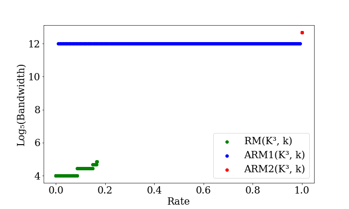
The ARM codes will have greater repair bandwidth than the RM codes when qq increases. However, the expression of the bandwidth makes it difficult to immediately appreciate the improvement in rate gained by implementing the ARM codes. Figure 5 graphs the rate versus the repair bandwidth of the repair schemes of RM​(𝔽543,k)\textrm{RM}(\mathbb{F}_{5^{4}}^{3},k), ARM1​(𝔽543,k)\textrm{ARM1}(\mathbb{F}_{5^{4}}^{3},k), and ARM2​(𝔽543,k),\textrm{ARM2}(\mathbb{F}_{5^{4}}^{3},k), for all values of kk where the repair schemes developed in [7, Theorem 1] and Corollary 4.3 can be applied. The same figure demonstrates that RM codes admit repair schemes with much lower bandwidth than the ARM. However, it also reveals that the ARM codes have significantly higher rates, increasing from at most 0.20.2 to more than 0.990.99. Actual values can be found in Examples 6.4 and 6.5.
Refer to caption
Figure 5. Rate versus the repair bandwidth of the repair schemes of RM​(𝔽543,k)\textrm{RM}(\mathbb{F}_{5^{4}}^{3},k), ARM1​(𝔽543,k)\textrm{ARM1}(\mathbb{F}_{5^{4}}^{3},k), and ARM2​(𝔽543,k),\textrm{ARM2}(\mathbb{F}_{5^{4}}^{3},k), for all values of kk where the repair schemes developed in [7, Theorem 1] and Corollary 4.3 can be applied.
Example 6.4.

Let q=5q=5, t=4t=4, and m=3.m=3. The maximum kk for which RM​(Km,k)\textrm{RM}(K^{m},k) admits the repair scheme given in [2, Theorem III.1] is 623.623. The maximum kk for which ARM1​(Km,k)\textrm{ARM1}(K^{m},k) and ARM2​(Km,k)\textrm{ARM2}(K^{m},k) admit the repair scheme given in Corollary 4.3 is 499.499. The code RM​(Km,623)\textrm{RM}(K^{m},623) has rate 0.1670.167 and bandwidth 24962496. The code ARM1​(Km,499)\textrm{ARM1}(K^{m},499) has rate 0.9920.992 and bandwidth 245312496245312496. The code ARM2​(Km,499)\textrm{ARM2}(K^{m},499) has rate 0.9999984680.999998468 and bandwidth 245312496245312496.

Example 6.5.

The maximum kk for which RM​(𝔽275,k)\textrm{RM}(\mathbb{F}_{2^{7}}^{5},k) admits the repair scheme given in [2, Theorem III.1] is 126.126. The maximum kk for which ARM1​(𝔽275,k)\textrm{ARM1}(\mathbb{F}_{2^{7}}^{5},k) and ARM2​(𝔽275,k)\textrm{ARM2}(\mathbb{F}_{2^{7}}^{5},k) admit the repair scheme given in Corollary 4.3 is 63.63. The code RM​(𝔽275,126)\textrm{RM}(\mathbb{F}_{2^{7}}^{5},126) has rate 0.0090023760.009002376 and bandwidth 889889. The code ARM1​(𝔽275,62)\textrm{ARM1}(\mathbb{F}_{2^{7}}^{5},62) has rate 0.969750.96975 and bandwidth 3597035109735970351097. The code ARM2​(𝔽275,k)\textrm{ARM2}(\mathbb{F}_{2^{7}}^{5},k) has rate 0.9999999910.999999991 and bandwidth 3597035109735970351097.

Previous examples support the same conclusion. Reed-Muller codes admit repair schemes with superior bandwidth but have massively inferior rates when compared with the augmented codes.

We now compare augmented Reed-Muller and Cartesian codes when the length and the field 𝔽qt\mathbb{F}_{q^{t}} are both fixed.

Example 6.6.

Assume that an augmented code of length n>8n>8 over the field 𝔽23\mathbb{F}_{2^{3}} is required. The augmented Reed-Muller code with minimum length greater than 88 is the code ARM1​(𝔽232,k),\textrm{ARM1}(\mathbb{F}_{2^{3}}^{2},k), where 0≤k≤4.0\leq k\leq 4. The bandwidth is b=|K|m−1+(t−1)​(|K|m−1−1)=82−1+(2)​(8−1)=77.b=|K|^{m}-1+(t-1)(|K|^{m-1}-1)=8^{2}-1+(2)(8-1)=77. The augmented Cartesian code with minimum length greater than 88 is the code ACar1​(S1×S2,(k1,k2)),\textrm{ACar1}(S_{1}\times S_{2},(k_{1},k_{2})), where n1=|S1|=4,n_{1}=|S_{1}|=4, n2=|S2|=8,n_{2}=|S_{2}|=8, k1=0k_{1}=0 and 0≤k2≤4.0\leq k_{2}\leq 4. The bandwidth is b=∏i=1mni−1+(t−1)​(∏i=1m−1ni−1)=(4)​(8)−1+(2)​(4−1)=37.b=\prod_{i=1}^{m}n_{i}-1+(t-1)\left(\prod_{i=1}^{m-1}n_{i}-1\right)=(4)(8)-1+(2)(4-1)=37.

Finally we study the case when Reed-Solomon, Reed-Muller and augmented Reed-Muller codes achieve their maximum rate.

6.1. Maximum rates and asymptotic behavior

Focusing on the improved rate, here we study the asymptotic behavior of the rate and the bandwidth rate bn​t,\displaystyle\frac{b}{nt}, which represents the fraction of the codeword that is needed by the repair scheme to recover the erased symbol. We continue with the notation K=𝔽qt.K=\mathbb{F}_{q^{t}}.

Reed-Solomon The maximum kk for which RS​(K,k)\textrm{RS}(K,k) admits the repair scheme given in [7, Theorem 1] is k∗=qt−qt−1.k^{*}=q^{t}-q^{t-1}. On this case, dimKRS​(K,k)=qt−qt−1\dim_{K}\textrm{RS}(K,k)=q^{t}-q^{t-1} and the bandwidth at k∗k^{*} is b∗=(qt−1).b^{*}=(q^{t}-1). Thus

limt→∞dimKRS​(K,k)n\displaystyle\lim_{t\to\infty}\frac{\displaystyle\dim_{K}\textrm{RS}(K,k)}{n} =\displaystyle= limt→∞qt−qt−1qt−1=limt→∞qt−1​(q−1)qt−1​(q−1qt)=1−1q.\displaystyle\lim_{t\to\infty}\frac{q^{t}-q^{t-1}}{q^{t}-1}=\lim_{t\to\infty}\frac{q^{t-1}(q-1)}{q^{t-1}(q-\frac{1}{q^{t}})}=1-\frac{1}{q}.
limt→∞Bandwidtht​n\displaystyle\lim_{t\to\infty}\frac{\text{Bandwidth}}{tn} =\displaystyle= limt→∞qt−1t⁡(qt−1)=limt→∞1t=0.\displaystyle\lim_{t\to\infty}\frac{q^{t}-1}{t(q^{t}-1)}=\lim_{t\to\infty}\frac{1}{t}=0.

Reed-Muller The maximum kk for which RM​(Km,k)\textrm{RM}(K^{m},k) admits the repair scheme given in [2, Theorem III.1] is k∗=qt−2.k^{*}=q^{t}-2. On this case, dimKRM​(Km,k∗)=(m+qt−2qt−2)\dim_{K}\textrm{RM}(K^{m},k^{*})=\displaystyle{m+q^{t}-2\choose q^{t}-2} and bandwidth at k∗k^{*} is b∗=(qt−1)​t.b^{*}=(q^{t}-1)t. Thus

limt→∞dimKRM​(Km,k∗)n\displaystyle\lim_{t\to\infty}\frac{\displaystyle\dim_{K}\textrm{RM}(K^{m},k^{*})}{n} =\displaystyle= limt→∞(m+qt−2qt−2)qt​m\displaystyle\lim_{t\to\infty}\frac{\displaystyle{m+q^{t}-2\choose q^{t}-2}}{\displaystyle q^{tm}}
=\displaystyle= limt→∞(m+qt−2)!(qt−2)!​m!​qt​m\displaystyle\lim_{t\to\infty}\frac{\left(m+q^{t}-2\right)!}{\left(q^{t}-2\right)!\,\,m!\,\,q^{tm}}
=\displaystyle= limt→∞(qt−2+1)⋯(qt−2+m)m!​qt​m=1m!.\displaystyle\lim_{t\to\infty}\frac{\left(q^{t}-2+1\right)\cdots\left(q^{t}-2+m\right)}{m!\,\,q^{tm}}=\frac{1}{m!}\,.
limt→∞Bandwidtht​n\displaystyle\lim_{t\to\infty}\frac{\text{Bandwidth}}{tn} =\displaystyle= limt→∞(qt−1)​tt​qt​m=limt→∞qt−1qt​m=0.\displaystyle\lim_{t\to\infty}\frac{(q^{t}-1)t}{tq^{tm}}=\lim_{t\to\infty}\frac{q^{t}-1}{q^{tm}}=0.

Augmented Reed-Muller 1 The maximum kk for which ARM1​(Km,k)\textrm{ARM1}(K^{m},k) admits the repair scheme given in Corollary 4.3 is k∗=qt−qt−1.k^{*}=q^{t}-q^{t-1}. On this case, dimKARM1​(Km,k∗)=qt​m−q(t−1)​m\dim_{K}\textrm{ARM1}(K^{m},k^{*})=q^{tm}{-}q^{(t-1)m} and bandwidth at k∗k^{*} is b∗=|K|m−1+(t−1)​(|K|m−1−1).b^{*}=|K|^{m}-1+(t-1)(|K|^{m-1}-1). Thus

limt→∞dimKARM1​(Km,k∗)n\displaystyle\lim_{t\to\infty}\frac{\dim_{K}\textrm{ARM1}(K^{m},k^{*})}{n} =\displaystyle= limt→∞qt​m−q(t−1)​mqt​m=1−1qm.\displaystyle\lim_{t\to\infty}\frac{q^{tm}{-}q^{(t-1)m}}{q^{tm}}=1-\frac{1}{q^{m}}\,.
limt→∞Bandwidthn​t\displaystyle\lim_{t\to\infty}\frac{\text{Bandwidth}}{nt} =\displaystyle= limt→∞qt​m−1+(t−1)​(qt⁡(m−1)−1)t​qt​m\displaystyle\lim_{t\to\infty}\frac{q^{tm}-1+(t-1)(q^{t(m-1)}-1)}{tq^{tm}}
=\displaystyle= limt→∞[qt​m−1t​qt​m+(t−1)​(qt⁡(m−1)−1)t​qt​m]=0.\displaystyle\lim_{t\to\infty}\left[\frac{q^{tm}-1}{tq^{tm}}+\frac{(t-1)(q^{t(m-1)}-1)}{tq^{tm}}\right]=0.

Augmented Reed-Muller 2 The maximum kk for which ARM2​(Km,k)\textrm{ARM2}(K^{m},k) admits the repair scheme given in Corollary 4.3 is k∗=qt−qt−1.k^{*}=q^{t}-q^{t-1}. On this case, dimKARM2​(Km,k∗)=qt​m−m⁡(qt−1−1)−1\dim_{K}\textrm{ARM2}(K^{m},k^{*})=q^{tm}{-}m(q^{t-1}-1)-1 and bandwidth at k∗k^{*} is b∗=|K|m−1+(t−1)​(|K|m−1−1).b^{*}=|K|^{m}-1+(t-1)(|K|^{m-1}-1). Thus

limt→∞dimKARM2​(Km,k∗)n\displaystyle\lim_{t\to\infty}\frac{\dim_{K}\textrm{ARM2}(K^{m},k^{*})}{n} =\displaystyle= limt→∞qt​m−m​qt−1+m−1qt​m\displaystyle\lim_{t\to\infty}\frac{q^{tm}{-}mq^{t-1}+m-1}{q^{tm}}
=\displaystyle= limt→∞1−mqt⁡(m−1)+1+m−1qt​m=1.\displaystyle\lim_{t\to\infty}1-\frac{m}{q^{t(m-1)+1}}+\frac{m-1}{q^{tm}}=1.
limt→∞Bandwidthn​t\displaystyle\lim_{t\to\infty}\frac{\text{Bandwidth}}{nt} =\displaystyle= limt→∞qt​m−1+(t−1)​(qt⁡(m−1)−1)t​qt​m\displaystyle\lim_{t\to\infty}\frac{q^{tm}-1+(t-1)(q^{t(m-1)}-1)}{tq^{tm}}
=\displaystyle= limt→∞[qt​m−1t​qt​m+(t−1)​(qt⁡(m−1)−1)t​qt​m]=0.\displaystyle\lim_{t\to\infty}\left[\frac{q^{tm}-1}{tq^{tm}}+\frac{(t-1)(q^{t(m-1)}-1)}{tq^{tm}}\right]=0.

Augmented Cartesian Codes The maximum 𝒌∗\bm{k}^{*} for which ACar1​(𝒮,𝒌∗)\textrm{ACar1}(\mathcal{S},\bm{k}^{*}) admits the repair scheme given in Corollary 4.2 is ki∗=ni−qt−1.k^{*}_{i}=n_{i}-q^{t-1}. On this case, dimACar1​(𝒮,𝒌∗)=∏j=1mnj−∏j=1m(nj−kj)\dim\textrm{ACar1}(\mathcal{S},{\bm{k}}^{*})=\prod_{j=1}^{m}n_{j}-\prod_{j=1}^{m}(n_{j}-k_{j}) and bandwidth at 𝒌∗{\bm{k}}^{*} is b∗=∏i=1mni−1+(t−1)​(∏i=1m−1ni−1).b^{*}=\prod_{i=1}^{m}n_{i}-1+(t-1)\left(\prod_{i=1}^{m-1}n_{i}-1\right). Thus

limt→∞Bandwidthn​t\displaystyle\lim_{t\to\infty}\frac{\textrm{Bandwidth}}{nt} =limt→∞∏i=1mni−1+(t−1)​(∏i=1m−1ni−1)t​∏i=1mni\displaystyle=\lim_{t\to\infty}\frac{\prod_{i=1}^{m}n_{i}-1+(t-1)(\prod_{i=1}^{m-1}n_{i}-1)}{t\prod_{i=1}^{m}n_{i}}
=limt→∞∏i=1mni−1t​∏i=1mni+t−1t​(∏i=1m−1ni∏i=1mni−1∏i=1mni)\displaystyle=\lim_{t\to\infty}\frac{\prod_{i=1}^{m}n_{i}-1}{t\prod_{i=1}^{m}n_{i}}+\frac{t-1}{t}\left(\frac{\prod_{i=1}^{m-1}n_{i}}{\prod_{i=1}^{m}n_{i}}-\frac{1}{\prod_{i=1}^{m}n_{i}}\right)
=limt→∞∏i=1mni−1t​∏i=1mni+t−1t​(1nm−1∏i=1mni).\displaystyle=\lim_{t\to\infty}\frac{\prod_{i=1}^{m}n_{i}-1}{t\prod_{i=1}^{m}n_{i}}+\frac{t-1}{t}\left(\frac{1}{n_{m}}-\frac{1}{\prod_{i=1}^{m}n_{i}}\right).

In the case where nm=𝒪⁡(t)n_{m}=\mathcal{O}(t), we have that this limit is 00.

Now we will discuss the limit of the rate of an Augmented Cartesian Code 1 as the extension degree tt approaches infinity through examples. We will find that varying the Cartesian evaluation set will result in augmented Cartesian codes with rate limits varying between 00 and 1−1qm1-\frac{1}{q^{m}}, even when taking the maximum allowable kjk_{j}’s.

Example 6.7.

Suppose we are in the case when the evaluation set 𝒮=S1×⋯×Sm\mathcal{S}=S_{1}\times\cdots\times S_{m} is such that nj=qt−1+1n_{j}=q^{t-1}+1 for all j∈[m].j\in[m]. Consider the augmented Cartesian 1 code ACar1​(𝒮,𝒌∗)\textrm{ACar1}(\mathcal{S},\bm{k}^{*}) with maximum rate. This happens when 𝒌∗=𝟏.\bm{k}^{*}=\bm{1}. The limit of the rate of this code as tt approaches infinity is

limt→∞dimKACar1​(𝒮,𝟏)n\displaystyle\lim_{t\to\infty}\frac{\dim_{K}\textrm{ACar1}(\mathcal{S},\bm{1})}{n} =limt→∞∏i=1mni−∏i=1m(ni−ki)∏i=1mni\displaystyle=\lim_{t\to\infty}\frac{\prod_{i=1}^{m}n_{i}-\prod_{i=1}^{m}(n_{i}-k_{i})}{\prod_{i=1}^{m}n_{i}}
=limt→∞(qt−1+1)m−(qt−1)m(qt−1+1)m=0.\displaystyle=\lim_{t\to\infty}\frac{(q^{t-1}+1)^{m}-(q^{t-1})^{m}}{(q^{t-1}+1)^{m}}=0.
Example 6.8.

Suppose we are in the case when the evaluation set 𝒮=S1×⋯×Sm\mathcal{S}=S_{1}\times\cdots\times S_{m} is such that ni=qt−1n_{i}=q^{t-1} for i∈[m−1]i\in[m-1] and nm=2​qt−1.n_{m}=2q^{t-1}. Consider the augmented Cartesian 1 code ACar1​(𝒮,𝒌∗)\textrm{ACar1}(\mathcal{S},\bm{k}^{*}) with maximum rate. This happens when ki∗=0k_{i}^{*}=0 for i∈[m−1]i\in[m-1] and km∗=qt−1.k^{*}_{m}=q^{t-1}. The limit of the rate of this code as tt approaches infinity is

limt→∞dimKACar1​(𝒮,𝒌)n\displaystyle\lim_{t\to\infty}\frac{\dim_{K}\textrm{ACar1}(\mathcal{S},\bm{k})}{n} =limt→∞∏i=1mni−∏i=1m(ni−ki)∏i=1mni\displaystyle=\lim_{t\to\infty}\frac{\prod_{i=1}^{m}n_{i}-\prod_{i=1}^{m}(n_{i}-k_{i})}{\prod_{i=1}^{m}n_{i}}
=limt→∞1−∏i=1mqt−12​∏i=1mqt−1=1−12=12.\displaystyle=\lim_{t\to\infty}1-\frac{\prod_{i=1}^{m}q^{t-1}}{2\prod_{i=1}^{m}q^{t-1}}=1-\frac{1}{2}=\frac{1}{2}.
Example 6.9.

Lastly, consider the case when |S|=Km|S|=K^{m}. As this is an augmented Reed-Muller code, we obtain

limt→∞dimKACar1​(𝒮,𝒌)n=limt→∞qt​m−q(t−1)​mqt​m=1−1qm.\displaystyle\lim_{t\to\infty}\frac{\dim_{K}\textrm{ACar1}(\mathcal{S},\bm{k})}{n}=\lim_{t\to\infty}\frac{q^{tm}{-}q^{(t-1)m}}{q^{tm}}=1-\frac{1}{q^{m}}.

A similar situation happens with the augmented Cartesian codes 2. We summarize these findings in Table 1.

Code Dimension limt→∞Rate\displaystyle\lim_{t\to\infty}\text{Rate} limt→∞b∗n​t\displaystyle\lim_{t\to\infty}\frac{\displaystyle b^{*}}{nt}
RS​(K,m​a​x)\textrm{RS}(K,max) qt−qt−1q^{t}-q^{t-1} 1−1q\displaystyle 1-\frac{1}{q} 00
RM​(Km,m​a​x)\textrm{RM}(K^{m},max) (m+qt−2qt−2)\displaystyle{m+q^{t}-2\choose q^{t}-2} 1m!\displaystyle\frac{1}{m!} 00
ARM1​(Km,m​a​x)\textrm{ARM1}(K^{m},max) qt​m−q(t−1)​mq^{tm}{-}q^{(t-1)m} 1−1qm\displaystyle 1-\frac{1}{q^{m}} 00
ARM2​(Km,m​a​x)\textrm{ARM2}(K^{m},max) qt​m−m⁡(qt−1−1)−1q^{tm}{-}m(q^{t-1}{-}1){-}1 11 00
ACar1​(𝒮,m​a​x)\textrm{ACar1}({\bf\mathcal{S}},max) ∏j=1mnj−∏j=1m(nj−kj)\displaystyle\prod_{j=1}^{m}n_{j}-\displaystyle\prod_{j=1}^{m}(n_{j}-k_{j}) b/w 0−10-1 00
ACar2​(𝒮,m​a​x)\textrm{ACar2}({\bf\mathcal{S}},max) ∏i=1mni−∑i=1m(ni−ki−1)−1\displaystyle\prod_{i=1}^{m}n_{i}-\displaystyle\sum_{i=1}^{m}(n_{i}-k_{i}-1)-1 b/w 0−10-1 00
Table 1. Asymptotic behavior of the RS,RM,ARM1\textrm{RS},\textrm{RM},\textrm{ARM1} and ARM2,\textrm{ARM2}, when each achieves the maximum dimension so the associated repair scheme can be applied. The number b∗n​t\displaystyle\frac{b^{*}}{nt} represents the fraction of the codeword that is needed by the repair scheme to recover an erased symbol.

As expected, the augmented codes, which were designed to maximize the rate of the code, have a higher repair bandwidth as well, due to the trade-off between the rate of a code and the bandwidth of its associated repair scheme. In the end, neither of these schemes is objectively better than the other. Any potential user should opt to use the scheme that best deals with the parameter most important to their application, whether that be one that requires high rate codes or one that requires low bandwidth recovery.

7. Conclusions

In this paper, we introduce a new family of evaluation codes, called augmented Cartesian codes, along with repair schemes for single and certain multiple erasures. They can be designed to have higher rate than their traditional counterparts and include as a special case augmented Reed-Muller codes. In some circumstances, these repair schemes may have lower bandwidth and bitwidth than comparable algebraic geometry codes (such as Reed-Solomon or Hermitian codes). There are parameter ranges in which repairing Reed-Solomon codes may not be available, such as dimension between qt−qt−1q^{t}-q^{t-1} and qtq^{t} over 𝔽qt\mathbb{F}_{q^{t}}. In some cases, augmented Reed-Muller codes may be designed along with repair schemes for single or pairs of erasures. More generally, we can use augmented Cartesian codes to provide high-rate codes with repair schemes for single erasures and certain pairs of erasures in those settings where the augmented Reed-Muller codes are not.

References

  • [1] E. Camps, H. H. López, G. L. Matthews and E. Sarmiento, Polar Decreasing Monomial-Cartesian Codes, IEEE Transactions on Information Theory, 67 (2021), no. 6, 3664–3674.
  • [2] T. Chen and X. Zhang, Repairing Generalized Reed-Muller Codes, https://arxiv.org/pdf/1906.10310.pdf.
  • [3] P. Delsarte, J. M. Goethals and F. J. Mac Williams, On generalized Reed-Muller codes and their relatives, Information and control, 16 (1970), no. 5, 403–442.
  • [4] A. Dimakis, P. Godfrey, Y. Wu, M. Wainwright and K. Ramchandran, Network coding for distributed storage systems, IEEE Transactions on Information Theory, 56 (2010), no. 9, 4539–4551.
  • [5] A. Dimakis, K. Ramchandran, Y. Wu and C. Suh, A survey on network codes for distributed storage, Proceedings of the IEEE, 99 (2011), no. 3, 476–489.
  • [6] O. Geil, and C. Thomsen, Weighted Reed-Muller codes revisited, Designs Codes and Cryptography, 66 (2013), 195–220. https://doi.org/10.1007/s10623-012-9680-8
  • [7] V. Guruswami and M. Wootters, Repairing Reed-Solomon Codes, IEEE Transactions on Information Theory, 63 (2017), no. 9, 5684–5698.
  • [8] W. C. Huffman and V. Pless, Fundamentals of error-correcting codes, Cambridge University Press, Cambridge, 2003.
  • [9] D. Jaramillo, M. Vaz Pinto, and R. H. Villarreal, Evaluation codes and their basic parameters, Designs Codes and Cryptography, 89 (2021), 269–300.
  • [10] L. Jin, Y. Luo and C. Xing, Repairing Algebraic Geometry Codes, IEEE Transactions on Information Theory, 64 (2018), no. 2, 900–908.
  • [11] H. H. López, G. L. Matthews and I. Soprunov, Monomial-Cartesian codes and their duals, with applications to LCD codes, quantum codes, and locally recoverable codes, Designs Codes and Cryptography, 88 (2020), 1673–1685.
  • [12] H. H. López, G. L. Matthews and D. Valvo, Augmented Reed-Muller Codes of High Rate and Erasure Repair, Proceedings of the IEEE, (2021), to appear.
  • [13] H. H. López, C. Rentería-Márquez and R. H. Villarreal, Affine Cartesian codes, Designs, Codes and Cryptography 71 (2014), no. 1, 5–19.
  • [14] H. H. López, I. Soprunov and R. H. Villarreal, The dual of an evaluation code, Designs, Codes and Cryptography, (2021), https://doi.org/10.1007/s10623-021-00872-w.
  • [15] H. Dau, I. Duursma, H. Kiah and O. Milenkovic, Repairing Reed-Solomon Codes With Multiple Erasures, IEEE Transactions on Information Theory, 64 (2018), no. 10, 6567–6582.
  • [16] R. Lidl and H. Niederreiter, Introduction to finite fields and their applications, Cambridge University Press (1994), https://doi.org/10.1017/CBO9781139172769.