Optimality Inductive Biases and Agnostic Guidelines for Offline Reinforcement Learning
Abstract
The performance of state-of-the-art offline RL methods varies widely over the spectrum of dataset qualities, ranging from far-from-optimal random data to close-to-optimal expert demonstrations. We re-implement these methods to test their reproducibility, and show that when a given method outperforms the others on one end of the spectrum, it never does on the other end. This prevents us from naming a victor across the board. We attribute the asymmetry to the amount of inductive bias injected into the agent to entice it to posit that the behavior underlying the offline dataset is optimal for the task. Our investigations confirm that careless injections of such optimality inductive biases make dominant agents subpar as soon as the offline policy is sub-optimal. To bridge this gap, we generalize importance-weighted regression methods that have proved the most versatile across the spectrum of dataset grades into a modular framework that allows for the design of methods that align with how much we know about the dataset. This modularity enables qualitatively different injections of optimality inductive biases. We show that certain orchestrations strike the right balance, improving the return on one end of the spectrum without harming it on the other end. While the formulation of guidelines for the design of an offline method reduces to aligning the amount of optimality bias to inject with what we know about the quality of the data, the design of an agnostic method for which we need not know the quality of the data beforehand is more nuanced. Only our framework allowed us to design a method that performed well across the spectrum while remaining modular if more information about the quality of the data ever becomes available.
1 Introduction
Reinforcement learning (RL) [134] is the branch of interactive machine learning that has received the most attention in recent years, due to its instrumental role in tackling a number of grand AI challenges (e.g. going beyond human performance in board and video games [83, 84, 126, 125, 148, 93], hitting a new milestone in AI-operated hand dexterity leading to the resolution of a Rubik’s cube [92]). The online RL agents learn by acting in the world (either real or simulated), and update their intrinsic decision-making process by internalizing the feedback returned by the world upon interaction. The feedback takes the form of a reward signal, which scores the agent according to how appropriate its own executed actions were for the task at hand (how rewards are designed or come from is out of the scope of this paper, cf. [129]). Nonetheless, while learning from our mistakes is undeniably valuable, it is of far greater value to be able to learn from the mistakes of others, a sub-branch of machine learning sometimes referred to as counterfactual learning [20]. In the context of RL, pure counterfactual learning crystallizes as offline RL [73] (alternatively, batch RL [70]). The agent is only allowed to learn from an offline dataset. This dataset contains logged interactions that were experienced and collected by another policy as it interacted with the world. The offline RL agent is not allowed to interact with the world, and is consequently unable to learn interactively from her own mistakes.
Offline RL shines a) when interaction data (albeit from multiple non-egocentric sources) are abundant and diverse and b) when simulator-in-the-loop approaches are impractical, due to deterringly high costs or safety concerns. In practice, it is incredibly tedious and challenging to design and implement a data collection strategy able to capture the diversity of the real world in a dataset. Besides, crafting a simulator able to model how the world reacts to the agent with high fidelity is an engineering feat too (e.g. the elaborate system of automatic domain randomization used in [92] to assist in the resolution of of a Rubik’s cube, which required the aid of the purposely-developed asset randomization engine reported in [24]). Iteratively integrating hitherto-omitted edge cases is a long-term endeavor. Even when one manages to train agents yielding high return in simulation, they are not guaranteed to transfer to the real world, and often require additional model surgery (cf. “sim-to-real” research [118], a sub-domain of transfer RL [137]). Designing offline RL methods able to squeeze the most juice out of potentially imperfect offline real-world interaction data is both a crucial and timely problem to solve. The crying need for such methods in popular consumer-facing real-world applications (e.g. robotics, autonomous driving, healthcare, conversational agents) explains the resurgence of offline RL [73].
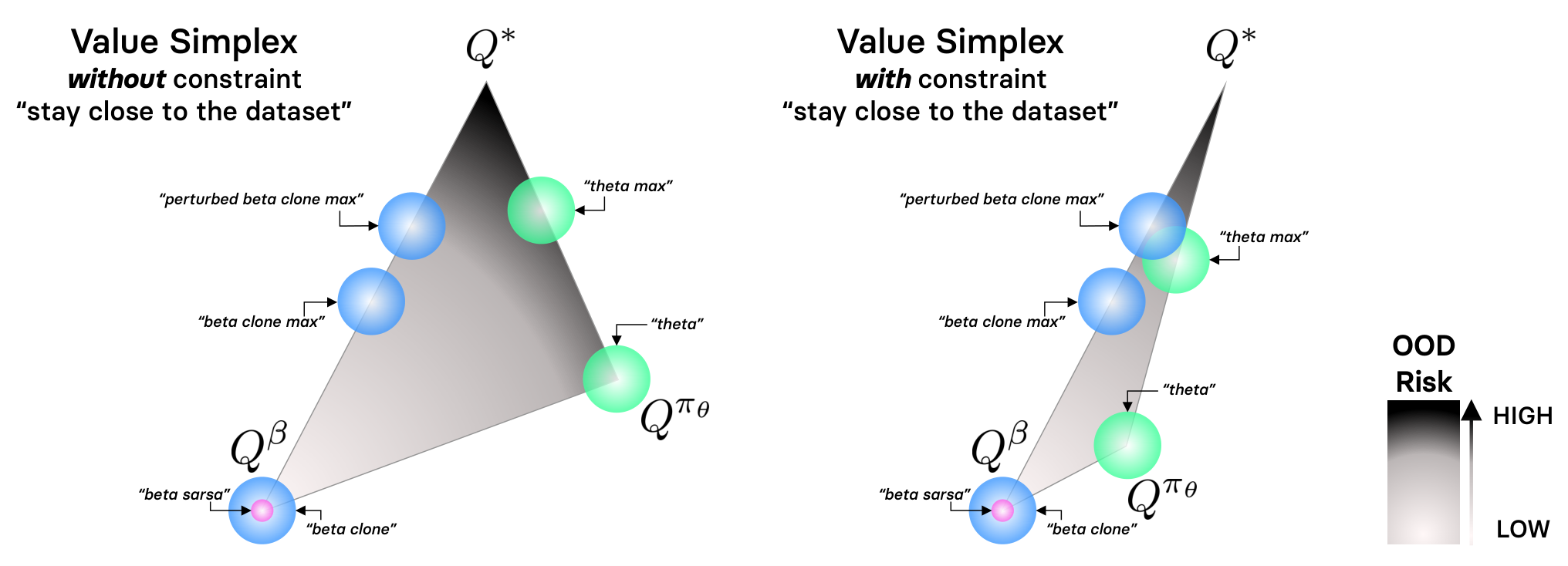
Online off-policy actor-critic methods require the decision-maker to learn an estimate of the state-action value through bootstrapping with next actions generated by the agent, and as such implement the SARSA update rule [116, 140, 133, 147]. These methods suffer from a distributional shift [33] as soon as the experience replay [76] mechanism comes into play, since an action generated by the current policy is used to update the value at an action randomly picked from the replay memory — effectively distributed as a mixture of past policy updates. This covariate shift phenomenon is exacerbated in the offline setting, where the value is only subject to updates at the fixed set of actions present on the offline dataset. Since the distribution over actions underlying the offline dataset neither evolves nor need be tied to the agent’s policy in any way, the distributional shift can grow arbitrarily large. By contrast, the mixture of past policy updates underlying a replay memory will by design always track (yet not necessarily closely) the current policy update, effectively limiting the gap between the action distributions. Since in the offline setting the value is solely updated over a frozen offline dataset detached from the policy followed by the agent, the value is all the more so exposed to being evaluated at out-of-distribution actions than its counterpart in the online (off-policy) setting. As such, the value can be arbitrarily erroneous at actions that are too far off the offline distribution underlying the dataset. This motivates the design of offline RL methods that deter the agent from straying onto out-of-distribution action by urging the agent to “stay close to the offline dataset” (cf. Figure 1), either explicitly or implicitly. We lay these out in Section 3.
2 Contributions
Contribution #1: critical evaluation of the landscape.
We open-source11 1 Code made available at the URL: https://github.com/lionelblonde/giwr-pytorch. fair re-implementations of state-of-the-art offline RL methods under a proposed unified framework. In Section 5.1, we discuss the methods included in this release, before assessing and comparing these competing methods empirically in Section 5.2. This study, along with all the other analyses reported in this work, are conducted under the experimental setting laid out in Appendix A.
Contribution #2: optimality inductive biases.
In Section 6.1, we explicitly formalize the notion of optimality inductive bias. When injected into the decision-maker, it conceptually quantifies how much the latter posits that the policy underlying the offline dataset is optimally solving the task at hand. We investigate empirically to what extent the amount of inductive bias injected in the agent impacts its performance across the spectrum of considered datasets and environments. The performance comparison depicted in Section 5.2 shows how most baselines inject far too much optimality inductive bias to achieve reasonable levels of performance when the dataset is sub-optimal. Besides, these baselines have proven hard to tune [157, 72, 85], and the hyper-parameters displaying the largest swings in performance are the ones controlling the amount of bias injected. From Section 6 forward, we use the advantage-weighted regression template (cf. Algorithm 1) adopted identically in [152] and [88], given that it yields the most favorable empirical results in Section 5.2. In order to verify that its competitive superiority over the spectrum of dataset qualities is due to the implicit nature of how such agents are injected with optimality inductive bias, we construct and diagnose an extension of the base advantage-weighted regression method in Section 6.2. We handcraft this extension by regularizing the optimized objective such that the extension injects more optimality inductive bias into the agents trained with it than the base method does. We push the diagnostic further by evaluating the return of both methods, for a given environment, on a series of mixed datasets each simulating a scenario in which the expert dataset has been corrupted with transitions from the random dataset, to various degrees of severity. These reveal just how strikingly sensitive to the means of bias injection offline RL methods are, especially considering how often real-world data is corrupted.
Contribution #3: Generalized Policy Iteration (GPI) revisitation for offline RL, leading to the novel Generalized Importance-Weighted Regression (GIWR) framework.
In Sections 7, 8 and 9, we propose generalizations of the value and policy objectives involved in the considered base actor-critic method (cf. Algorithm 1), where Section 7 primarily aims at setting the stage for both of the subsequent remaining sections. Section 8 is dedicated to policy evaluation, and Section 9 is dedicated to policy improvement. These generalizations involve proposal policies, effectively acting as placeholders for a slew of different action distributions that we introduce (9 in total) and evaluate, in both contexts (evaluation in Section 8, improvement in Section 9). Each proposal strategy tackles, with its own distinct flavor, the balancing act that both the policy and value entangled in a GPI scheme must address in offline RL: how to come close to behaving optimally for the given task while avoiding being hindered by out-of-distribution actions? Under a notion of safety purposely derived from this desideratum, we can equivalently ask: how to teach offline agents to approach optimality safely? As illustrated in Figure 1, striking the right balance is far from obvious and highly dependent on the quality of the dataset. Nonetheless, we show that our new, highly modular, generalized framework (we call it GIWR, which stands for Generalized Importance-Weighted Regression, cf. Section 9.3) enables us to safely inject optimality inductive bias(es) in the method in such a way that the results are improved when the policy underlying the dataset is optimal, while not being harmed when it is not.
N.B.
Our agents are never made aware of the quality of the offline dataset they are provided with.

3 Related Work
The subfield of offline RL has been outlined in two surveys, under slightly different scopes. In [70], the authors give an overview of the batch setting, and a thorough picture of how it was tackled from its inception by Gordon in 1995 (cf. [39]) to the release date of the survey. Eight years later, in [73], the offline RL landscape is painted by the authors through a more practice-oriented lens. While [70] identified stability as the main culprit hindering the wide adoption of offline RL in real-world systems (defending that a genuine expertise was needed to pull it off), [73] can depict a more optimistic view of the domain since it has since received attention and been leveraged in various applications (e.g. such as dialog systems). Despite having been addressed numerous times in recent years, and approached via different angles, the practical stability issues discussed in [70] have yet to be solved, and are barely mitigated in the current state-of-the-art methods. Going back to the inception of batch RL, the work of [39] proposes a model-based method called Averagers that estimates the action-value exactly at supports. It does so by leveraging the exact dynamic programming operation, requiring the availability of a model of the transition function to be able to solve the subsequent planning task with it. Besides, the approach of [39] identifies as a “fitted” one, since it solves the action-value estimation problem before deriving a control policy from it. Note, the sequence diagrams depicted in Figure 1 do not temporally represent the learning process of agents learned under said fitted paradigm — otherwise, the dotted arrows would reach the solid lines every single time. Albeit raised and discussed, [39] did not propose a model-free counterpart of the method, due to convergence issues for estimating the action-values at the supports from the action-values estimated at samples from the respective neighborhoods of the supports. Ormoneit and Sen [94] address this issue, though not in the Averagers framework. Instead of attempting to estimate the values from neighboring samples at supports, they estimate the value directly via a sample-based approximator (which is kernel-based). In other words, instead of relying on a transition model and carrying out the exact dynamic programming operation with it, their Kernel-based Approximate Dynamic Programming (KADP) method detaches itself from the need to possess a model of the world: it approximates the exact dynamic programming operator with the implicit sample-based transition model observable via the collected transitions in the batch (that we have access to, yet ignore the underlying dynamics and behavior models of). Our work is closer to the Least-Squares Policy Iteration (LSPI) method from [68] — whose first release was concurrent with KADP, since we set out to revisit the generalized policy iteration learning template in the offline regime (cf. Section 1 for what motivates our study, cf. Figure 1 for a conceptual depiction of the learning scheme). As such, we only consider methods that alternate between policy evaluation and policy improvement steps, in contrast with the distinct separation of these two problems that characterizes the fitted methods [39, 30, 112, 7, 90, 69, 46]. Note, LSPI [68] does not involve an explicit policy, the policy is defined implicitly from the learned value.
When it comes down to the modern state-of-the-art offline RL approaches which we critically evaluate in this work, one can divide them up into three distinct categories. These differ by how they encode the constraint enticing the agent to stay close to the offline dataset. They do so 1) with explicit constraints on the policy (e.g. BRAC [157], BEAR [66], WOP [52]), or 2) with explicit constraints on the value (e.g. BRAC [157], CQL [67]), or 3) with implicit constraints on the policy (e.g. BC [105, 106, 109, 8] BCQ [34], MARWIL [151], AWR [99], ABM [124], CRR [152], AWAC [88]). Note, we here only list out the model-free approaches — we will discuss the model-based ones momentarily. Optimizing an objective subjected to an implicit constraint corresponds to optimizing a reduction of an objective constrained explicitly. After reduction (e.g. via the Lagrangian method, with KKT conditions assumed to be satisfied in case of inequality constraint) the optimization problem is not constrained anymore, but it is still derived from an explicitly constrained problem, hence the “implicit” denomination. The derivation from a constrained objective to the unconstrained one optimized in MARWIL [151], AWR [99], ABM [124], CRR [152], and AWAC [88] is laid out (albeit under a generalized form) in Section 9. Seeing BCQ [34] as a perturbed, more sophisticated extension of BC, itself consisting in maximizing the likelihood of the learned policy over the data, we can equivalently interpret the objective of these algorithms as the minimization of the forward KL divergence between the true data distribution and the learned policy. As such, we can see these (BC and BCQ) as implicitly constrained.
Pretraining with offline datasets has been studied extensively in recent years. The pursued goal is simply to leverage offline datasets so as to increase the learning speed and final performance of downstream tasks in online RL, imitation learning [8], and even offline RL (with a distinct task however). Such desideratum is pursued notably in [158], [4], [128], and [88]. Nonetheless, we are not interested in this type of bootstrap and transfer capabilities in this work.
The endeavors we carry out in Section 8, including the formulation of the proposal action distributions (from which the next actions are to be sampled) relate to a slew of works that also attempted to skew the SARSA variant of Bellman’s equation (used in usual actor-critic’s) towards the optimal variant of Bellman’s equation (used in Q-learning [153, 154]). Although plenty of modifications to the Bellman operator have been proposed throughout the years to entice the policy and value to adopt a certain desired behavior, we are here only interested in approaching the optimal action-value. The discussion that follows therefore focuses on how previous works have successfully been able to inject bias towards the optimal behavior in their respective agents. We align the notion of optimality with Bellman’s principle of optimality. As such, a policy is optimal if and only if its value is solution to the optimal version of Bellman’s equation. Whether an expert dataset (possibly human-generated) should be considered optimal is a valid question — discussed in [117]. While one can just substitute the SARSA operator with the Q-learning one when dealing with discrete actions (cf. [25] for the a priori earliest adoption of such substitution in an actor-critic), how to proceed in continuous action spaces is less obvious (the operation over actions creates an extra inner-loop optimization problem to solve every iteration). Different approaches have been adopted to circumvent this hindrance. As such, we discern four main strategies to tackle the operation in continuous action spaces: 1) discretizing the continuous action space into a discrete space of tractable dimension, then use Q-learning over the crafted discretized space (e.g. [82, 59, 81]), 2) enforcing a strict structure over the Q-value in a way that facilitates the resolution of said extra inner-loop maximization, as done e.g. in NAF [42], 3) getting rid of the hard operation altogether by using a soft update instead [44], and finally 4) tackling the resolution of inner-loop maximization problem every iteration, despite the leap in computational cost caused by the continuous nature of the action space. Approach 4) has, for instance, been implemented via the use of the derivative-free, black-box, Cross-Entropy Method (CEM) [114, 80] optimizer to estimate the maximizing action for the given state at each step, e.g. in QT-Opt [56, 108], and in the Actor-Expert framework [75]. By contrast, the Amortized Q-learning (AQL) [144] method follows approach 4) by taking inspiration from the amortized inference literature and displays a conceptually simpler formulation. In effect, these methods replace the optimal policy that should in theory be used to generate the next action in the SARSA variant of Bellman’s equation (to obtain the Q-learning variant of Bellman’s equation), by a tractable approximation of it — which we refer to as proposal policy in Section 8. For example, QT-Opt [56, 108] craft said proposal policy as the function that, for the given state, at the given iteration, returns the solution of the inner-loop, per-iteration maximization sub-problem obtained via the CEM [114, 80]. Tractable approximations of intractable policies in continuous action spaces with proposal distributions over actions have also notably been carried out in [50] and [155]. Finally, the most noteworthy method implementing approach 4) is perhaps the operator introduced in EMaQ [38], in the offline regime specifically. As we discuss in Section 8, this operator uses a proposal policy that interpolates between a tractable approximation of the optimal policy estimated via AQL, and an estimated clone of the policy underlying the offline dataset. The framework we propose for policy evaluation in Section 8 subsumes such operator. Finally, the optimality tightening [47] technique also aligns with the optimality desideratum pursued here.
Based on how brittle state-action values estimated via temporal-difference learning are in the offline regime — due to the risk of using out-of-distribution actions for bootstrapping the value, one might want to ensure or even guarantee safer updates. This safety desideratum naturally links offline RL to the line of Safe Policy Improvement (SPI) methods (e.g. [139, 103, 71]), in the online regime. As reminded in SPIBB [71] (SPI by Bootstrapping the Q-value with a Baseline, not with the learned policy), the concept of safety in RL is overloaded to say the least (cf. [37]). Among all the possible hindrances one would desire to be shielded from — parametric (epistemic) uncertainty, internal (aleatoric) uncertainty, interruptibility, exploration in a hazardous environment — SPIBB sets out to design a method that guarantees safety against the potential damages that might be caused by an excessive epistemic uncertainty in the learned models. SPIBB builds on the work of Petrik (cf. [103]), that designs a learning update rule for the actor that analytically guarantees a safe policy improvement, whatever the parameters of the model. Aligning its take on safety with Petrik’s, SPIBB provides its agent access to a dataset as well as to a baseline. For most of their experimental endeavors, the dataset is assumed to be distributed as the baseline. Crucially, that is a condition that need be satisfied for the theory backing SPIBB to hold. Nevertheless, the authors also perform a set of experiments in which this restrictive assumption is relaxed. The relaxed scenario (the dataset was not collected with the baseline) is artificially implemented by replacing the dataset optained from the baseline by a dataset collected by a random policy, while the action bootstrap is still carried out using the baseline. This second setting shares a property we investigate in Section 8: how does detaching the proposal policy used to bootstrap from the policy that carried out the data collection, impact performance. We however do not have access to a baseline safeguard and our proposal policies do not require any extra information; they are solely using the offline dataset (at most). The safe policy improvement rule proposed by SPIBB articulates as follows: when the agent is confident that it can improve upon the baseline, it will use its own learned policy, otherwise it will use the oracle baseline as a fallback. We take inspiration from these to formulate three of our proposal distributions, dubbed safe, and used in Sections 8 and 9. As such, our work therefore also subsumes BRPO [130], which also proposes a learning update aligned with the one introduced in the SPI line of works.
By consistently opting for the safer option when there is a potential risk (based on an estimated measure of uncertainty), SPI methods follow a pessimistic heuristic, conceptually opposing the principle of Optimism in the Face of Uncertainty Learning (OFUL) which are ubiquitous in the Multi-Armed Bandits (MAB) and Online Learning (OL) literature. Note, any optimistic measure can trivially be made pessimistic by composing it with a monotonically decreasing function over reals — and optimistic measures of uncertainty or novelty are plentiful in the MAB, OL, and online RL literature to infuse the agent with exploratory incentives. Nonetheless, considering how the offline agent are unable to learn from their own mistakes (since their interactions are not recorded in the dataset used to train it), encourage exploration by advocating for optimism in the face of uncertainty should be avoided. Research endeavors in offline RL have instead turned to pessimism, as analyzed through a theoretical lens in [22]. Pessimistic modifications to usual algorithms have recurrently been carried out via model-based approaches, consisting in replacing the rewards used by the learning agent with pessimistic reward surrogates. The first occurrence of such technique appears in the RaMDP technique propose by Petrik in [103], where the author also introduced SPI, stressing how both SPI and RaMDP promote the adoption of pessimism when confidence is low. RaMDP transforms the rewards from the dataset via the application of a penalty. A reward from a given transition in the dataset will be penalized less if said transition appears often in the dataset. Conversely, it will be penalized more if the transition appears rarely in the dataset. The frequency of occurrence, used as a measure of confidence, is estimated via a pseudo-count [15, 136, 96]. Years later, MOPO [159] and MoREL [58] concurrently propose virtually identical model-based techniques penalizing the rewards in offline RL. In contrast with RaMDP, they formulate their reward penalties based on the uncertainty of a forward model (aiming to model the inner workings of the MDP). On the topic of reward re-shaping, [70] suggests that using a smoother reward signal might help in stabilizing the learned Q-value, as first proposed and corroborated empirically in [46]. Yet, our preliminary investigation of reward smoothing did not yield improvement for the considered datasets. In this work, we consider only model-free approaches and, like mentioned earlier, dabble in pessimism only via SPI-based techniques.
Finally, the involvement of constraints consisting of KL divergences in the policy improvement objectives discussed and derived in Section 9 echoes the entire “KL-control” line of work, originating in [55, 54, 62, 102, 149, 138, 36, 100, 61, 89, 57]. Honorable mentions that distinguish themselves from these, yet are tightly related, could arguably be G-learning [31], and -learning [110]. In the offline regime, WOP [52] notably implements a KL-control approach.
4 Background
4.1 Setting
In this work, we tackle the problem of offline RL — also sometimes referred to as batch RL [70]: the autonomous agent must learn how to interact optimally in an environment without being allowed to interact with it during training.
On the flip side, our learning agent has access to a collection of interactions (including the received feedback in the form of reward) from another distinct agent. This counterfactual interactive information storage is called the offline dataset, noted . The offline dataset is made available before the learning process starts, and is kept frozen throughout the entirety of the training procedure. Note, we do not consider the “growing batch” setting, in which the dataset can grow during training, either by the hands of the learning agent, or by an external source. Leveraging solely the offline dataset , the agent must learn an online, interactive policy that will enable the accumulation of the high rewards during evaluation phases. Note, we forbid the agent from accessing the offline dataset at evaluation time — allowing it would place our work in the “observational learning” setting. Albeit fairly realistic, we want our agents to be purely online when let loose for evaluation, with no means of tapping into pre-existing repositories of interaction data. As such, our agent uses only the offline dataset without interacting online with its environment at training time, but interacts online with without ever using at evaluation time — neither for reading , nor writing in .
4.2 World and agent
We model as a memoryless, infinite-horizon, and stationary Markov Decision Process (MDP) [107], noted . Formally, , where and are respectively the state space and action space. The dynamics of the world are determined by the stationary, stochastic transition function , and the initial state probability density . In effect, is the conditional probability density concentrated at the state when action is executed in state . The reward feedback that returns upon executing in is modeled as the outcome of a stationary reward process that assigns real-valued rewards distributed as . The remaining piece of is , the discount factor. The decision-making process of the learning agent is modeled by the parametric policy , under a neural representation with the parameter vector . The stochastic policy followed by the agent maps states to probability distributions over actions, which we denote by , or by the compact notation , where . Concretely, the experiences of the agent are divided across discrete timesteps , where . The analyses we carry out in this work do not require the involvement of a finite time horizon , hence our decision to adopt the infinite-horizon MDP setting where is a priori unbounded above in the formalism. Despite being infinite horizon, we make the MDP episodic by assuming that every trace contains at least one absorbing state, and that when the first is reached by the agent, is artificially set to zero to emulate termination, hence formally constructing an episode. At each timestep , the agent is located at , and concentrates a probability density over actions from that is equal to at action . We denote the action selected by the agent’s policy at timestep by , and the received reward by .
Lastly, we introduce the discounted state visitation frequency for an agent following a policy in the MDP , denoted as , and abbreviated in the absence of ambiguity. Formally, , where is the probability of reaching state at timestep ( is a random variable) when following in . Since an immediate derivation gives , can be seen as a probability distribution over states up to a constant factor. Being in the episodic setting, we will use the undiscounted counterpart of , yet still artificially set when the absorbing state (posited earlier to always exist) is reached to emulate episode termination.
4.3 Dataset
We do not have access to the analytical form of the policy that generated the dataset, nor do we have the ability to sample from it. Besides, since none of the approaches mentioned in this work explicitly leverage the fact that the offline dataset might have been produced by multiple distinct sources, we posit w.l.o.g. that the offline dataset contains interaction traces of a single conceptual policy , dubbed the offline distribution. Despite being composed of traces of interaction, these are not necessarily available in connex trajectories, but rather as a shuffled collection of individual transitions. We do not know how the data was collected, in particular what the underlying strategy was optimizing for, nor do we know the proficiency of in satisfying the chased objective other than what we can infer and hopefully extrapolate from the offline dataset. might have been collected with a single fixed snapshot of a policy, in which case is this very snapshot; or might be the training history of a policy, in which case is a mixture of past iterates. For a given dataset , might be focusing on covering the most ground while not paying too much attention to the collected rewards, or conversely covering the least amount of ground while accumulating rewards as greedily as possible. Note, in imitation learning and inverse RL [8] where rewards are not known, one assumes the expert (’s counterpart) was acting optimally when collecting the demonstrations. This is not the case in this work. We use datasets whose quality range from expert-grade data (where is close to optimality) to random data (where wanders seemingly aimlessly) (cf. Appendix A). Our agents are never made aware of ’s quality or ’s proficiency. The offline dataset is formally defined as a collection of SARS-formatted transitions collected by the underlying offline distribution through interactions with . Being in the episodic setting, transitions also contain a termination indicator in practice, taking value when the transition is the last one in the episode, and otherwise. When has a richer structure — from transitions being SARSA-formatted to transitions being sequenced in full connex trajectories — we say so explicitly in the text. As noted in [34] and [71], we have in effect two MDPs in the tackled offline setting: 1) the real, non-observable, online MDP underlying the inaccessible environment , and 2) the fictitious, observable, offline MDP effectively communicated through the dataset to the agent. As such, while interacted with to collect , interacts with — in effect detached from the real world — and collects nothing. Every state in is then distributed as . For legibility purposes, we will use as a shorthand for . In practice, with a slight abuse of notation, we can note to indicate that the transition is in effect obtained by sampling from the offline dataset . Nevertheless, we will often opt for the explicit notation — for SARS-formatted transitions, and for SARSA-formatted transitions — as a drop-in replacement for and , with being replaced by in the operand of the expectation not to overload the notation. We express the reward function as a function of the next state as well, as it is the most general setting and can be reduced to by positing trivial assumptions. We do not indicate the states (and actions when applicable) at which the conditional densities are evaluated in the outer expectations throughout this work, to lighten the notation as much as possible.
4.4 Objective
We here describe the concepts that we need to add to our tool set so as to properly deal with the delayed nature of the reward feedback. In the infinite-horizon regime we placed our agent into, the return is the discounted sum of rewards from timestep onwards, and is at the core of how RL methods attempt to solve the credit assignment problem created by said delayed feedback. We formalize the return of the state-action pair associated with timestep as . The expectation of the return along traces of the arbitrary policy starting from the execution of action in defines the state-action value (also called action-value, or simply Q-value) such as (abbrv. ). We say that a policy acts optimally at timestep if the action selects at state , noted verifies the following identity: . Such behavior coincides with being purely greedy with respect to the exact action-value coupled with (cf. Q-value definition right above). By extension, acts optimally at every timestep if and only if, for any given start state , the policy maximizes . Our objective is for the agent to learn a policy such that is a solution of the optimization problem for any given start state , where is the performance objective (or utility) and is the neural search space for .
4.5 Convenience
KL.
We adopt an alternative notation for the KL divergences by adding an arrow within the operator in order to disambiguate from a quick glance whether it is the forward (inclusive [78]) or the reverse (exclusive [78]) KL divergence, due to its asymmetric nature. The orientation of said arrow indicates the order in which one should write the predicted and target distributions respectively in the original KL divergence notation. As such, denoting the predicted and target distributions as and respectively — the parameter “” being used here to highlight which distribution is parameterized and learned, and which is fixed and set as target — we write, for a given state , to replace , and instead of . With this notation, the target distribution is always indicated in the exponent, of the divergence operator, while the learned distribution to fit to the target is alone in the operand of the operator. By following the arrow, we can then read, without ambiguity, for a given state , a) as “the forward KL between and ”, and b) as “the reverse KL between and ”.
Hyper-parameter stiffness.
Finally, we propose the notion of hyper-parameter stiffness, defined by analogy with the notion of stiff equation in physics: we say that an algorithm is stiff with respect to the hyper-parameter if slight changes in the value of cause large and non-monotonic variations in ’s asymptotic performance, — or, to a more extreme extent, make numerically unstable. In effect, from a practitioner’s perspective, that translates into being tedious to tune. We introduce this notion due to various offline RL methods having been reported for their sensitivity and brittleness w.r.t. hyper-parameter choices — for instance in [72] and [85]. The universal desideratum is to design algorithms that are stiff w.r.t. none of their hyper-parameters , and this is naturally what we aspire to in this work.
5 Critical evaluation of the offline RL landscape
5.1 Experimental setting
As the first contribution of this work, we perform a thorough PyTorch [97] re-implementation of the state-of-the-art competing baselines in offline RL under a common computational infrastructure, and release it as an open-source22 2 Code made available at the URL: https://github.com/lionelblonde/giwr-pytorch. project. This allows not only for meaningful comparisons in which we can vary in a controlled manner different design choices, but also for the easy development of new offline RL algorithms. We lay out a comprehensive exposition of our re-implementations, and the associated design choices we made to ensure their fairness, in Appendix A.1.
We carry out every experiment reported throughout this work in the D4RL suite [32], composed of environment-dataset pairs. We give more details about how we use the suite to carry out our empirical investigations in Appendix A.2.
In this work (and by extension, in the released codebase), we investigate, analyze, and evaluate the following methods: SAC [45], D4PG [11], BCQ [34], BEAR [66], CQL [67], BRAC [157], BC [105, 106, 109, 8], CRR [152], and AWR [99] (cf. Section 3 for a categorization of these algorithms in semantic families by how they enforce closeness with respect to the dataset to avoid the hindering distributional shift). These are all off-policy actor-critic [131, 64, 63, 29] architectures — with the exception of BC, which is a pure imitation learning [8] method (more on that momentarily). The actor or policy is modeled with (introduced in Section 4); the critic with the parametric model . We study actor-critics and not pure value methods since we tackle continuous action spaces in this work (cf. Appendix A.2 where we describe the continuous control tasks considered for this present work). In all of these implementations, we tried to strike the right balance between a) following the official implementation when made available by the authors, b) using the hyper-parameter values recommended in the associated paper (when not conflicting with the official implementation), and c) making the algorithms computational comparable in terms of flops, number of parameters, runtime, difficulty of implementation, accessibility to privileged information. Concretely, every single baseline a) starts learning from scratch (no warm-start), b) is provided with exactly the same information as input (only the offline dataset at training time, only the online environment modeled by the MDP at evaluation time), c) is given access to the exact same computational resources (1 modern high-end GPU), and d) is allowed the same maximum runtime (12 hours). We delve deeper into our re-implementations and evaluations in Appendices A.1 and A.3 respectively.
5.2 Empirical evaluation
In Figure 2, we depict the empirical comparison of the offline RL baselines laid out in Section 5.1, following the evaluation protocol described in Appendix A.3. Figure 2 does not allow us to name a definitive best approach, as none of the baselines seem to perform well across the board. Yet, overall, it looks like the three main contenders for the title would be BCQ [34], CRR [152], and AWR [99]. As expected (and documented in past offline RL literature), the port of SAC [45] to the offline regime (described in Section 5.1) performs extremely poorly in every single dataset and environment. Motivated by the promise of distributional RL [13, 28, 27, 26] in the offline setting underlined by REM [3], D4PG [11] displays higher returns than SAC [45], but is still mediocre compared to the baselines designed specifically for the offline regime. Nonetheless, the contrast in performance between SAC and D4PG suggests we might prompt noteworthy return gains simply by replacing the traditional critic used in natively offline RL methods with a distributional one. At first glance, it might appear as surprising that behavioral cloning (BC) gathers such high returns in a number of cases given that it is a pure imitation learning [8] approach. Indeed, a BC agent need only use the state-action pairs extracted from the transitions provided through the offline dataset , which is considerably less information than what the usual offline RL approaches use. BC discards the reward signal present in every transition, which essentially acts as a score on the decision made by to execute action at state in the MDP . Instead, the BC agent only knows what did, without knowing how proficient was at accumulating rewards. As such, it is to be expected that BC only performs well when does well, and becomes increasingly worse as the underlying the offline dataset strays from optimality. This is indeed what we observe in Figure 2: BC’s return is highest for the expert datasets, and decreases relatively to its counterparts as we look from left (expert) to right (random). Since BC does not use the rewards in , it does not possess counterfactual learning abilities [20]. Instead, it can only replicate the behavior demonstrated in the offline dataset with extremely limited extrapolation capabilities, and therefore can only achieve optimality if is optimal for the task. Besides, BC is incredibly easier to implement that most of its baseline counterparts, which heavily plays in the imitation learning method’s favor, from a purely practical perspective. CRR comes in a close second if we were to rank the methods by that criterion.
What is the best offline RL method?
From this analysis alone, one is unable to name a victor across the range of dataset qualities for all environments. Guidelines as to which offline RL algorithm is the best need be conditioned on the dataset quality (i.e. on how optimal one believes to be), which is what we tackle in the following investigation.
6 Dataset-grounded optimality inductive biases
6.1 Conceptualization
In Figure 2, we observe that CRR outperforms its competitors except in a handful of datasets and environments. In contrast to BC which imitates the policy underlying the offline dataset , CRR only enforces the actor’s policy to remain somewhat close to via an implicit constraint (cf. eq 26 for the generalized version of said constraint, and (cf. Section 9 for a derivation that could trivially be boiled down to obtain CRR’s actor objective exactly). In an effort to ground the discussion with more conceptual formalism, we introduce the notion of optimality inductive bias , grounded on the offline dataset . Concretely, the amount of bias , noted , injected into an agent represents to what degree the agent builds upon the belief that underlying is optimal to update its policy . Crucially, note, we do not built to be aligned with the genuine intrinsic quality of the data present in , but on the agent’s belief that contains expert-grade data — that is optimal. For example, BC injects the maximum possible amount of bias , , into the agent since it posits by design that the provided demonstrations are originating from an optimal expert policy. In fact, this statement applies to every method following the imitation learning paradigm. Natively-offline baselines that enforce an explicit closeness constraint with to avoid any distributional shift caused by out-of-distribution actions inject an inductive bias — and by symmetry, for the ones that involve an implicit constraint, like CRR. Intuitively, we loosely have: . One can move and within the interval by increasing the scaling coefficient associated with the constraint enforcing said closeness of with respect to (equivalently, ). Notably, we found that, in the case of BRAC [157], — and to a lesser extent in the case of CQL [67] — finding the right level of bias to inject, proved to be tedious, and remarkably difficult to tune. The scaling coefficients controlling the injection of the optimality inductive bias in these methods thus qualify as stiff (in line with the notion of stiffness we have defined in Section 4). A similar observation has been made by [85] for CQL (BRAC was not tackled there). Interestingly, BCQ [34] involves neither an explicit nor an implicit constraint between and . Rather, we would categorize BCQ as a perturbed imitation learning method. As such, it injects an inductive bias into the agent. This is clearly illustrated in Figure 2, where BCQ performs well on expert dataset, yet poorly on random datasets.
As a rule of thumb, the closer the injected bias is to (pure imitation learning), a) the better the method performs in expert datasets, and b) the worse it performs in random ones, on the other side of the quality spectrum. Intuitively, treating everything as equally valuable in is a bad idea if it is not the case, but is optimal if it is indeed the case. From a practitioner’s perspective, it then all comes down to how much is known about the contents of the offline dataset. Consider a condition, dubbed , that is verified whenever we know that is optimal for the task. When is satisfied (we know that is optimal), one should inject an inductive bias into the agent (e.g. via BCQ or via an imitation learning method like BC). Conversely, when is not satisfied (either we do not know at all what is in quality-wise, or we know that is sub-optimal), one should inject an inductive bias into the agent (e.g. via CRR). Rephrasing what precedes, based on our results in Figure 2 it seems that the best course of action is for the offline RL practitioner to: a) use BC or BCQ (or any other method with high dataset-grounded bias) when is satisfied, and b) use CRR (which is in effect with an advantage re-weighted BC) when is not satisfied.
In the next section, we corroborate these statements empirically by showing that increasing the optimality bias of CRR in a minimalist and parsimonious fashion quickly makes the resulting method better in expert datasets and worse in random ones. Crucially, the same method can achieve state-of-the-art performance across the considered spectrum of datasets qualities via the adjustment of a single hyper-parameter, provided one knows whether is optimal or not.
Algorithmic base.
From this point forward, in the entire remainder of this work, we will use CRR [152] (or equivalently, AWAC [88]) as base algorithm, since it is the method that seems to perform consistently well across the board (across environments and dataset quality levels). Given the central role it plays in what follows in this work, we lay out the algorithm in Algorithm 1 under the name Base, which denotes either CRR or AWAC indifferently.
6.2 Evidence
We now investigate an extension of the Base approach. We carry out a thorough analysis of the behavior of the method resulting from the addition of the CQL [67] constraints in Base. Adding these constraints in effect provides us with a finely controllable handle on the further injection of inductive bias (cf. Section 5.2) in Base. These constrains introduced by CQL will be explicitly reported momentarily. We call the composite method “Reinforce The Gap” (abbrv. RTG). The notion of gap (noted ) we use here aligns with the one introduced in CQL [67]:
| (1) |
where is the set of actions from that are feasible in state . The observation made in CQL is that the introduced constraints have the expected effect of increasing the maximum gap (cf. definition in eq 1) in action-value between random, uniformly-sampled actions, and actions from the offline dataset at a given state from . We will report these gaps for both methods (Base with and without CQL constraints) momentarily. Despite only being — in the context of our work — a toy extension of Base that allows us to study the bias more closely in a controlled environment, RTG also appears (very recently) in [85] as the combination of two state-of-the-art offline RL methods. As the direct combination of CQL and CRR, [85] names the method conservative CRR (abbrv. CCRR). CCRR was empirically evaluated in a handful of datasets of different qualities. We propose a far more fine-grained dataset design technique that enables us to finely control the percentage of random (or expert) data in the dataset.
We build RTG by adding both CQL’s constraints in Base, as add-on pieces to the loss optimized by (cf. [67]). These are constraining directly. Formally, the loss optimized by CQL and RTG to learn articulates as follows (omitting numerical tricks; cf. [67] for the various versions of CQL):
| (2) | ||||
| (3) |
The loss laid out in eq 2 is the standard temporal-difference (or TD) error minimized by CRR’s critic (as it appears in Algorithm 1). Brought over from CQL, the first piece of eq 3 constitutes CQL’s first constraint; it tries to minimize the action value everywhere — using uniformly sampled actions in to apply the constraint onto. The second piece of eq 3 constitutes CQL’s second constraint; it tries to maximize the action-value over . In effect, the loss laid out above encourage the enlargement of the gap in eq 1. Note, the gap is signed. RTG’s name stems from this desideratum, by plugging CQL’s constraints into CRR, we urge the agent to deepen the gap in action-value between arbitrary actions and the ones from the offline dataset. In effect, the aggregation of these two constraints increases the learned over , and decreases it everywhere else. As such, the higher the scaling coefficient for these constraints, the more quantity optimality inductive bias we inject artificially into the CRR agent, while having a tight handle of how much we inject. We see it as a minimal and parsimonious way to study the impact of such injection on the performance of CRR. In Figure 3(a), we show how RTG compares to CRR in terms of return. Additionally, in Figure 3(b), we display the associated gaps (cf. definition in eq 1). Figure 4 puts things into perspective by depicting RTG’s performance against the baselines that we laid out in Section 5.1. We observe in Figure 3(a) that RTG improved upon CRR in the 3 top-left corner subplots, and displays significantly worse results in the 12 other subplots of the grid. We arrive at the same expected conclusion: increasing a method’s bias towards the optimality of is a good idea if and only if is at least close to being optimal. Naively forcing a method to imitate by injecting more of is therefore not a decision to be taken lightly and should be heavily grounded with respect to what we know (and perhaps more importantly, what we do not know) about the contents of . The greater bias is depicted clearly in Figure 3(b) where we see that the gaps displayed by RTG are consistently further away from zero than the ones in CRR. Interestingly, there are two datasets (random, top-right and bottom-right) in which the RTG gaps have high positive values, instead of low negative values like in the other subplots of the grid in Figure 3(b). Based on how the gap is defined (cf. eq 1), this means that, according to the RTG agent, actions inside the offline dataset have lower value than ones uniformly picked in . This goes against the desideratum that motivated the introduction of the bias-inducing constraints, and attests to the brittleness of such biasing mechanism. As expected, the RTG agent performs particularly badly in these two datasets (random, top-right and bottom-right in Figure 3(a)), in line with the nonsensical gaps displayed by RTG in these (cf. Figure 3(b)). Interestingly, Figure 4 shows that RTG beats CQL in almost every tackled dataset. Nevertheless, one should only use RTG when is satisfied — otherwise, CRR.
We have established through a series of experiments that RTG performs well on expert datasets and poorly on random datasets, due to how much optimality bias is injected into the agent. Base does not inject as much bias, and thus a) behaves far better when is sub-optimal, but b) considerably lags behind RTG in expert datasets. We would like to know how both methods perform in between these dataset qualities, i.e. what happens when the grade of data in the offline dataset gradually decreases from the maximum level (expert) to the minimum level (random). To answer this, we investigate how both Base and RTG perform in a series of mixed datasets, in effect simulating a situation in which the expert-grade dataset suffers from data corruption with random data to various degrees. These are crafted by aggregating a portion of the expert dataset for a given environment with a portion of the random dataset for the same environment. In our experiments, covers the range with increments of . Note, we shuffle the datasets and using the agent’s random seed, before merging the portion extracted from dataset with the portion extracted from dataset . Since we average every reported run across a set of random seeds fixed beforehand (cf. Appendix A.3), the results reported in Figure 5 for this set of runs with mixed datasets are all the more robust and reproducible. As expected, RTG drops far quicker in performance than Base as we increase the proportion of random data. Yet, RTG still manages to accumulate a “fair” return when the portion of random data in is as high as across the range of environments. As such, the results of Figure 5 show us once more that knowing about ’s quality (i.e. whether condition is verified or not) to then chose a method with the right level of optimality inductive bias is preferable over designing an algorithm than can “do it all”. Without this knowledge (i.e. condition is not verified), then Base is the practitioner’s best bet. Besides, in practical scenarios where the data source can oftentimes be compromised and polluted with random data, it is far easier for us to recommend the use of Base over RTG (cf. Figure 5) — or any other method with high bias.
7 Towards revisiting generalized policy iteration in offline RL
Since in practice the optimality condition is never satisfied, we set out to investigate how to improve the Base approach by revisiting the Generalized Policy Iteration (GPI) learning procedure (subsuming Base, as well as any actor-critic touched on or investigated in this work) in the offline regime (cf. Figure 1). In essence, methods that implement GPI alternate between a policy evaluation step (during which the value is updated to be consistent w.r.t., or evaluate, the policy ) and policy improvement step (during which the policy is updated to be greedy w.r.t. its coupled value ). The loss optimized by Base’s critic is laid out in Algorithm 1 and in eq 2. Learning the critic offline, characterized by the inability to acquire more data via interactions with the MDP, exposes said critic to a distributional shift due to out-of-distribution (or OOD) actions that can be involved in the Bellman target part of eq 2. This phenomenon can manifest simply because any model likely evaluates arbitrarily poorly on data located outside the distribution said model was trained on. As such, since the Bellman target part of eq 2 involves an evaluation of the critic on an action from the learned policy (in line with GPI) then these evaluations might yield nonsensical values as soon as ’s are too far off ’s predictions (i.e. too far off the distribution underlying the dataset, which is the training distribution in the considered offline setting). Most of the methods touched on when we laid out the related works in Section 3, and studied in our first investigation in Section 5.1, stave off OOD actions by forcing the learned policy be be close to , the distribution underlying the offline dataset . Since, in GPI, is used to generate the action employed in the Bellman target, updating in the vicinity of allows not to suffer the instabilities that would be caused by a distributional shift in target actions. In line with the goal of GPI, the alternation of policy evaluation and improvement must lead the estimated value and policy to coincide with their optimal counterparts in the sense of Bellman’s optimality, while being tied to for stability concerns (as illustrated in Figure 1). Unless the offline distribution is optimal (i.e. the optimal policy coincides with ), the agent must face the following trade-off: to what extent should one aim for optimality at the expense of stability?
As such, we investigate unifying generalizations of the value objective and policy objectives that consider how close to optimality the agent can get without being exposed to the dreaded distributional shift that hinders the offline agent. These policy evaluation and improvement studies are carried out in Sections 8 and 9 respectively. These generalized evaluation and improvement objectives can be aligned with the traditional actor-critic ones implementing GPI in particular cases. Our investigations involve the introduction of a wide spectrum of proposal policies. These proposal policies or distributions act as placeholders or substitutes for a slew of different action distributions, some safer than others in terms of exposure to distributional shift due to OOD actions. These investigations all take place over Base.
We chose CRR a) for the same reason we have done so in the investigation carried out in this section (it is the method that seems to perform consistently well across the board, as shown and concluded in Section 5.1), but also b) because we have just shown in this section that simply injecting dataset-grounded optimality bias in CRR (crystallized as RTG) enables the method to compete with top-performing baselines in the three datasets CRR was falling behind.
8 Generalizing policy evaluation: diagnosing the choice of bootstrap policy to assess which proposal distribution should Q evaluate
In this section, we introduce a generalized objective for policy evaluation whose optimization urges the learned action-value Q to evaluate a proposal policy. We consider a range of distinct proposal distributions over actions, and study how they impact the performance of the agent as they bootstrap the Q-value in our generalized temporal-difference loss. In short, they differ by how they tackle the trade-off between striving for optimality and avoiding OOD actions.
8.1 Unifying operators
Before listing out the proposal distributions ’s considered in this work, we first define homomorphic functional operators over the space of functions mapping states from to (state-conditioned) probability densities over actions from . These operators — denoted by and — transform stochastic policies from into stochastic policies from , and differ by how the sampling unit of the former is used to build the samples of the latter: , sampling from the -conditioned policy corresponds to sampling actions from the policy at and picking the action among the sampled ones that has the highest estimated action-value at , . Formally, is defined to satisfy the following equivalence:
| (4) |
For conceptual symmetry with , we similarly introduce , defined as the identity homomorphic operator from and to the space of stochastic policies from to . Trivially, , sampling from the -conditioned policy corresponds to sampling a single action from the policy at and picking this action. Maintaining the symmetry in notations, is formally defined to satisfy the following equivalence:
| (5) |
We will leverage these operators as building blocks to assemble proposal policies with the maximum amount of notational overlap to keep our notation’s verbosity to a bare minimum. We notably use these operators to craft conditional operators (we report them in Appendix B.1), able to adapt their output depending on the value of a given condition, that we will later use to design learning objectives reminiscent of Safe Policy Improvement (SPI) updates [103].
8.2 Offline dataset distribution clones
Finally, we introduce the policies and , the last prerequisites before laying out the proposal policies we considered for policy evaluation and improvement. is a clone of , the policy underlying the offline dataset . Concretely, the policy is modeled via a state-conditional variational auto-encoder (VAE) [60, 111] trained to reconstruct the state-action pairing displayed in , effectively cloning via behavioral cloning (BC), making it a policy one can sample from — given a state — at training and evaluation time. While stochastically generates actions from given states, maps state-action pairs to actions, and should therefore be interpreted as a state-conditional action perturbation rather than as a policy. Leveraging the perturbation model , we introduce to satisfy the following equivalence:
| (6) | ||||
| (7) |
Such a policy (perturbed clone ) was first introduced in BCQ [34], where the authors suggest the relative action scaling value of , which we adopt in this work. As in [34], we update the state-conditional action perturbation of the action predicted by the probabilistic clone to maximize , with by leveraging the deterministic policy gradient theorem [127]. Note, since the action sampled from the -clone is an input to the perturbation model , and that this is the only source of stochasticity in the policy, the optimization of does not involve any reparametrization trick — in contrast with the optimization of which does (cf. [60, 111]).
8.3 Proposal policies and value simplex
We now lay out the proposal policies considered in this work. In the context of policy evaluation (the focus of this section), the proposal policy is a placeholder for the state-conditioned distribution from which the next action is sampled to bootstrap with at the next state . Formally, the proposal policy satisfies the following schema:
| (8) |
and the form of Bellman’s equation considered in this work is the one where the target policy is not the optimal policy like in Q-learning [153, 154], but the proposal policy . In other words, we involve the variant of Bellman’s equation that urges to evaluate the proposal policy , i.e. that makes consistent with . Consequently, employing such a recursive equation to design the temporal difference update rule — with which is updated via stochastic gradient descent — will in effect make approximate , hence . For completeness, the loss used to update the action-value’s parameter vector is the following:
| (9) |
Nevertheless, since the quadruple (abbrv. “SARS transition”) is always coming from the offline dataset assumed to have been generated by the interactions of a behavior policy or baseline , and is therefore distributed as such, we can only have if (and only if) the offline dataset was generated by an artificial agent following the policy when interacting with the world . In other words, we can write the intuitive equivalence:
| (10) |
As such, the closer to we model and train to be, the more we can expect the learned action-value function approximator to accurately evaluate the proposal distribution , in which case is also a good surrogate for . This scenario corresponds to the virtual absence of distributional shift, since there is little discrepancy between the distribution underlying the dataset, , and the proposal policy used to generate the actions must evaluate. In the specific case where coincides exactly with the offline behavior policy generating the offline data, i.e. , the critic loss laid out in eq 9 is in effect equivalent to a SARSA update [116, 140, 133, 147], which is an on-policy (and therefore effectively online) update for the learned action-value — which, as we have previously established in eq 10, then approximates . Indeed, in that scenario, we would have the states and distributed as , and the actions and distributed as , making the behavior and target policies coincide in an on-policy fashion, as follows:
| (11) |
In this scenario, since , we can equivalently write the exact same expression for with instead of . A natural first candidate for our proposal policy is therefore (exactly, not an approximation), which can be achieved by leveraging the availability of the next action for each SARS transition in the offline dataset . In the context of this specific proposal policy strategy, which we name “beta sarsa”, we therefore in effect use SARSA transitions from . Despite the setting laid out in Section 4, we here make an exception and benefit from the extra sequential information about provided by these next actions attached to each transition. Importantly, none of the other proposal policy strategies use any privileged information of this kind, and stick to using SARS transitions to learn . Thus, in the “beta sarsa” strategy, the proposal policy is , and the next action is coming directly from the transition sampled from the dataset . Using the operators we have introduced at the beginning of Section 8, we can write:
| (12) |
When the offline dataset only contains SARS transitions, we can still, albeit to a lesser extent, leverage ’s by-design protection against distributional shift caused by out-of-distribution next actions in by using a learned clone of , which we introduced in Section 8. We name the strategy employing as proposal policy “beta clone”. Note, as a side-effect, we can expect this new approach to reduce the exposure of to overfitting, compared to adopting the parameter-free approach of simply using the available SARSA transitions (especially if the offline dataset coverage is poor). We can therefore expect to generalize better when using the proposal than , making it less likely to inject out-of-distribution actions in — unless the dataset covers well, in which case both strategies are equally capable. Avoiding action-value overfitting is especially critical in actor-critic methods since the actor , trained to be greedy with respect to , tends to overfit itself on spurious maxima of the action-value. Overcoming this compounding effect from critic to actor is as crucial during training — provided is used in the proposal policy design — as it is crucial at evaluation time, in the case of on-policy evaluation (cf. Section A for a description of our experimental setting and evaluation methods adopted in this work).
| (13) |
By using either or to produce in eq 9, the equivalence of eq 10 yields in both cases. We illustrate this, albeit through an abstract lens, in the diagrams of Figure 6, where the values learned by the strategies and are depicted by concentric disks centered at , signifying that both are approximating this value in functional space — the greater diameter for echoes the wider trust region of the approximation, due to being itself an estimate of . As such, using proposal policies that cause to be near on the value simplex depicted in Figure 6 ( or ) ensures will not be evaluated at out-of-distribution actions. These proposal strategies are therefore safe with regards to distributional shift in .
The offline RL algorithm we set out to use as baseline from Section 6 onwards uses the actor’s policy as proposal policy. We name this strategy “theta”, add as a corner of the action-value simplex in Figure 6, and can similarly write:
| (14) |
Learning with the loss and would yield , as is commonplace in the online RL setting, where the SARS transitions originate either from (online, and on-policy), or an evolving mixture of previous iterates of (online, and off-policy with experience replay). By contrast, in offline RL, the SARS transitions are generated by the offline behavior policy that has no ties with , and the dataset produced by remains frozen throughout the entirety of the learning process. Maintaining in the vicinity of in some metric — as enforced in every single successful offline RL method reported in Section 5.1 — makes using coincide in analytical form with using . In other words, optimizing the offline loss with as proposal policy while constraining (and therefore by construction ) to be close to (i.e. ), we obtain, via the intuitive equivalence in eq 10, . Moreover, we have by transitivity, since is kept close to according to some metric which has an effect on the “closeness” encoded here by the symbol “” used as operator between action-value functions. We illustrate the effect of encouraging to be close to in Figure 6 by representing the values and (corresponding to the values learned using with and or respectively) closer to each other. As they get closer, the action-value simplex shrinks along the edge linking to . Before shifting our attention to the third corner of the simplex depicted in Figure 6, the optimal action-value , note how forcing to be somewhat close to to shield from being evaluated at out-of-distribution actions (black gradient on the simplex of Figure 6) can have the averse effect of preventing from ever reaching said optimal value . This undesirable consequence is depicted both in Figure 1 and Figure 6.
The diagrams of Figure 1 reminds us that the ultimate objective of generalized policy iteration (GPI) [134] is for to converge to the optimal action-value , represented as a corner of the simplex in Figure 6. The canonical loss one uses to learn is derived from the optimal version of Bellman’s equation — the one used in Q-learning [153, 154], and is defined as follows:
| (15) |
By opting for an action-value learned via Q-learning with , instead of via SARSA updates with — an adoption studied first in [25], then in [75] where the result of such an adoption was named an “actor-expert” algorithm — we align the signal returned by with the identification of whether a given action is the best action , rather than evaluating the proposal policy used in eq 11. As a result, due to the intertwined roles of the actor and critic (even in proposal policy strategies where is not involved in ’s update, is always used in ’s update), learning via Q-learning will have a direct impact on , whose parameters will be updated to assign higher densities to actions that , now estimating , believes are optimal. Provided the estimation is viable, this method has the clear advantage of compartmentalizing (containing and detaching from each other) and , therefore preventing the compounding of errors (due to distributional shift and out-of-distribution actions, inherent to offline RL) in the alternating learning scheme between policy and value that characterizes GPI [134]. We could also write the last operand of eq 15 as , which has the added benefit of reminding us that the optimal policy greedy with respect to is deterministic, since coincides with where . While the operation is tractable in a reasonable compute time when the actions are discrete with a low number of dimensions, it is not a viable option as is when there is a plethora of discrete actions, or for continuous action spaces. As such, the loss is not always the best candidate to learn an estimate of the optimal value , and we reported the slew of works that designed alternatives to the raw operation in these unviable scenarios in Section 3. We here opt for a simple stochastic sample-based relaxation, leveraging the operator introduced earlier in eq 4:
| (16) |
where is the parameter vector of the critic’s target network introduced in Section 5.1, and is a placeholder for a proposal distribution that the relaxation calls for, and for which we consider the following candidates: , , and . The relaxation proposed in eq 16 therefore approximates the intractable loss (which corresponds to where ) with the tractable loss where , with (cf. Section 8.2 for the definitions of and , the proposal policies derived from the offline dataset policy ). As such, in addition to the proposal policies already introduced above, we now also have the following ones, derived from , , and respectively:
| (17) | ||||
| (18) | ||||
| (19) |
As for , , and , there is one colored disk depicted in Figure 6 for , , and . The three latter are drawn closer to than the three former. In particular, is depicted closer to than since is a clone perturbed slightly to maximize , and is therefore pushing further towards the optimal action-value . Moreover, the value chosen for the hyper-parameter can be used to modulate where these disks are located a) on the segment joining to for and , and b) on the segment joining to for . Indeed, the proposal policies , , and are a priori expected to become better approximations of when is set to larger values. The quality of such approximation nevertheless strongly depends on the proposal distribution introduced in eq 16 for the relaxation of , where . Hence, as increases, we could draw the colored disks in Figure 6 — associated with the proposal distributions , , and — increasingly closer to (cf. Appendix D for a sweep over several values of the hyper-parameter , showing a trade-off between performance and computational cost).
All in all, tackling an offline RL task is a balancing act: we want to move (the action-value consistent with the actor’s policy ) closer to , while not creating too much distance between and to avoid unforgiving distributional shifts during training. What Figure 6 does not depict, in contrast with Figure 1, is what the diagram would look like for various qualities of dataset . In particular, if the dataset contains near-optimal data (i.e. ) the edge linking to would be considerably shorter, such that would almost overlap with . In other words, the objective of offline RL is to shrink this simplex until a “sweet spot” is reached. When the dataset contains optimal data, we want the simplex to shrink and collapse onto a single point (). When the dataset contains sub-optimal data, we want the simplex to reach a sweet spot that ought to manifest before all three corners collapse onto a single point, since .
To conclude, in this section, we have introduced several proposal policies to sample the next action from, in : , , , , , and . In an attempt to strike such balance, we also create proposal distributions which, by leveraging the conditional operators introduced in Appendix B.1, enable us to orchestrate value learning objectives that directly echo the SPI update rule first proposed in [103]. We introduce these new SPI-inspired proposal distributions (dubbed , , and by symmetry) in Appendix B.2.
The pseudo-code of the algorithm we use to conduct the experiments reported in Section 8.4 (that immediatly follows) coincides with the one laid out in Algorithm 1, except for that we replace with the following critic loss:
| (20) |
where the sole change from Algorithm 1 is colored in red.
We now report and discuss our experimental findings.
8.4 Experimental results
As before, we rely on the experimental setting thoroughly described in Appendix A to carry out the empirical investigation laid out here.
Notably, albeit perhaps naive in appearance, the results reported in Figure 7 show that proposal policies as simple as perform strikingly well compared to considerably more sophisticated in most environments and datasets — although one need access to SARSA-formatted transition in the offline dataset to be able to leverage this proposal distribution strategy. Indeed, only performs worse than the baseline strategy in a single environment (equivalently, in a single dataset), in the top-right sub-plot, and does so considerably. Nevertheless, in the 14 other environment-dataset couples, the empirical performance of the proposal distribution strategy is on par with the baseline , and even often outperforms it, despite not involving the actor’s policy in its policy evaluation update of via .
On the opposite side of the spectrum in Figure 7, the proposal distribution shows the poorest results in almost every datasets, which is in fine not too surprising considering the higher chances of out-of-distribution actions in the Bellman backup it incurs. As we laid out earlier in Section 9.2, involving a maximization operator over estimated action-values (for a given pair ) will have the harmful effect of compounding onto the overestimation bias is prone to [141], locking the actor’s policy onto arbitrarily overestimated action values when bootstrapping via Bellman’s equation. Such effect is exacerbated in the offline RL setting [73], although this distributional shift is still present when further interactions are allowed, in the online scenario [33]. The visual aid depicted in Figure 6 illustrates the faced challenge: involving a maximization operation to move closer to , while making sure the proposal policy that generates the next action to bootstrap with is not too far off being distributed as the offline policy , underlying the offline dataset . Still, can display high return in some isolated cases, as can suffer from said overestimation bias, yet not predictably or controllably so, and therefore not consistently across the benchmark. As such, attempting to move closer to directly from is objectively not the safest route for the offline RL practitioner to take.
The proposal distributions of the clone group (composed of , , and ) all yield similar returns. None of the methods within the group outperforms the two other consistently across the benchmark, although shows the best performance within the group overall. Interestingly, these methods only rarely beat the heuristic, which despite needing SARSA-formatted transitions, does not rely on an additional state-conditional generative model of the offline dataset ( or its perturbed version ) effectively cloning . Such a trade-off can, in practice, be addressed differently depending on how complex the data distribution is (therefore more difficult to estimate accurately via behavioral cloning), and how feasible it is for the practitioner to gather the dataset to be used offline such that the collected transitions are sequentially ordered in connex trajectories (transitions stored in can then be SARSA-formatted).
Finally, in Figure 11(a), we report the empirical performance of using the SPI proposal policies introduced in Section B.2 in , and discuss these in Appendix B.3. In short, the involvement of the highly-unstable (as we have just reported above) in every SPI proposal distribution makes them overall not worth their tuning cost.
Which proposal distribution should Q evaluate?
All in all, what Figure 7 shows is that there is not one proposal distribution that dominates the others across the entire spectrum of dataset qualities, across every environment. Involving in the proposal distribution that is used to generate the bootstrap action in the TD update (be it by using it directly, provided next actions are available through , or by cloning it and using the clone instead) should be the preferred route to train the action-value in offline RL only when the dataset is known to contain transition from an expert, i.e. a near-optimal policy for the task at hand. Indeed, as soon as the quality of lowers, the performance across the clone group is less consitent as a whole: one or several proposal distributions of the group often show high variance across random seeds, and it is not rare to witness a surprisingly low performance for one proposal compared to the other distributions of the group. In these non-expert scenarios, it seems far preferable to stick to and avoid the clone group. This phenomenon is likely due to the fact that (and therefore also a clone of ) has low entropy for expert datasets and high entropy for rando datasets. Evaluating on out-of-distribution actions is less likely when the entropy is low than when it is high. Therefore, a distributional shift is increasingly likely to occur as the grade of the offline dataset decreases from expert to random when is evaluated with a proposal policy from the clone group. We can therefore articulate the following guidelines for the choice of proposal distribution in the policy evaluation objective . 1) If the dataset grade is known, use for near-expert-grade datasets, and otherwise. 2) If the dataset grade is unknown, the agnostic best choice is to use .
Unifying previous offline RL works under one policy evaluation framework.
Among the proposal policies that we have formalized in a unified framework and empirically evaluated in the section, some have a counterpart in prior offline RL algorithms introduced in recent years. Note, we consider the policy evaluation step in isolation from the GPI cycle it is embedded in (cf. Figure 1). The proposal distribution set in coincides with the usual SARSA update [116, 140, 133, 147] (as opposed to Q-learning update [153, 154]) adopted by most actor-critic architectures whose action-value’s loss is based on the evaluation version of Bellman’s equation [127, 74, 11, 45, 66, 157, 67, 124, 152, 88]. By bootstrapping with , , the proposal strategy sets out to emulate a Q-learning update to urge the actor , by design greedy with respect to the critic , to increase the probability density of actions that views as optimal (as opposed to the usual critic in SARSA-like off-policy online actor-critic architectures [75]). Such desideratum has been sought after in a slew of works released concurrently, among which Amortized Q-learning (AQL) [144] draws the closest resemblance, albeit being an online off-policy method (cf. Section 3 for a rundown of said concurrent works by differ by how they relax the intractable maximization operation over in the Q-learning version of Bellman’s equation). Later, has been used in the BEAR-QL method [66] in an offline RL context. By replacing in the latter by a clone of the distribution underlying the offline dataset such that , , we obtain the proposal strategy, which one can find as a standalone contribution in the EMaQ method [38]. Further, by replacing by a perturbed clone , such that , , we obtain the proposal strategy, which is part of the BCQ method [34] (the perturbed clone is effectively the actor in BCQ, such that at evaluation time). Finally, BRPO [130] can be cast as an instance of , a safe policy improvement proposal distribution that we introduced, among others, in Appendix B.2.
Complementary investigations #1: the impact of Baird’s advantage-learning.
So as to complement our analysis on how to better carry out policy evaluation in offline RL, we conduct two additional sets of experiments. First, we investigate the effect of Baird’s advantage-learning [9, 10] as re-adapted to modern objective designs in [14]. The purpose of Baird’s advantage-learning is to increase the gap in action-value between optimal and sub-optimal actions, so that the greedy actor is less likely to select sub-optimal action because of misestimation or simply numerical precision. Notably, in offline RL, [157] and [67] undertook to increase the gap between actions that are close to being distributed as the offline distribution and actions that seem not to be. Despite being motivated by different desiderata — avoiding sub-optimal action for Baird’s advantage-learning, i.e. ; avoiding out-of-distribution actions for works like [157] and [67] — both Baird’s advantage-learning and Q-constrained offline RL objectives (e.g. [157], [67]) are similar in spirit. Concretely, we add the -scaled advantage to ’s target in the temporal-difference objective that updates over the offline dataset (i.e. , , ). We define the advantage over as , where the expectation is estimated with the usual unbiased empirical mean. Note, takes values in , while . Since tuning the scale of bonuses or penalties added to ’s target (e.g. [157]) or ’s objective (e.g. [67]) has proved tremendously tedious due to the stiffness (cf. definition in Section 4) of such hyper-parameter, we conducted a grid search over values separated by equal spaces and ranging from to . The latter upper bound is set to such value since that is the highest, still theoretically-principled, value that can be assumed by Baird’s advantage-learning scaling coefficient according to [14] — although it has later been argued otherwise in [77]. Note, our advantage-learning bonus is only applied on points from the offline dataset , as our add-on concretely changes as described in eq 9 into the following objective:
| (21) |
We study how using the loss defined in eq 21 affects final performance over the grid of values reported above, and report our empirical findings in Appendix C, Figure 12. We observe that there is little to gain from such an add-on, and perhaps more importantly that there is a lot to lose judging by how stiff the new problem is w.r.t. the newly introduced hyper-parameter . Consequently, we do not use this revisited version of Baird’s advantage-learning in any of our experiments except the ablation we have carried out in Appendix C, Figure 12.
Complementary investigations #2: the effect of the hyper-parameter in the operator.
Finally, we investigate the impact of the hyper-parameter on the agent’s performance, where is involved in the operator introduced in Section 8.1 to be used in the design of the proposal distributions , , and — , , and , respectively. Concretely, is the number of times we sample actions before selecting the one with the highest value in said operators. In essence, controls the degree of interpolation with , as discussed earlier in Section 8.3. We report our empirical findings in Appendix D, Figures 13, 14, and 15 respectively. In short, these figures show that while the and proposal distributions are fairly resilient (and opposed to stiff) to changes in the value of , often displays significant gaps in performance between distinct values of , in line with our previous discussions about the proposal being far more exposed to out-of-distribution actions than and . Increasing increases the chance of involving an arbitrarily overestimated value to the set of values the operator takes the over, which explains the greater spread in performance for the proposal that does not involve a mechanism to ensure the actor’s policy remains close to .
9 Generalizing policy improvement: the Generalized Importance-Weighted Regression (GIWR) framework
In Section 8, we undertook the design of several proposal policies to sample the next action from in the TD learning update [131, 132, 135] of the critic , giving rise to as many variants of Bellman’s equation. We analyzed and reported the impact of each of these on the agent’s learning dynamics and final asymptotic performance in Section 8.4, by changing the proposal policy used in the policy evaluation strategy while keeping the policy improvement subroutine of each policy iteration step identical and fixed. Here, instead, we vary the proposal distribution used in the new actor update method we introduce, while keeping the policy evaluation method set to the standard SARSA actor-critic update, ubiquitous in both online and offline RL, . There might exist synergies between considered form of the policy improvement update and the use of proposal distributions other than in the policy evaluation objective from Section 8. We believe looking into such synergies in depth to be an avenue of interest for future reaserch, although the compute required for such inquiry is considerable. Still, we do evaluate the configurations that show promise and that are expected to reveal such synergies between design choices.
N.B.
The framework still allows for the use of any proposal strategy introduced in Section 8 in policy evaluation.
9.1 Generalized constrained policy improvement
Our derivation is inspired from the derivations of the almost-identical constrained optimization problem carried out in several KL-control works, which we divide in three waves based on when the respective works appeared: it was first reported in REPS [100], RWR [101, 61], and LAWER [90], then later in AWR [99], whose reminiscent elements appear in TRPO’s derivation as well [122], to finally reemerge later in the concurrent works CRR [152] and AWAC [88]. Despite sharing most of the mechanisms overlapping in each of these waves, our derivation involves a slightly altered constraint in the initial constrained optimization problem formulation. As such, we solve the said problem analytically from the start, to arrive at a tractable solution taking into account our change in the original formulation. The proposed problem alteration and its provably-adapted and computationally-tractable solution provide a generalized framework that allows the practitioner to involve additional constraints to the original KL-control-based constrained optimization problem using any proposal distribution introduced and discussed earlier in Section 8.
While REPS [100] and RWR [101, 61], maximize the expected return , LAWER [90], CPI [54], TRPO [122], MARWIL [151], MPO [2], AWR [99], CRR [152] and AWAC [88] maximize the expected improvement . In other words, while the former group intends to learn policies that maximize the action-value from the start state, the latter group cares about the maximization of the advantage from the start state: . Nevertheless, since we work under the offline RL setting, we only have access to states coming from the offline dataset , i.e. distributed as . We therefore define a surrogate objective that, by contrast with , we can evaluate in the offline setting: . The severity of this relaxation depends on how well the state visitation distribution matches the one observed in the offline dataset, i.e. . As such, if and lead the agent to the same states such that , then approximates well. The relaxation is then mild. Crucially, since we often encourage the learned policy to remain close to in offline RL to avoid out-of-distribution actions in , then the approximation is even more likely to be satisfied in the offline setting.
We tie the new iterate of the actor’s policy to the previous one, , via the constrained optimization problem that follows (cf. Section 4 for a reminder of how we denote either direction of the KL divergence in this work):
| (22) | ||||
| (23) | ||||
| (24) |
Similarly to how we could not evaluate and had to use its relaxation using states from as a surrogate objective, we also apply an identical relaxation to the equality constraint. As such, “, ” becomes “”. Here, instead of attempting to enforce the equality constraint over the entirety of , we restrict the constraint’s field of view to , the only subspace over which we can enforce it. Lastly, we relax the theoretical placeholder of the advantage with , defined as , where the expectation is estimated with the usual unbiased empirical mean. The equality constraint (urging to describe a probability distribution over , ) can not be relaxed as we need this property to be distilled into the learned entirely. After applying these relaxations, the constrained optimization problem we set out to solve is:
| (25) | ||||
| (26) | ||||
| (27) |
Via Lagrange-Duality, we define the following Lagrangian from the relaxed objective laid out in eq 25, subjected to both a) the inequality constraint in eq 26 encouraging the learned policy to be close in reverse KL to the proposal policy , and b) the equality constraint in eq 27 ensuring defines a proper conditional probability distribution. In particular, to deal with the inequality constraint (cf. eq 26), we carry out the derivations under the KKT conditions:
| (28) |
where is the Lagrange multiplier associated with the KL-based inequality constraint (cf. eq 26), and is a function that, for all , returns a Lagrange multiplier for each equality constraint (cf. eq 27). By expanding the expectations (and KL divergence) into integrals in eq 28, we trivially obtain the following:
| (29) |
Then, by taking the first and second derivatives of as expressed in eq 29 with respect to , we get:
| (30) | ||||
| (31) | ||||
| (32) |
Since is concave with respect to over the studied spaces, we look for the of the objective (cf. eq 25) seeking a critical point of the Lagrangian along the dimension, which we name :
| (33) |
Hence,
| (34) | ||||
| (35) |
where is the unnormalized advantage-weighted counterpart of . is not a PDF, and will need to be normalized to be one. We do so using the equality constraint (cf. eq 27) encoding our desideratum for to be a probability distribution, which a fortiori naturally also applies to the point maximizing :
| (36) |
where is the Bayesian evidence, or partition function. As such, for to define a PDF, we need to satisfy . Hence, verifying:
| (37) |
defines a PDF since . In fine, such is the normalized advantage-weighted counterpart of the proposal policy — the policy being the trajectory distribution in the KL-control literature, e.g. in [101, 61, 100, 89]). As such, we can refer to as defined in eq 37 as the advantage-weighted proposal policy. To disambiguate the notations, the advantage-weighted counterpart of the proposal policy will be denoted as , i.e. (the acronym “iw” standing for importance-weighted, where “importance” here plays the role of universal, unifying placeholder for either reward or advantage depending on the considered method). As in all the previous work cited in this section for either reporting or building on the derivation of the present derivation (or a variant thereof) we stick to the traditional E-M scheme. Constructing , whose assembly procedure is described in eq 37, is nevertheless tedious since computing the evidence in eq 37 requires an inordinate amount of compute to estimate exactly (cf. Bayesian ML, energy-based models in particular, assembling Boltzmann distributions in a similar fashion).
9.2 Projection options for distributional shift mitigation
Yet, instead of trying to relax said evidence or find a more computationally affordable surrogate, we treat the intractable analytical solution (cf. eq 37) as an input in a subsequent, distinct, unconstrained optimization problem (in line with the E-M procedural paradigm). Said optimization problem is defined as follows:
| (38) |
In this subsequent problem, we set out to find a tractable decision-making rule by directly projecting the intractable advantage-weighted proposal policy onto the manifold of parametric policies we are able to estimate empirically. By construction, we can therefore hope to afford to compute the solution to this problem. We opt for the KL divergence as our choice of measure to perform such projection. Since this measure is asymmetric, we have two options: we can either perform an I-projection (reverse, exclusive KL), or a M-projection (forward, inclusive KL), whose respective advantages and drawbacks are discussed in detail in the books of MacKay [78], Bishop [18], and Murphy [87]. Consider the projection in KL divergence of the target distribution onto the set of parametric distributions in which we look for , where . In short, an M-projection (“M” for Moment) will have the effect of making cover the modes of (“mode-covering”), caring much about not assigning zero density wherever has non-zero probability (“zero-avoiding”), yet not caring much about wrongly assigning non-zero density outside the support of . Conversely, an I-projection (“I” for Information) will have the effect of making seek the modes of (“mode-seeking”), caring much about not assigning non-zero density wherever has zero probability (“non-zero-avoiding”, by symmetry), yet not caring much about assigning zero density inside the support of , missing areas where has non-zero probability. Said differently, the ultimate priority of an M-projection is to not miss anything inside the support of , while the ultimate priority of an I-projection is to miss everything outside the support of . As such, it is easy to see how using an I-projection (reverse KL) on a target trajectory distribution would have the indirect effect of learning “cost-averse” policies, while an M-projection (forward KL) would make policies “reward-chasing”. In [41], Section 3, the authors give four reasons as to why using an M-projection as optimization objective might be beneficial. Their third reason posits that the projection resulting from a forward KL objective tends to display a higher entropy than the target distribution, which makes the projected proposal policy a good candidate for importance sampling, in various sub-areas (e.g. Monte-Carlo estimation in [41]). This claim is supported by [78], defending that the reverse KL, or I-projection, conversely does not yield proposal distributions suited for importance sampling. Besides, higher-entropy policies are naturally equipped with dithering capabilities to trade off with their greedy incentive to maximize , enabling them to be reasonably proficient at exploring their environment without needing extra dithering mechanisms.
In offline RL however, high-entropy policies are more likely to evaluate the critic’s value at out-of-distribution actions a) in policy evaluation at training time, provided the actor’s policy is used by the proposal distribution generating the next action in the temporal-difference objective, and b) in policy improvement at training time and evaluation time. Indeed, in the specific case of offline RL, it is far safer to perform I-projections, ensuring the learned policies are not assigning non-zero weight to actions outside the support of the target policy involved in the projection. Otherwise (using M-projections), by trying to cover all the modes of the target policy, the projected policy would be urged to fill in gaps in between peaks of the target distribution by assigning density where the target assigns none. The propensity to put overshoot the assigned density is particularly detrimental when gaps are numerous, i.e. when the target distribution is not concave (e.g. when the latter is multimodal). As such, there would be a distributional shift between the projected and the target distributions, causing severe instabilities both at training time and evaluation time, given that we are working in the offline setting in which collecting more data via interactions with the world is not allowed. Remaining in-distribution is paramount, and keeping the entropy down by leveraging I-projection rather than M-projection appears as the safest option to achieve this desideratum. Besides, since the agent need only exploit — and not explore — in offline RL, possessing the natural exploration capabilities enabled by following a higher-entropy policy is void of benefit in offline RL, in contrast with online RL. As such, the problem formulation in Eqs 22, 23, and 24 — which has been adopted in a slew of works such as REPS [100], RWR [101, 61], LAWER [90], CPI [54], VIP [89], TRPO/PPO [122, 123] (forward KL constraint instead of reverse KL), MPO [2], AWR [99], ABM [124], CRR [152] and AWAC [88] — is particularly well-suited to the offline RL setting (under which MARWIL [151], AWR [99], ABM [124], CRR [152] and AWAC [88] are framed) where the cost-aversion encoded via and distilled by I-projections enables the learned agents to prevent straying from the behavior policy into a distributional shift where errors compound. The reverse KL constraint in eq 23 leads to eq 38 via the exhibited derivation (cf. beginning of Section 9.1). Since all of these past methods have gone through or have reused said derivations of similar flavor, they (and we) all face the same new objective as reported in eq 38, and are then subject to the same subsequent task consisting of choosing a measure . All of these works have opted for a KL divergence. Based on the arguments posited above, picking the reverse KL, an I-projection, seem like the natural choice given how detrimental and unforgiving naively chasing after rewards (like an M-projection would dictate) seems to be — in offline RL above all else. Starting from the objective in eq 38, we now lay out the derivations of said objective 1) using the forward KL for , and 2) using the reverse KL for . Our aim is to highlight that, while there is a striking claim for an I-projection,based the discussion that precedes, the M-projection is inordinately easier to compute than the I-projection, leaving us with a trade-off to balance. We begin with the forward KL, by unpacking the measure and the expectations into explicit integral form, and injecting eq 37:
| (39) |
| (40) | ||||
| (41) | ||||
| (42) | ||||
| (43) |
Conversely, by opting for the reverse KL instead, the problem in eq 37 reduces to the following problem:
| (44) |
| (45) | ||||
| (46) | ||||
| (47) |
where denotes the entropy of for a given state (for more detailed derivations, see Appendix E). Directly echoing our previous discussion about the hurdles of high-entropy policies in offline RL, we observe that eq 47 directly involves the entropy of the actor’s policy estimated over states from the offline dataset . Crucially, we see that when designing as an I-projection, the problem of finding the parametric policy that minimizes over states from the dataset reduces to a formulation in eq 47 where we need to minimize the entropy of on said distribution of states . In other words, the I-projection urges the policy to have the lowest bandwidth possible so as to place the least amount of density outside the support of the target distribution, fitting the modes tightly (albeit likely ignoring some of them in non-concave target scenarios, as developed earlier). The I-projection however tends to make the learned policy collapse [2]. Despite being somewhat aligned with our conservative desiderata — and setting aside the policy’s propensity to collapse since it can be alleviated via regularization with relative ease, the reduction in eq 47 faces two hurdles that make the reduced problem tedious to solve efficiently in practice.
First, we need a model of that enables the evaluation of the likelihood of an action at a given state — which might be already readily available depending on how the proposal policy is defined (cf. we lay out the options considered in this work in Section 8). In the particular case where , i.e. sampling actions from simply means picking actions from the offline dataset , which means we do not have any way to evaluate the likelihood of an action according to other than modelling the offline distribution underlying the dataset (equivalently, ) with a model that enables such evaluation. Notably, one could sidestep the need for a likelihood model estimating probability densities by leveraging a conditional score density estimator, whose returned score can be used as proxies for said likelihoods. Relaxing the problem even further, via Bayes’ rule, one could craft a surrogate for said conditional score from a joint score over and a score over , which, on top of being easier to estimate in most cases, would naturally regulate the scale of the assembled conditional score. The density, novelty, or uncertainty estimator formalized as in eq 54 is a suitable candidate to build a proxy for when . We refer the reader to the discussion surrounding eq 54 in Section 8 about potential practical candidates for , along with references to works leveraging such estimators.
The second reason why eq 47 can be tedious to estimate is due to the presence of an expectation over samples from the very model we set out to update, in both pieces of the operand. In other words, directly implementing the reduced objective of eq 47 means sending gradients backwards through the stochastic sampling unit “” to update — a non-differentiable operator as is. There are nevertheless numerous tricks to bypass this hurdle. Using a reparametrization trick is the most popular option, first popularized as such in the context of variational auto-encoders in [60, 111] for Gaussian distributions, then extended to a wider class of variational distributions (e.g. beta and gamma distributions) in [115], then concurrently adapted to the categorical distribution in [51, 79] by leveraging the Gumbel distribution, [43]. These have seen wide adoption in RL since [48]. Considering that these encompass virtually every distribution usually used in RL to model the learned policy, one rarely need look elsewhere. Still, in more exotic scenarios, one can turn to REBAR [143], LAX or RELAX [40], the straight-through estimator [16], or the archetype REINFORCE trick [156] — as last resort due to high-variance gradients (cf. [121, 120] for an in-depth dive into stochastic computational graphs).
By contrast, the objective resulting from the M-projection in eq 43 is burdened by none of the two previous hurdles. We only need to be able to sample from , as opposed to having access to the likelihood . Like before, considering the particular case where , we do not even need access to a sampling unit, since we can directly use state-actions pairs picked from the offline dataset . By defining as an M-projection, one therefore reduces the problem described in eq 38 (itself reduced from original one cf. eq 25) into a strikingly simpler problem (cf. eq 43) consisting in maximizing the re-weighted likelihood of the actor’s policy over the dataset . Still, despite being comparatively tedious to estimate in practice, the objective resulting from the I-projection in eq 47 might be worth optimizing, due to the greater resilience against out-of-distribution actions it invests the policy with, in theory.
Among the past works that had to tackle the projection task in eq 38, REPS [100], RWR [101, 61], LAWER [90], MPO [2], MARWIL [151], AWR [99], ABM [124], CRR [152], and AWAC [88] opted for a M-projection (forward KL), while VIP [89] chose to observe the problem through a variational inference lens and went for an I-projection (reverse KL), claiming that the cost-aversion induced via I-projections alleviates plenty of issues that are attributed to M-projections (cf. our discussion on these projections, earlier in Section 9.1). Nevertheless, the authors of [89] conclude that the reverse KL operation is considerably more difficult to compute, which our previous discussion of the problem we arrived at in eq 47 corroborates.
In this work, we opt for the use of a forward KL divergence, an M-projection, to define in eq 38. Indeed, we deem the trade-off to lean towards computational feasibility and ease of implementation in modern settings, despite the “reward-chasing” behavior it can distill in the learned policies, particularly destructive in offline RL. Note, however, we still use a reverse KL divergence in the inequality constraint (cf. eq 26) of the original optimization problem laid out in eq 25, in spite of using a forward KL divergence in the derived problem in eq 38. To sum up, 1) we formulate a first problem (cf. Eqs 22, 23, and 24) where the policy is urged to remain close to a proposal policy in reverse KL, 2) we observe that the analytical closed-form solution of this constrained optimization problem is the importance-weighted counterpart of the proposal policy , 3) we formulate a second problem (cf. eq 38) where the policy is now urged to remain close to the importance-weighted proposal policy in forward KL, and finally 4) we observe that this second problem reduces to a final formulation that is simple, interpretable, and light on compute. In fine, in practice, we update the actor’s policy by minimizing (via gradient descent) the loss , directly derived from eq 43:
| (48) |
9.3 Expansion to multiple distributions over actions
The actor’s loss (cf. eq 48) involves the proposal distribution , which we can define from any of the proposal policies we have laid out in Section 8, under the same handle . In particular, the past works MARWIL [151], AWR [99], CRR [152], and AWAC [88] all update the actor’s policy using , and using the offline policy as proposal policy , i.e. (cf. strategy in Section 8.3). As discussed in Section 9.2, when the proposal is the expectations over state and action in are implemented in practice simply by taking samples from the offline dataset , i.e. we need not have an explicit handle on , be it for sampling from or for computing a likelihood estimate for a given state-action pair . In addition to subsuming the learning rules of MARWIL [151], AWR [99], CRR [152], and AWAC [88], also subsumes both policy improvement rules proposed in ABM [124], where the proposal policy plays the role of prior (cf. ABM [124]).
Importantly, as a design choice, we never allow gradients to flow backwards through the sampling unit when the parameter vector , parametrizing the actor’s policy , are used in the assembly of the proposal policy (if does not use , the sampling unit “” is out of the computational graph for the actor update anyway). We consequently need not involve stochastic computational graphs techniques, of which we gave an overview earlier in Section 9.2 when analyzing eq 47. In practice, this means treating the actions sampled via as inputs to the computational graph of the policy improvement update, or to detach these samples from the graph. We now consider this as a given and will not involve stop-gradient operations in the derivations that follow, whatever contains.
Coming back to how subsumes the actor update of ABM [124], we can replicate the one using the “BM” prior (cf. [124]) by setting (cf. strategy in Section 8.3), where is a policy resulting from cloning the behavior policy underlying the dataset . Furthermore, we can replicate the actor update rule using the “ABM” prior (cf. [124]) by modelling with an auxiliary actor learned with an -step TD return [98] hybrid between MARWIL/AWR ([151, 99], pure MC return) and CRR/AWAC ([152, 88], -step TD return). In such a setting, the auxiliary actor would also use an auxiliary critic, learned via Monte-Carlo estimation, in order to build its own advantage estimate, exclusively used by the “ABM” prior.
Moreover, we observe that by aligning with the actor itself (cf. strategy in Section 8.3) — more accurately, with a fixed, detached from the graph, copy of the previous actor update, which can be denoted by , akin to the notations adopted in TRPO [122] — the inequality constraint depicted in eq 26 becomes when applied to . This constraint coincide with the one adopted in MPO [2], and had it been a forward KL instead of the reverse one, this constraint would have matched the one used by TRPO [122], and PPO [123]: . In essence, once one can instantiate the problem laid out in TRPO from one’s framework, one can also do so — omitting minor irrelevant specificities — for all the methods adopting a natural gradient [5, 55, 102] approach, from which TRPO is inspired, such as NPG [55], and CPI [54]. All in all, the loss depicted in eq 48 already enables us to instantiate a number of methods from the online and offline RL literature. As such, the loss is not novel per se, but the crafted framework provides a unified view of the current state-of-the-art methods in offline RL (CRR [152], and AWAC [88]), that are readily expressible under the framework for policy improvement we propose in this section. Note, we established a similar unification earlier in Section 8, but over a wide range of distinct ways one could perform policy evaluation back then.
What the diagrams of Figure 6 illustrated clearly in the context of policy evaluation is that designing an update rule (equivalently, loss function) for the action-value is not a one-dimensional problem in offline RL like it is in online RL. Re-using the nomenclature introduced in Section 8, the practitioner in charge of designing the policy evaluation learning update for has by construction tight control over where the learned action-value is located — and how it will evolve and and travel — over the value simplex depicted in Figure 6. While in online RL (at least in the traditional setting), said practitioner could design a critic’s loss that places anywhere on the closed line segment joining the SARSA critic (perfectly consistent with ) and the optimal critic (perfectly consistent with , and called “expert” instead of critic by [75] to further emphasize the gap in their objectives). As such, the DDPG [74] critic (among many others like SAC [45], etc.) is effectively updated as a SARSA critic where the next action injected in (cf. eq 11) is from the (greedy) actor , while the actor-critic methods that stemmed from [25] attempt for to approximate more directly. Hence, one can easily place the action-value , for either summoned algorithm, on the closed line segment joining and on the value simplex of Figure 6. The offline RL setting introduces due to the added constraint discouraging the actor from straying from . The involvement of , underlying the offline dataset , has the effect of inflating the previous 1-dimensional closed line segment into said 2-dimensional simplex (cf. Figure 6).
Constraining to remain close to in reverse KL divergence as encoded by eq 26, albeit instrumental in alleviating out-of-distribution actions at training and evaluation time, can (as a side effect) thwart the true objective the actor should aim at: converging towards for the task at hand. Such reasoning is vividly echoing the discussion we carried out in Section 8, which we provided a retake of and pointers to in the previous paragraph. Similarly to how the design of the policy evaluation step in offline RL makes follow a certain path (throughout the iterations) on a value simplex whose vertices are (cf. Figure 6), the design of the policy improvement step in offline RL makes follow a certain path (throughout the iterations) on a policy simplex whose vertices are (cf. Figure 8). Crucially, note, these simplices are asymmetrical: their verticies are not tied by a bijection, i.e. there is not a one-to-one mapping linking each vertex of one simplex to its counterpart in the other. Indeed, while the two verticies and are both coupled with their counterparts and respectively by a “greedifies evaluates” relationship, this is not at all the case for and . This is due to the fact that there is an extra degree of estimation for the action-value compared to the policy. While the estimated policy is , the estimated action-value is , which is not necessarily designed to be consistent with the estimated actor’s policy .

The result can be achieved only if the strategy (proposed in Section 8.3) is picked for policy evaluation. The action-value () perfectly consistent with the actor’s policy () that navigates the policy simplex (cf. Figure 8) is a vertex in the value simplex (cf. Figure 6), and it is that navigates the value simplex. The policy simplex in Figure 8 is simpler to interpret than the value simplex in the sense that the potential proximity constraint imposed between and is directly observable since they both live in the same space as the simplex. This is not the case for the value simplex in Figure 6, for which the entities tied by said proximity constraints (policies) do not live in the same space as the points of the simplex (action-values).
By aligning with (cf. proposal strategy) in eq 26 for the policy improvement step, the actor update will attract towards the “” corner of the simplex in Figure 8, as it departs from and makes a gradient step into the simplex. On the next policy improvement step, the vertex will see its location overridden with the freshly obtained . Note, like in the value simplex, the vertex involving the parameter vector in the policy simplex changes continually as the agent iterates through the GPI steps, depicted in Figure 1. Similarly, by setting to be (cf. proposal strategy) in eq 26, the actor update will attract towards the “” corner of the simplex as it departs from and makes a gradient step into the simplex, effectively restricting the amplitude of updates goes through — as mentioned earlier when describing how our framework can implement the conservative KL constraints akin to natural gradient [5, 55, 102] methods from TRPO [122], PPO [123], and MPO [2], but here set in the context of Figure 8.
Crucially, in this work, we want the learned actor policy to cover more ground on the policy simplex, similarly to our coverage of the value simplex in Section 8 where we did so by considering a slew of proposal policies and using these to generate the next action to inject in Bellman’s equation (cf. in eq 9). We want to expand the navigation capabilities of over the policy simplex, and can do so (as we have just laid out earlier in this paragraph) by using various designs of the proposal distribution in the inequality constraint (cf. eq 26) at the source of the policy improvement update rule we have just derived in Section 9.1. In Section 8, it is tedious to controllably navigate over the value simplex since the only entity we have control over with the proposal distribution is the next action , to use in . We were able to interpolate between proposal policies by introducing SPI-inspired designs (cf. Section 8.3), but these can also only be used to output the next action for Bellman’s equation, thwarting the interpolation of proposal strategies by limiting their expressiveness. Besides, making an action-value consistent with several proposal policies by optimizing a combination of temporal-difference losses is a tall order, as it promises to be remarkably unstable. Learning separate values in an ensemble could be an option, but is costly, and out of the scope of this work (cf. Section 4). By contrast, involving several proposal strategies in our policy improvement objective in eq 48 seems significantly easier to optimize, as it essentially augments the dataset over which must maximize its importance-weighted likelihood. Such data augmentation, rather that trying to find a better representation to favor the resolution of downstream tasks, aims to assist the agent towards a speedier resolution of the task currently at hand by squeezing more juice out of the available information — in our case (notable instances of such data augmentation include the works of [53] and [6]).
As such, we introduce a new framework, called GIWR (pronounced “giver”) for Generalized Importance-Weighted Regression, whose defining objective involves families of proposal policies , and their accompanying scaling coefficients with . We define as follows:
| (49) |
where the temperature hyper-parameter — shared by all the contributions to the GIWR actor loss defined in eq 49 — could be made specific per proposal policy . We would then also have a family of temperatures, one for each in , making the hyper-parameter sweep considerably more tedious to complete. We therefore opted for simplicity and sticked with the use a single, shared temperature . Since we conceived the loss in eq 49 as a multi-objective inflation of the loss in eq 48, we can interpret GIWR as introducing extra KL inequality constraints following the schema of eq 26, restricting to remain below a certain threshold, for the proposal distributions of the proposal family . We refer the reader to [113] and [86] for a survey and overview of the multi-objective RL sub-field.
In particular, the work of [1], dresses the proposed MO-MPO framework as a multi-objective RL framework first and foremost, but is in essence a multi-task RL framework that tackles the tasks at end via a multi-objective formulation, and learns a single policy that must trade off across different tasks, or interchangeably, objectives (cf. Section 2.3 of their work [1]). They build on the premise that the agent is provided with a family of reward signals, a distinct one for each task or objective, and learn an action-value for each. They learn an action distribution (using our terminology, a proposal distribution) for each of these action-values, and combine these distributions along with their associated task-specific values to obtain the next actor iterate. Our proposed objective draws similarities with theirs, as they build on MPO [2] which we showed earlier can be instantiated under our current framework and shares the derivation re-purposed in Section 9.1 like most of the approaches adopting the “RL as inference” paradigm. In this work, by contrast, the agent does not have access to a family of rewards (world framed as a multi-objective MDP in [1]), but only to the rewards collected by and provided through the offline dataset (cf. the work of [34] and [71] for a formulation of offline or dataset-bound MDP underlying and derived from the dynamics traces observed in ). As such, we only learn a single action-value. Plus, despite also involving a proposal family (denoted by in our work), the proposal distributions are defined in a completely different way: while [1] has one per reward signal, we conceive the ’s in from the bare information available in the offline setting (just ), as strategies that empower the agent to cover the policy and value simplicies (cf. Figures 8 and 6) to a greater extent, so as to achieve optimality faster and more reliably while avoiding the pitfalls of offline RL. Since the GIWR framework allows for the involvement of as many constraints one desires, we can essentially instantiate both a trust-region constraint tying the next iterate to the previous one and another constraint forcing it to be in the vicinity of in the policy simplex (cf. Figure 8). As such, with a proposal family of two defined as , where is an auxiliary actor learned with -step TD extension [98] of the AWR [99] algorithm, we can effectively replicate the variant of ABM [124], called ABM-MPO, reported as achieving the highest performance in said work. Alternatively, by replacing with (cf. in Section 8) in the proposal family , we get the empirically-weaker BM-MPO method, as reported in [124]. Nonetheless, these two last methods are reported in [88] to be outperformed by AWAC [88] — and consequently also by the concurrent, virtually-identical CRR method [152].
These two last methods (along with MARWIL [151] and AWR [99] if we set aside how they estimate ) can be cast as instances of GIWR (cf. in eq 49) where the proposal family is a singleton that contains only (and the scaling coefficient family a singleton that trivially contains only ). These achieve state-of-the-art performance in most situations — dynamics of the environment and quality of the dataset loosely being the main differentiating factors, as we have showcased in Section 5.2. As such, in the experiments we report in this work (cf. Section 9.4), every proposal family that we consider contains , the proposal distribution . Not only has this proposal distribution proved to yield excellent performance in AWAC [88] and CRR [152], but it is also trivial to evaluate the expectation with respect to such proposal, as discussed earlier in Section 9.1, since we need only take data from the offline dataset . To keep the number of experiments to a reasonable amount without sacrificing the depth of understanding we can get out out of them, we cap the cardinality of at . Since we set and in the experiments of Section 9.4, we can then use “” to unambiguously denote the other proposal distribution (distinct from ) in the family when . Likewise, we can then use “” to unambiguously denote the coefficient that scales the contribution associated with in (cf. eq 49), since we scale the contribution associated with in by consistently across experiments. Concretely, as for policy evaluation in Section 8, we report and discuss our empirical findings for 9 scenarios. The first corresponds to the case where only is used (, coincides exactly with AWAC [88] and CRR [152]) and plays the role of baseline in Section 9.4. The 8 other competing scenarios correspond to the cases where and , with covering the spectrum of proposal distributions that we introduced in Section 8 (and Appendix B.2) — all except , which would be redundant with the baseline, involving only . This brings us to a total of 8 candidates for : , , , (and the three SPI proposal distributions from Appendix B.2). These scenarios were designed to maintain a high degree of symmetry with the previously reported experiments; we could use any policy for . Note, every method competing with the baseline is novel.
We now report and discuss our experimental findings.
with proposal distributions: for policy evaluation, for policy improvement
: differing from Base (cf. Algorithm 1)
9.4 Experimental results
Again, we rely on the experimental setting thoroughly described in Appendix A to carry out the empirical investigation laid out here. We remind the reader that, as specified at the beginning of Section 9.1, we adopt the proposal distribution strategy for policy evaluation in the empirical investigations performed in this section tackling policy improvement. We first report the empirical evaluation of the experimental scenarios assembled and laid out at the end of Section 9.3 in Figure 9. For every experiment reported in Figure 9, we set the scaling coefficient to , and we report the counterpart performances for in Appendix F, Figures 16(a) and 16(b) respectively.
Figure 9 tells a story that echoes the one we laid out in Section 8.4. Similarly, the proposal distributions and perform very inconsistently across the considered benchmark of datasets, overall being the two worst choices of proposal policices — in the setting we set out to work with in Section 9.3, i.e. and . We remind the reader that we gave thorough interpretations for every proposal distributions introduced in Section 8.3 for policy evaluation, as we re-purposed them in the context of policy improvement, and refer the reader to these discussions. In short, we observe in Figure 9 that, by encouraging the actor’s policy to stay close to or in reverse KL divergence (cf. eq 26 in Section 9.2), in addition to remaining close to (cf. ) in reverse KL since as per our experimental design choices, and (respectively) yield terrible returns in most scenarios, while improving upon the baseline only in rare isolated cases. Note, we do not enforce these constraints explicitly, as we optimize the reduction that we derived in Section 9.2 and extended in Section 9.3. Indeed, despite being essentially equivalent to AWAC [88] or CRR [152] (blue color in Figure 9) in which an extra MPO-like trust-region constraint [2] is plugged in, seem not to be as conservative and safe in terms of how the actor’s policy navigates the simplex depicted in Figure 8 as one might expect. The value of might be the culprit here, and a deeper hyper-parameter sweep for could be key to strike the right trade-off of safety against destructive policy updates. This hypothesis is to a certain extent corroborated by Figure 16(a) in Appendix F, where the use of in GIWR seem to yield considerably better returns in environments where performance seemed to be disastrous (e.g. in the expert-grade datasets). Lower values of can mitigate the dips in performance caused by destructively big updates in parameter space, based on how much the returns drop for the and proposal distributions in Appendix F Figure 16(b) (), compared to in Appendix F Figure 16(a) (). These two heuristics seem not to be worth introducing from an offline RL practitioner’s standpoint, judging by how sensitive (stiff, as we characterized earlier in Section 4.5) these methods are w.r.t. the value of , especially in the expert-grade datasets. Still, it was shocking to observe just how well performs in the random dataset of the halfcheetah environment within the tackled benchmark (top-right in Figures 9, 16(a), and 16(b)).
We report the performance of GIWR when is picked from the SPI group in Figure 11(b) and discuss the these in Appendix B.4. In short, as we have observed and reported earlier in Section 8.4, the involvement of in every distribution of the SPI group (cf. Appendix B.2) is too detrimental for the safety these offer to be beneficial.
Finally, Figures 9, 16(a), and 16(b) show that the proposal policies in the clone group (, , and ) are positively assisting the baseline methods in every environment where it struggled in the first place against the other state-of-the-art offline RL methods (cf. Section 5.2). Importantly, these add-ons do not harm the baseline while enhancing it in the environments where it was lagging behind. While , do not improve upon the baseline by a significant margin, widens said margin to a greater extent across the benchmark, and especially in the dataset-environment couples in which the baseline showed signs of struggle in Section 5.2. In fine, involving the perturbation model on top of a clone of the behavioral distribution and leveraging the operator to build the proposal distribution described in eq 7 achieves the best results, by a large margin relative to the other proposal strategies in the clone family in the dataset and environments where the baseline needs it most. Note, this proposal distribution coincides with the actor learned in BCQ [34] — yet, is decoupled, cf. Section 8.3, and not learned as in BCQ [34], which would correspond to performing policy evaluation with the proposal distribution . We observe identical results in Figures 16(a) and 16(b) in Appendix F.
We place the best performing studied variant of GIWR, the one using for , among the other state-of-the-art offline RL baselines introduced in Section 5.1 and compared empirically in Section 5.2, with , in Figure 10. We omit SAC [45] and our version of D4PG [11] judging by how poorly they performed in the analysis we carried out and laid out in Section 5.2. While Figure 10 does not provide new information per se, it puts things in perspective as for how GIWR enables us to close the gap between the chosen baseline (cf. Algorithm 1) and its competition in the environments in which it lagged behind. For instance, in the second plot of the grid in Figure 10 (first row, second column), CRR displays the eighth highest return, while GIWR achieves the second highest return — behind BCQ [34] which underperforms both CRR and our GIWR instance in 13 out of the 15 datasets of the suite. Note, we could fall back to the next-in-line best performing model, AWR [99], simply by appropriating via Monte-Carlo estimation instead of temporal-difference learning, for the component of the GIWR loss (cf. eq 49), or for every distribution of the proposal family . The obtained results confirm our intuition, laid out in Section 9.3 and illustrated in the simplices of Figure 6 and Figure 8: it can be highly beneficial to directly urge to approach , and by using as proposal distribution in policy evaluation as we do in this section, to indirectly urge to — essentially skewing the SARSA update [116, 140, 133, 147] consisting in using as proposal distribution in policy evaluation into a Q-learning update [153, 154], while dealing with the hindrance of distributional shift in offline RL.
By far the most crucially appealing feature of our framework is that the practitioner need not take any risky decisions when it comes down to the design of the policy improvement rule, as we have shown that we can increase the performance of the state-of-the-art offline RL baseline in specific datasets (e.g. in the expert ones) without hurting its performance in the remainder of the suite. This best-of-both-worlds trade-off has not been struck by any other method preceding GIWR, as we have shown in Section 6. By leveraging implicit I-projections while being heavily modular, GIWR enables the practitioner to built policy improvement update rules that can fit their use cases while being safely shielded from spurious inductive biases most baselines aggressively inject in their agents.
N.B.
The GPI scheme revisited in this work for offline RL (which we illustrated in Figure 1) entangles policy evaluation steps and policy improvement steps in an alternating, iterative process: one seemingly small disparity between evaluation (cf. 8) or improvement (cf. 9) update rules can cause considerable ripple effects on the whole compound procedure. In this work, we have undertaken an in-depth and in-breadth revisitation of GPI in the offline regime, which further burdens GPI with additional points of failure such as distributional shift, caused by the inability for the agent to collect more training data as it tries to learn an optimal policy (that is interactive by nature).
Guidelines
We can therefore articulate the following guidelines for the choice of proposal distribution in the policy improvement objective of GIWR (cf. Algorithm 2). 1) If the dataset grade is known, use for near-expert-grade datasets, and none otherwise (which reduces to the update rule of CRR and AWAC). Aside from GIWR, one could also use BCQ or BC directly for near-expert-grade datasets. 2) If the dataset grade is unknown, the agnostic best choice is to use GIWR with as proposal in the policy improvement objective, As is substantially improve upon CRR/AWAC, the previously most versatile method, across the spectrum.
10 Conclusion
We conlude this work by following the list of contributions laid out in Section 2. Our first contribution (#1) consisted in the re-implementation of the main state-of-the-art offline RL baselines under a fair, unified, highly factorized, and open-sourced framework and accompanying codebase. We attribute the success and failure of these baselines over the spectrum of considered datasets and environments to how biased the agent is made (by the offline method) towards positing the optimality of the policy underlying the provided offline dataset for the given task. Approaches that perform well on one end of the spectrum (e.g. with expert-grade datasets) typically achieve deterringly low returns on the other end of the spectrum (random-grade datasets), and vice versa. Understandably, the hyper-parameters that control the bias injection are the hardest to tune, across the entire range of methods. We looked for the method that achieved the best over the spectrum of considered dataset qualities, and therefore took a advantage-weighted regression template as base. We first studied how this method — well-behaved on the low-quality end of the spectrum, subpar relative to the competing baselines on the high-quality end — reacted to the purposeful injection of optimality inductive bias, and how it impacted final performance. Via a toy extension of the base method, we have shown just how brutally detrimental the usual direct injection of bias can be on the achieved levels of return when the offline dataset is sub-optimal. This empirical evidence constitutes the second contribution (#2) of this work. As our third contribution (#3), we have proposed generalizations of the policy evaluation and improvement steps for offline RL, involving several proposal distributions over actions. Through these generalizations, we effectively revisit the generalized policy iteration scheme for the offline regime, setting out to understand how to design an offline RL method that enables the agent to close in on optimality, while remaining shielded from the distributional shift hindering offline methods. Notably, in policy evaluation, we showed that even a method as simple as SARSA with respect to the offline distribution yields surprisingly good and robust results. In policy improvement, we have proposed the GIWR framework which enables the practitioner to craft the objective that suits the desired level of awareness about the quality of the dataset. The closer to optimality, the more bias should be injected. Contrary to previous works (re-implemented and empirically compared as our first contribution) and the toy extension studied purposely through the lens of inductive bias injection (second contribution), we can get gains on one end of the spectrum without hurting performance on the other end. We consistently highlight which proposals seem to perform best in evaluation and improvement respectively, and advocate for their usage in practical scenarios since they enable improvements without compromise, despite not being aware of how sub-optimal the offline distribution actually is.
The availibility of privileged information about the quality of the dataset telling the agent about how close to being optimal the underlying policy is, is paramount to design the best suited offline learning method for the RL agent. The involvement of data labelers in the offline learning stack can bridge the gap and make such information available to the agent, and have a considerable impact in safety-critical systems such as autonomous driving and healthcare.
References
- [1] Abbas Abdolmaleki, Sandy H Huang, Leonard Hasenclever, Michael Neunert, H Francis Song, Martina Zambelli, Murilo F Martins, Nicolas Heess, Raia Hadsell, and Martin Riedmiller. A Distributional View on Multi-Objective Policy Optimization. May 2020.
- [2] Abbas Abdolmaleki, Jost Tobias Springenberg, Yuval Tassa, Remi Munos, Nicolas Heess, and Martin Riedmiller. Maximum a Posteriori Policy Optimisation. In International Conference on Learning Representations (ICLR), 2018.
- [3] Rishabh Agarwal, Dale Schuurmans, and Mohammad Norouzi. An Optimistic Perspective on Offline Reinforcement Learning. In International Conference on Machine Learning (ICML), 2020.
- [4] Anurag Ajay, Aviral Kumar, Pulkit Agrawal, Sergey Levine, and Ofir Nachum. OPAL: Offline Primitive Discovery for Accelerating Offline Reinforcement Learning. October 2020.
- [5] Shun-Ichi Amari. Information Geometry and Its Applications. Applied Mathematical Sciences. Springer Japan, 2016.
- [6] Marcin Andrychowicz, Filip Wolski, Alex Ray, Jonas Schneider, Rachel Fong, Peter Welinder, Bob McGrew, Josh Tobin, Pieter Abbeel, and Wojciech Zaremba. Hindsight Experience Replay. July 2017.
- [7] András Antos, Csaba Szepesvári, and Rémi Munos. Fitted Q-iteration in continuous action-space MDPs. In Neural Information Processing Systems (NeurIPS), volume 20, 2007.
- [8] J Andrew Bagnell. An invitation to imitation. Technical report, Carnegie Mellon, Robotics Institute, Pittsburgh, 2015.
- [9] Leemon C Baird, III. Advantage Updating. Technical report, Wright Laboratory, 1993.
- [10] Leemon C Baird, III. Reinforcement Learning Through Gradient Descent. PhD thesis, 1999.
- [11] Gabriel Barth-Maron, Matthew W Hoffman, David Budden, Will Dabney, Dan Horgan, T B Dhruva, Alistair Muldal, Nicolas Heess, and Timothy Lillicrap. Distributed Distributional Deterministic Policy Gradients. In International Conference on Learning Representations (ICLR), 2018.
- [12] Andrew G Barto. Intrinsic Motivation and Reinforcement Learning. In Intrinsically Motivated Learning in Natural and Artificial Systems, pages 17–47. Springer Berlin Heidelberg, 2013.
- [13] Marc G Bellemare, Will Dabney, and Rémi Munos. A Distributional Perspective on Reinforcement Learning. July 2017.
- [14] Marc G Bellemare, Georg Ostrovski, Arthur Guez, Philip S Thomas, and Rémi Munos. Increasing the Action Gap: New Operators for Reinforcement Learning. In Conference on Artificial Intelligence (AAAI), 2015.
- [15] Marc G Bellemare, Sriram Srinivasan, Georg Ostrovski, Tom Schaul, David Saxton, and Remi Munos. Unifying Count-Based Exploration and Intrinsic Motivation. June 2016.
- [16] Yoshua Bengio, Nicholas Léonard, and Aaron Courville. Estimating or Propagating Gradients Through Stochastic Neurons for Conditional Computation. August 2013.
- [17] Lukas Biewald. Experiment Tracking with Weights and Biases, 2020.
- [18] Christopher M Bishop. Pattern Recognition and Machine Learning. Springer, 2006.
- [19] Lionel Blondé and Alexandros Kalousis. Sample-Efficient Imitation Learning via Generative Adversarial Nets. In International Conference on Artificial Intelligence and Statistics (AISTATS), 2019.
- [20] Léon Bottou, Jonas Peters, Joaquin Quiñonero-Candela, Denis X Charles, D Max Chickering, Elon Portugaly, Dipankar Ray, Patrice Simard, and Ed Snelson. Counterfactual reasoning and learning systems: the example of computational advertising. Journal of Machine Learning Research, 2013.
- [21] Greg Brockman, Vicki Cheung, Ludwig Pettersson, Jonas Schneider, John Schulman, Jie Tang, and Wojciech Zaremba. OpenAI Gym. June 2016.
- [22] Jacob Buckman, Carles Gelada, and Marc G Bellemare. The Importance of Pessimism in Fixed-Dataset Policy Optimization. September 2020.
- [23] Yuri Burda, Harrison Edwards, Amos Storkey, and Oleg Klimov. Exploration by Random Network Distillation. October 2018.
- [24] Maciek Chociej, Peter Welinder, and Lilian Weng. ORRB – OpenAI Remote Rendering Backend. June 2019.
- [25] Robert H Crites and Andrew G Barto. An Actor/Critic Algorithm that Equivalent to Q-Learning. In Neural Information Processing Systems (NeurIPS), 1995.
- [26] Will Dabney, Zeb Kurth-Nelson, Naoshige Uchida, Clara Kwon Starkweather, Demis Hassabis, Rémi Munos, and Matthew Botvinick. A distributional code for value in dopamine-based reinforcement learning. Nature, 577(7792):671–675, January 2020.
- [27] Will Dabney, Georg Ostrovski, David Silver, and Rémi Munos. Implicit Quantile Networks for Distributional Reinforcement Learning. In International Conference on Machine Learning (ICML), 2018.
- [28] Will Dabney, Mark Rowland, Marc G Bellemare, and Rémi Munos. Distributional Reinforcement Learning with Quantile Regression. October 2017.
- [29] Thomas Degris, Martha White, and Richard S Sutton. Off-Policy Actor-Critic. In International Conference on Machine Learning (ICML), 2012.
- [30] Damien Ernst, Pierre Geurts, and Louis Wehenkel. Tree-Based Batch Mode Reinforcement Learning. Journal of Machine Learning Research (JMLR), 6:503–556, 2005.
- [31] Roy Fox, Ari Pakman, and Naftali Tishby. Taming the Noise in Reinforcement Learning via Soft Updates. December 2015.
- [32] Justin Fu, Aviral Kumar, Ofir Nachum, George Tucker, and Sergey Levine. D4RL: Datasets for Deep Data-Driven Reinforcement Learning. April 2020.
- [33] Justin Fu, Aviral Kumar, Matthew Soh, and Sergey Levine. Diagnosing Bottlenecks in Deep Q-learning Algorithms. In International Conference on Machine Learning (ICML), 2019.
- [34] Scott Fujimoto, David Meger, and Doina Precup. Off-Policy Deep Reinforcement Learning without Exploration. December 2018.
- [35] Scott Fujimoto, Herke van Hoof, and David Meger. Addressing Function Approximation Error in Actor-Critic Methods. In International Conference on Machine Learning (ICML), 2018.
- [36] Thomas Furmston and David Barber. Variational methods for reinforcement learning. In International Conference on Artificial Intelligence and Statistics (AISTATS), 2010.
- [37] Javier Garcia and Fernando Fernandez. A Comprehensive Survey on Safe Reinforcement Learning. Journal of Machine Learning Research (JMLR), 2015.
- [38] Seyed Kamyar Seyed Ghasemipour, Dale Schuurmans, and Shixiang Shane Gu. EMaQ: Expected-Max Q-Learning Operator for Simple Yet Effective Offline and Online RL. July 2020.
- [39] Geoffrey J Gordon. Stable Function Approximation in Dynamic Programming. In Armand Prieditis and Stuart Russell, editors, International Conference on Machine Learning (ICML), pages 261–268, San Francisco (CA), 1995.
- [40] Will Grathwohl, Dami Choi, Yuhuai Wu, Geoffrey Roeder, and David Duvenaud. Backpropagation through the Void: Optimizing control variates for black-box gradient estimation. In International Conference on Learning Representations (ICLR), 2018.
- [41] Shixiang Gu, Zoubin Ghahramani, and Richard E Turner. Neural Adaptive Sequential Monte Carlo. In Neural Information Processing Systems (NeurIPS), 2015.
- [42] Shixiang Gu, Timothy Lillicrap, Ilya Sutskever, and Sergey Levine. Continuous Deep Q-Learning with Model-based Acceleration. March 2016.
- [43] Emil Julius Gumbel. Statistical theory of extreme values and some practical applications: a series of lectures. U. S. Govt. Print. Office, 1954.
- [44] Tuomas Haarnoja, Haoran Tang, Pieter Abbeel, and Sergey Levine. Reinforcement Learning with Deep Energy-Based Policies. February 2017.
- [45] Tuomas Haarnoja, Aurick Zhou, Pieter Abbeel, and Sergey Levine. Soft Actor-Critic: Off-Policy Maximum Entropy Deep Reinforcement Learning with a Stochastic Actor. In International Conference on Machine Learning (ICML), 2018.
- [46] Roland Hafner and Martin Riedmiller. Reinforcement learning in feedback control. Mach. Learn., 84(1-2):137–169, July 2011.
- [47] Frank S He, Yang Liu, Alexander G Schwing, and Jian Peng. Learning to Play in a Day: Faster Deep Reinforcement Learning by Optimality Tightening. In International Conference on Learning Representations (ICLR), 2017.
- [48] Nicolas Heess, Greg Wayne, David Silver, Timothy Lillicrap, Yuval Tassa, and Tom Erez. Learning Continuous Control Policies by Stochastic Value Gradients. In Neural Information Processing Systems (NIPS), 2015.
- [49] Jonathan Ho and Stefano Ermon. Generative Adversarial Imitation Learning. In Neural Information Processing Systems (NIPS), 2016.
- [50] Jonathan J Hunt, Andre Barreto, Timothy P Lillicrap, and Nicolas Heess. Composing Entropic Policies using Divergence Correction. In International Conference on Machine Learning (ICML), 2019.
- [51] Eric Jang, Shixiang Gu, and Ben Poole. Categorical Reparameterization with Gumbel-Softmax. In International Conference on Learning Representations (ICLR), 2017.
- [52] Natasha Jaques, Judy Hanwen Shen, Asma Ghandeharioun, Craig Ferguson, Agata Lapedriza, Noah Jones, Shixiang Shane Gu, and Rosalind Picard. Human-centric Dialog Training via Offline Reinforcement Learning. October 2020.
- [53] Leslie Pack Kaelbling. Learning to Achieve Goals. In International Joint Conference on Artificial Intelligence (IJCAI), 1993.
- [54] Sham Kakade and John Langford. Approximately optimal approximate reinforcement learning. In International Conference on Machine Learning (ICML), volume 2, pages 267–274, 2002.
- [55] Sham M Kakade. A Natural Policy Gradient. In Neural Information Processing Systems (NIPS), pages 1531–1538, 2001.
- [56] Dmitry Kalashnikov, Alex Irpan, Peter Pastor, Julian Ibarz, Alexander Herzog, Eric Jang, Deirdre Quillen, Ethan Holly, Mrinal Kalakrishnan, Vincent Vanhoucke, and Sergey Levine. QT-Opt: Scalable Deep Reinforcement Learning for Vision-Based Robotic Manipulation. June 2018.
- [57] Hilbert J Kappen, Vicenç Gómez, and Manfred Opper. Optimal control as a graphical model inference problem. Mach. Learn., 87(2):159–182, May 2012.
- [58] Rahul Kidambi, Aravind Rajeswaran, Praneeth Netrapalli, and Thorsten Joachims. MOReL : Model-Based Offline Reinforcement Learning. May 2020.
- [59] Hajime Kimura. Reinforcement learning in multi-dimensional state-action space using random rectangular coarse coding and gibbs sampling. In IEEE/RSJ International Conference on Intelligent Robots and Systems (IROS). IEEE, September 2007.
- [60] Diederik P Kingma and Max Welling. Auto-Encoding Variational Bayes. In International Conference on Learning Representations (ICLR), 2014.
- [61] J Kober, E Oztop, and J Peters. Reinforcement learning to adjust robot movements to new situations. In Robotics: Science and Systems (RSS). Robotics: Science and Systems Foundation, June 2010.
- [62] Jens Kober and Jan Peters. Policy Search for Motor Primitives in Robotics. In Neural Information Processing Systems (NeurIPS), 2008.
- [63] Vijay Konda and John N Tsitsiklis. On Actor-Critic Algorithms. SIAM Journal on Control and Optimization, 42(4):1143–1166, January 2003.
- [64] Vijay R Konda and John N Tsitsiklis. Actor-Critic Algorithms. In Neural Information Processing Systems (NIPS), pages 1008–1014, 2000.
- [65] Ilya Kostrikov, Kumar Krishna Agrawal, Debidatta Dwibedi, Sergey Levine, and Jonathan Tompson. Discriminator-Actor-Critic: Addressing Sample Inefficiency and Reward Bias in Adversarial Imitation Learning. In International Conference on Learning Representations (ICLR), 2019.
- [66] Aviral Kumar, Justin Fu, George Tucker, and Sergey Levine. Stabilizing Off-Policy Q-Learning via Bootstrapping Error Reduction. In Neural Information Processing Systems (NeurIPS), 2019.
- [67] Aviral Kumar, Aurick Zhou, George Tucker, and Sergey Levine. Conservative Q-Learning for Offline Reinforcement Learning. June 2020.
- [68] Michail G Lagoudakis and Ronald Parr. Least-Squares Policy Iteration. Journal of Machine Learning Research (JMLR), 4:1107–1149, 2003.
- [69] S Lange and M Riedmiller. Deep auto-encoder neural networks in reinforcement learning. In International Joint Conference on Neural Networks (IJCNN), pages 1–8, July 2010.
- [70] Sascha Lange, Thomas Gabel, and Martin Riedmiller. Batch Reinforcement Learning. In Marco Wiering and Martijn van Otterlo, editors, Reinforcement Learning: State-of-the-Art, pages 45–73. Springer Berlin Heidelberg, Berlin, Heidelberg, 2012.
- [71] Romain Laroche, Paul Trichelair, and Rémi Tachet des Combes. Safe Policy Improvement with Baseline Bootstrapping. In International Conference on Machine Learning (ICML), 2019.
- [72] Tom Le Paine, Cosmin Paduraru, Andrea Michi, Caglar Gulcehre, Konrad Zolna, Alexander Novikov, Ziyu Wang, and Nando de Freitas. Hyperparameter Selection for Offline Reinforcement Learning. July 2020.
- [73] Sergey Levine, Aviral Kumar, George Tucker, and Justin Fu. Offline Reinforcement Learning: Tutorial, Review, and Perspectives on Open Problems. May 2020.
- [74] Timothy P Lillicrap, Jonathan J Hunt, Alexander Pritzel, Nicolas Heess, Tom Erez, Yuval Tassa, David Silver, and Daan Wierstra. Continuous control with deep reinforcement learning. In International Conference on Learning Representations (ICLR), 2016.
- [75] Sungsu Lim, Ajin Joseph, Lei Le, Yangchen Pan, and Martha White. Actor-Expert: A Framework for using Q-learning in Continuous Action Spaces. In NeurIPS Workshop "Deep Reinforcement Learning", October 2018.
- [76] Long-Ji Lin. Reinforcement learning for robots using neural networks. PhD thesis, 1993.
- [77] Yingdong Lu, Mark Squillante, and Chai Wah Wu. A Family of Robust Stochastic Operators for Reinforcement Learning. In Neural Information Processing Systems (NeurIPS), volume 32, 2019.
- [78] David J C MacKay. Information Theory, Inference and Learning Algorithms. Cambridge University Press, September 2003.
- [79] Chris J Maddison, Andriy Mnih, and Yee Whye Teh. The Concrete Distribution: A Continuous Relaxation of Discrete Random Variables. In International Conference on Learning Representations (ICLR), 2017.
- [80] Shie Mannor, Reuven Rubinstein, and Yohai Gat. The Cross Entropy method for Fast Policy Search. In International Conference on Machine Learning (ICML), 2003.
- [81] Luke Metz, Julian Ibarz, Navdeep Jaitly, and James Davidson. Discrete Sequential Prediction of Continuous Actions for Deep RL. May 2017.
- [82] José del R Millán, Daniele Posenato, and Eric Dedieu. Continuous-Action Q-Learning. Mach. Learn., 49(2):247–265, November 2002.
- [83] Volodymyr Mnih, Koray Kavukcuoglu, David Silver, Alex Graves, Ioannis Antonoglou, Daan Wierstra, and Martin Riedmiller. Playing Atari with Deep Reinforcement Learning. December 2013.
- [84] Volodymyr Mnih, Koray Kavukcuoglu, David Silver, Andrei A Rusu, Joel Veness, Marc G Bellemare, Alex Graves, Martin Riedmiller, Andreas K Fidjeland, Georg Ostrovski, Stig Petersen, Charles Beattie, Amir Sadik, Ioannis Antonoglou, Helen King, Dharshan Kumaran, Daan Wierstra, Shane Legg, and Demis Hassabis. Human-level control through deep reinforcement learning. Nature, 518(7540):529–533, February 2015.
- [85] Louis Monier, Jakub Kmec, Alexandre Laterre, Thomas Pierrot, Valentin Courgeau, Olivier Sigaud, and Karim Beguir. Offline Reinforcement Learning Hands-On. In NeurIPS Workshop "Offline Reinforcement Learning", 2020.
- [86] Hossam Mossalam, Yannis M Assael, Diederik M Roijers, and Shimon Whiteson. Multi-Objective Deep Reinforcement Learning. October 2016.
- [87] Kevin P Murphy. Machine Learning, a Probabilistic Perspective. Adaptive Computation and Machine Learning. MIT Press, 2012.
- [88] Ashvin Nair, Murtaza Dalal, Abhishek Gupta, and Sergey Levine. Accelerating Online Reinforcement Learning with Offline Datasets. June 2020.
- [89] Gerhard Neumann. Variational inference for policy search in changing situations. In International Conference on Machine Learning (ICML), pages 817–824, 2011.
- [90] Gerhard Neumann and Jan Peters. Fitted Q-iteration by advantage weighted regression. In Neural Information Processing Systems (NeurIPS), 2008.
- [91] S Niekum, A G Barto, and L Spector. Genetic Programming for Reward Function Search. IEEE Trans. Auton. Ment. Dev., 2(2):83–90, June 2010.
- [92] OpenAI. Solving Rubik’s Cube with a Robot Hand. 2019.
- [93] OpenAI, Christopher Berner, Greg Brockman, Brooke Chan, Vicki Cheung, Przemysław Dębiak, Christy Dennison, David Farhi, Quirin Fischer, Shariq Hashme, Chris Hesse, Rafal Józefowicz, Scott Gray, Catherine Olsson, Jakub Pachocki, Michael Petrov, Henrique Pondé de Oliveira Pinto, Jonathan Raiman, Tim Salimans, Jeremy Schlatter, Jonas Schneider, Szymon Sidor, Ilya Sutskever, Jie Tang, Filip Wolski, and Susan Zhang. Dota 2 with Large Scale Deep Reinforcement Learning. December 2019.
- [94] Dirk Ormoneit and Śaunak Sen. Kernel-Based Reinforcement Learning. Mach. Learn., 49(2):161–178, November 2002.
- [95] Ian Osband, Charles Blundell, Alexander Pritzel, and Benjamin Van Roy. Deep Exploration via Bootstrapped DQN. February 2016.
- [96] Georg Ostrovski, Marc G Bellemare, Aaron van den Oord, and Remi Munos. Count-Based Exploration with Neural Density Models. March 2017.
- [97] Adam Paszke, Sam Gross, Francisco Massa, Adam Lerer, James Bradbury, Gregory Chanan, Trevor Killeen, Zeming Lin, Natalia Gimelshein, Luca Antiga, Alban Desmaison, Andreas Kopf, Edward Yang, Zachary DeVito, Martin Raison, Alykhan Tejani, Sasank Chilamkurthy, Benoit Steiner, Lu Fang, Junjie Bai, and Soumith Chintala. PyTorch: An Imperative Style, High-Performance Deep Learning Library. In Neural Information Processing Systems (NeurIPS), 2019.
- [98] Jing Peng and Ronald J Williams. Incremental Multi-Step Q-Learning. Mach. Learn., 22(1-3):283–290, January 1996.
- [99] Xue Bin Peng, Aviral Kumar, Grace Zhang, and Sergey Levine. Advantage-Weighted Regression: Simple and Scalable Off-Policy Reinforcement Learning. 2019.
- [100] Jan Peters, Katharina Mülling, and Yasemin Altun. Relative Entropy Policy Search. In AAAI Conference on Artificial Intelligence, 2010.
- [101] Jan Peters and Stefan Schaal. Reinforcement learning by reward-weighted regression for operational space control. In International Conference on Machine Learning (ICML), New York, New York, USA, 2007. ACM Press.
- [102] Jan Peters and Stefan Schaal. Natural Actor-Critic. Neurocomputing, 71(7):1180–1190, March 2008.
- [103] Marek Petrik, Yinlam Chow, and Mohammad Ghavamzadeh. Safe Policy Improvement by Minimizing Robust Baseline Regret. July 2016.
- [104] B T Polyak and A B Juditsky. Acceleration of Stochastic Approximation by Averaging. SIAM J. Control Optim., 30(4):838–855, July 1992.
- [105] Dean Pomerleau. ALVINN: An Autonomous Land Vehicle in a Neural Network. In Neural Information Processing Systems (NIPS), pages 305–313, 1989.
- [106] Dean Pomerleau. Rapidly Adapting Artificial Neural Networks for Autonomous Navigation. In Neural Information Processing Systems (NIPS), pages 429–435, 1990.
- [107] Martin L Puterman. Markov Decision Processes: Discrete Stochastic Dynamic Programming. Wiley, 1994.
- [108] Deirdre Quillen, Eric Jang, Ofir Nachum, Chelsea Finn, Julian Ibarz, and Sergey Levine. Deep Reinforcement Learning for Vision-Based Robotic Grasping: A Simulated Comparative Evaluation of Off-Policy Methods. February 2018.
- [109] Nathan Ratliff, J Andrew Bagnell, and Siddhartha S Srinivasa. Imitation learning for locomotion and manipulation. In IEEE-RAS International Conference on Humanoid Robots, pages 392–397, November 2007.
- [110] Konrad Rawlik, Marc Toussaint, and Sethu Vijayakumar. On stochastic optimal control and reinforcement learning by approximate inference (extended abstract). In International Joint Conference on Artificial Intelligence (IJCAI), 2013.
- [111] Danilo Jimenez Rezende, Shakir Mohamed, and Daan Wierstra. Stochastic Backpropagation and Approximate Inference in Deep Generative Models. In International Conference on Machine Learning (ICML), 2014.
- [112] Martin Riedmiller. Neural Fitted Q Iteration – First Experiences with a Data Efficient Neural Reinforcement Learning Method. In European Conference on Machine Learning (ECML), pages 317–328. Springer Berlin Heidelberg, 2005.
- [113] Diederik Marijn Roijers, Peter Vamplew, Shimon Whiteson, and Richard Dazeley. A Survey of Multi-Objective Sequential Decision-Making. February 2014.
- [114] Reuven Rubinstein. The Cross-Entropy Method for Combinatorial and Continuous Optimization. Methodol. Comput. Appl. Probab., 1(2):127–190, September 1999.
- [115] Francisco J R Ruiz, Michalis K Titsias, and David M Blei. The Generalized Reparameterization Gradient. In Neural Information Processing Systems (NIPS), pages 460–468, October 2016.
- [116] G A Rummery and M Niranjan. On-Line Q-Learning Using Connectionist Systems. Technical report, 1994.
- [117] John Rust. Do people behave according to Bellman’s principle of optimality? The Hoover Institution, Stanford University, May 1992.
- [118] Andrei A Rusu, Matej Vecerik, Thomas Rothörl, Nicolas Heess, Razvan Pascanu, and Raia Hadsell. Sim-to-Real Robot Learning from Pixels with Progressive Nets. October 2016.
- [119] Jürgen Schmidhuber. Formal theory of creativity, fun, and intrinsic motivation (1990–2010). IEEE Transactions on Autonomous Mental Development, 2010.
- [120] John Schulman. Optimizing Expectations: From Deep Reinforcement Learning to Stochastic Computation Graphs. PhD thesis, University of California, Berkeley, 2016.
- [121] John Schulman, Nicolas Heess, Theophane Weber, and Pieter Abbeel. Gradient Estimation Using Stochastic Computation Graphs. June 2015.
- [122] John Schulman, Sergey Levine, Philipp Moritz, Michael I Jordan, and Pieter Abbeel. Trust Region Policy Optimization. In International Conference on Machine Learning (ICML), February 2015.
- [123] John Schulman, Filip Wolski, Prafulla Dhariwal, Alec Radford, and Klimov Oleg. Proximal Policy Optimization Algorithms. July 2017.
- [124] Noah Y Siegel, Jost Tobias Springenberg, Felix Berkenkamp, Abbas Abdolmaleki, Michael Neunert, Thomas Lampe, Roland Hafner, Nicolas Heess, and Martin Riedmiller. Keep Doing What Worked: Behavioral Modelling Priors for Offline Reinforcement Learning. In International Conference on Learning Representations (ICLR), 2020.
- [125] David Silver, Aja Huang, Chris J Maddison, Arthur Guez, Laurent Sifre, George van den Driessche, Julian Schrittwieser, Ioannis Antonoglou, Veda Panneershelvam, Marc Lanctot, Sander Dieleman, Dominik Grewe, John Nham, Nal Kalchbrenner, Ilya Sutskever, Timothy Lillicrap, Madeleine Leach, Koray Kavukcuoglu, Thore Graepel, and Demis Hassabis. Mastering the game of Go with deep neural networks and tree search. Nature, 529(7587):484–489, January 2016.
- [126] David Silver, Thomas Hubert, Julian Schrittwieser, Ioannis Antonoglou, Matthew Lai, Arthur Guez, Marc Lanctot, Laurent Sifre, Dharshan Kumaran, Thore Graepel, Timothy Lillicrap, Karen Simonyan, and Demis Hassabis. Mastering Chess and Shogi by Self-Play with a General Reinforcement Learning Algorithm. December 2017.
- [127] David Silver, Guy Lever, Nicolas Heess, Thomas Degris, Daan Wierstra, and Martin Riedmiller. Deterministic Policy Gradient Algorithms. In International Conference on Machine Learning (ICML), pages 387–395, January 2014.
- [128] Avi Singh, Huihan Liu, Gaoyue Zhou, Albert Yu, Nicholas Rhinehart, and Sergey Levine. Parrot: Data-Driven Behavioral Priors for Reinforcement Learning. November 2020.
- [129] Satinder Singh, Richard L Lewis, and Andrew G Barto. Where Do Rewards Come From? 2009.
- [130] Sungryull Sohn, Yinlam Chow, Jayden Ooi, Ofir Nachum, Honglak Lee, Ed Chi, and Craig Boutilier. BRPO: Batch Residual Policy Optimization. February 2020.
- [131] Richard S Sutton. Temporal Credit Assignment in Reinforcement Learning. PhD thesis, University of Massachusetts Amherst, 1984.
- [132] Richard S Sutton. Learning to predict by the methods of temporal differences. Mach. Learn., 3(1):9–44, August 1988.
- [133] Richard S Sutton. Generalization in Reinforcement Learning: Successful Examples Using Sparse Coarse Coding. In D Touretzky, M C Mozer, and M Hasselmo, editors, Neural Information Processing Systems (NeurIPS), volume 8, pages 1038–1044. MIT Press, 1996.
- [134] Richard S Sutton and Andrew G Barto. Reinforcement Learning: An Introduction. MIT Press, 1998.
- [135] Richard S Sutton, David A McAllester, Satinder P Singh, and Yishay Mansour. Policy Gradient Methods for Reinforcement Learning with Function Approximation. In Neural Information Processing Systems (NIPS), pages 1057–1063, 1999.
- [136] Haoran Tang, Rein Houthooft, Davis Foote, Adam Stooke, Xi Chen, Yan Duan, John Schulman, Filip De Turck, and Pieter Abbeel. #Exploration: A Study of Count-Based Exploration for Deep Reinforcement Learning. November 2016.
- [137] M E Taylor and P Stone. Transfer learning for reinforcement learning domains: A survey. Journal of Machine Learning Research (JMLR), 2009.
- [138] Evangelos Theodorou, Jonas Buchli, and Stefan Schaal. A Generalized Path Integral Control Approach to Reinforcement Learning. Journal of Machine Learning Research (JMLR), 11(Nov):3137–3181, 2010.
- [139] Philip Thomas, Georgios Theocharous, and Mohammad Ghavamzadeh. High Confidence Policy Improvement. In Francis Bach and David Blei, editors, International Conference on Machine Learning (ICML), volume 37 of Proceedings of Machine Learning Research, pages 2380–2388, Lille, France, 2015. PMLR.
- [140] Sebastian Thrun. An approach to learning mobile robot navigation. Rob. Auton. Syst., 15(4):301–319, October 1995.
- [141] Sebastian Thrun and Anton Schwartz. Issues in using function approximation for reinforcement learning. In Proceedings of the 1993 Connectionist Models Summer School Hillsdale, NJ. Lawrence Erlbaum, 1993.
- [142] Emanuel Todorov, Tom Erez, and Yuval Tassa. MuJoCo: A physics engine for model-based control. In IEEE/RSJ International Conference on Intelligent Robots and Systems (IROS), pages 5026–5033, October 2012.
- [143] George Tucker, Andriy Mnih, Chris J Maddison, Dieterich Lawson, and Jascha Sohl-Dickstein. REBAR: Low-variance, unbiased gradient estimates for discrete latent variable models. In Neural Information Processing Systems (NIPS), 2017.
- [144] Tom Van de Wiele, David Warde-Farley, Andriy Mnih, and Volodymyr Mnih. Q-Learning in enormous action spaces via amortized approximate maximization. In NeurIPS Workshop "Deep Reinforcement Learning", 2018.
- [145] Hado van Hasselt. Double Q-learning. In Neural Information Processing Systems (NeurIPS), 2010.
- [146] Hado van Hasselt, Arthur Guez, and David Silver. Deep Reinforcement Learning with Double Q-learning. In AAAI Conference on Artificial Intelligence, pages 2094–2100, September 2015.
- [147] H van Seijen, H van Hasselt, S Whiteson, and M Wiering. A theoretical and empirical analysis of Expected Sarsa. In IEEE Symposium on Adaptive Dynamic Programming and Reinforcement Learning, pages 177–184, March 2009.
- [148] Oriol Vinyals, Igor Babuschkin, Wojciech M Czarnecki, Michaël Mathieu, Andrew Dudzik, Junyoung Chung, David H Choi, Richard Powell, Timo Ewalds, Petko Georgiev, Junhyuk Oh, Dan Horgan, Manuel Kroiss, Ivo Danihelka, Aja Huang, Laurent Sifre, Trevor Cai, John P Agapiou, Max Jaderberg, Alexander S Vezhnevets, Rémi Leblond, Tobias Pohlen, Valentin Dalibard, David Budden, Yury Sulsky, James Molloy, Tom L Paine, Caglar Gulcehre, Ziyu Wang, Tobias Pfaff, Yuhuai Wu, Roman Ring, Dani Yogatama, Dario Wünsch, Katrina McKinney, Oliver Smith, Tom Schaul, Timothy Lillicrap, Koray Kavukcuoglu, Demis Hassabis, Chris Apps, and David Silver. Grandmaster level in StarCraft II using multi-agent reinforcement learning. Nature, October 2019.
- [149] Nikos Vlassis, Marc Toussaint, Georgios Kontes, and Savas Piperidis. Learning model-free robot control by a Monte Carlo EM algorithm. Auton. Robots, 27(2):123–130, August 2009.
- [150] Cameron Voloshin, Hoang M Le, Nan Jiang, and Yisong Yue. Empirical Study of Off-Policy Policy Evaluation for Reinforcement Learning. November 2019.
- [151] Qing Wang, Jiechao Xiong, Lei Han, Peng Sun, Han Liu, and Tong Zhang. Exponentially Weighted Imitation Learning for Batched Historical Data. In Neural Information Processing Systems (NeurIPS). Curran Associates, Inc., 2018.
- [152] Ziyu Wang, Alexander Novikov, Konrad Zolna, Jost Tobias Springenberg, Scott Reed, Bobak Shahriari, Noah Siegel, Josh Merel, Caglar Gulcehre, Nicolas Heess, and Nando de Freitas. Critic Regularized Regression. June 2020.
- [153] Christopher J C H Watkins. Learning from Delayed Rewards. PhD thesis, King’s College, London, May 1989.
- [154] Christopher J C H Watkins and Peter Dayan. Technical Note: Q-Learning. Mach. Learn., 8(3):279–292, May 1992.
- [155] Anton Orell Wiehe, Nil Stolt Ansó, Madalina M Drugan, and Marco A Wiering. Sampled Policy Gradient for Learning to Play the Game Agar.io. September 2018.
- [156] Ronald J Williams. Simple statistical gradient-following algorithms for connectionist reinforcement learning. Mach. Learn., 8(3-4):229–256, May 1992.
- [157] Yifan Wu, George Tucker, and Ofir Nachum. Behavior Regularized Offline Reinforcement Learning. November 2019.
- [158] Mengjiao Yang and Ofir Nachum. Representation Matters: Offline Pretraining for Sequential Decision Making. February 2021.
- [159] Tianhe Yu, Garrett Thomas, Lantao Yu, Stefano Ermon, James Zou, Sergey Levine, Chelsea Finn, and Tengyu Ma. MOPO: Model-based Offline Policy Optimization. May 2020.
Appendix A Comprehensive exposition of the experimental setting
A.1 Offline RL baselines: re-implementation details and fairness-conscious design choices
The SAC [45] and D4PG [11] algorithms were originally introduced as online RL algorithms, and we simply repurposed them as offline RL ones by a) removing the agent’s ability to interact, collect, and store new data, and b) leaving the training loop unaltered, yet replacing the replay buffer with the offline dataset . This candid transition from the online to the offline regime for SAC [45] and D4PG [11] has proved disastrous numerous times, as reported in some of the candidate baselines above (SAC [45] has been reported the most; D4PG only rarely, despite the promising potential displayed by distributional values in [3]). Behavioral Cloning (BC) [105, 106, 109, 8] is the only imitation learning [8] method of the above listing, and only uses the state-action pair of transitions pulled from the offline dataset to learn as a supervised learning regressor (states are the inputs; actions are the real-values outputs). Such method is not equiped to leverage the reward information communicated through the offline dataset , or equivalently via the observable, fictitious MDP . State-of-the-art imitation learning techniques that are able to do so (e.g. adversarial approaches like GAIL [49], SAM [19], and DAC [65]) require the agent to interact with to collect more data to update their surrogate reward proxy. Since only is accessible at training time, in the offline RL regime, such methods can not be used here. In addition, since AWAC [88] was released concurrently with CRR [152] and are essentially equivalent (cf. statement from the authors in [88]), we use the “CRR” notation to denote either indifferently. In line with the results reported in [152] and [88], showing that ABM [124] is consistently outperformed by their respective approaches (CRR and AWAC respectively), we save valuable resources by not including ABM in the list of baselines. Besides, a) ABM’s optimization shares its derivation with AWAC and CRR (cf. Section 9), b) the generalized framework we propose in Section 9 subsumes ABM. We encourage the reader to directly jump to that section for more details about how their (and our) objectives are derived. Finally, we omit approaches solely relying on ensemble learning (e.g. REM [3], BEAR’s UCB-like ensemble-based extension [66] based on Bootstrapped DQN [95]), as we want to factor out ensembling techniques from the equation to figure out what are the core aspects of the studied approaches that are single-handedly responsible for the best performance. Then, one can trivially involve ensembling to reduce the epistemic (parametric) uncertainty.
As mentioned above, we tried to use the hyper-parameter values suggested in the baselines’ papers or codebases (provided the latter is provided, and does not conflict with the companion report), unless the used values are clearly giving an unfair advantage to one method over the others, while not being part of the claimed reasons why said method outperforms its competitors. For instance, we aligned the number of layer, number of hidden units per layer, and output heads in the neural function approximator of CRR [152] with the one used in SAC [45], BEAR [66], CQL [67], AWAC [88] (equivalent approach), among others. Consequently, we used a 2-layer MLP with 256 hidden units in each layer — for both the policy (actor) and the critic, with a single Gaussian head (the policy network returns a single mean and standard deviation pair). [152] uses mixtures of Gaussian heads, by contrast. We make the option available via our re-implementation codebase, yet do not report any result involving mixtures of Gaussian heads.
We only consider the variant of CRR [152] where the function used to wrap the advantage weighting the likelihood is the exponential function , along with the estimation of the advantage where the state-value is estimated as an empirical average. The other variants (defining in the advantage with a maximum operator instead of an expectation, Heaviside step function for ) were performing poorly across the board, for the suite of tasks and datasets we selected for this present study. As such, like AWAC [88], the objective used for policy improvement in CRR [152] under the considered setting can be derived exactly in line with the analysis laid out in Section 9. Plus, by simply replacing the method used to estimate the advantage in AWR [99] from a Monte-Carlo one to a temporal-difference one, we end up collapsing onto the objective optimized by CRR [152] and AWAC [88]. In line with what was first reported in the Appendix C of AWR [99], and in later CRR [152], among others, we clamp the advantage-based exponential weights — re-weighting the actor’s likelihood in the policy improvement objective — to remain below a maximum value of , for all the tackled methods sharing the same derivation (AWR [99], AWAC [88], and CRR [152], cf. Section 9).
As for the temperature used in the advantage-based exponential weights objective of AWR [99] and CRR [152], we use the values recommended in the respective reports. As such, we use for CRR, and for AWR. In an effort to uniformize the temperature across the two methods, we investigated how AWR would perform if the temperature was raised to , and report the associated auxiliary experiment in Appendix G, Figure 17. Judging by these auxiliary results, which show that neither temperature value (neither , nor ) clearly outperforms the other, we do not have reason enough to stray from the original suggested value. We thus use in AWR.
A fair portion of the baselines listed out above involve a warm-up period consisting in using a behavioral cloning loss in the objective optimized by the actor’s policy . This is done either by adding it as an extra piece of the main policy improvement loss, or by replacing the main loss with the cloning one until a certain iteration is reached. The thresholds used vary vastly from one baseline to another (values reported in the companion codebase or report). We use these original values per baseline, and otherwise do not use any warm-up at all (e.g. CRR [152] does not).
Among the tackled baselines, AWR [99] is the only one that approximates the action-value or the actor’s policy with learned via Monte-Carlo (MC) estimation, while all the others estimate it via temporal-difference (TD) learning [131, 132, 135]. As such, AWR needs the offline dataset to be sequentially organized in connex trajectories, in order to be able to compute the Monte-Carlo returns of each state-action pairs in , and use them as targets for . If such information about the ’s sequentiality is not available, then AWR is not usable. Yet, if it is, one could then say that AWR has access to privileged information over the other baselines, and therefore benefits from a putative, unfair advantage. Either way, this reliance on full trajectories to estimate is a clear drawback. On the flip side, by not involving bootstrapping over potentially out-of-distribution actions burdening ’s stability in the offline regime, AWR is naturally shielded from such instabilities, or at the very least hindered by them to a lesser extent. This is a clear advantage for AWR. Nonetheless, we will see momentarily (cf. Section 5.2) that, despite possessing and leveraging privileged information about the sequentiality of the offline dataset , AWR is consistently outperformed by another baseline in every dataset of the tackled suite. Since it uses a critic learned via MC-based policy evaluation, and is the only one to do so here, the methods that outperform it are TD-based.
It is rather surprising that this should happen in the offline RL regime, since the approximation of the action-value via temporal-difference learning is so much more sensitive to distributional shift (more so than in the online setting where the shift already takes a toll). Despite being more prone to -related instabilities, it seems that temporal-difference learning is still the strongest contender relative to Monte-Carlo estimation in policy evaluation (cf. Section 5.2). To prevent misestimation caused by out-of-distribution actions injected in Bellman’s equation (TD learning), we use the same mechanism that is usually used in the online regime to counteract the overestimation bias [141] suffered by . Said mechanism is Double Q-learning [145], or in particular the extension of Double Q-learning to modern deep neural models, Double DQN [146]. Considering our continuous control setting, we use the direct counterpart of Double DQN for actor-critic architectures presented in [35]. As such, by default, every approach evaluated empirically involves a second Q-value estimate (called twin critic in actor-critics, cf. [35]). In the same vein as in Section 5.1, we do not study the extent to which more prolific ensembles (more than two action values) impact the agent’s ability to fend off the overestimation bias, something that has shown limited success so far (e.g. in [66]).
When estimating via temporal-difference learning, we use target networks, in line with all the value-based and actor-critic deep RL works that came after DQN [83, 84] that originated the stabilization trick. When porting the various techniques and tricks introduced in DQN to the DPG algorithm [127], DDPG [74] opted for a slight variation in how the target network trick was executed. Instead of replacing the frozen parameters of the target networks periodically with a snapshot of the latest iterate (for both actor and critic, respectively), [74] makes the target networks slowly track the main networks by applying every iteration an update rule akin to Polyak’s averaging technique [104].
A.2 Evaluation suite: environments and datasets
We carry out all our experiments in the D4RL suite of environment-dataset couples. We refer the reader to its companion paper [32] where the authors report in great detail a) the proficiencies an agent must possess to achieve high performance in the various physics-based simulated robotics tasks, and b) how the spectrum of datasets associated with each task were collected — ranging from data collected from an expert-grade agent (which we sometimes refer to as high-quality data) to purely random data (low-quality data). We focus on the subset of environment-dataset couples from D4RL that are based on the fast and scalable MuJoCo [142] physics engine and interfaced via OpenAI’s Gym [21] API. That represents a total of 15 datasets per experiment: 3 distinct environments (corresponding to tasks involving a distinct MuJoCo-based simulated robot), and 5 distinct datasets for each environment (of different quality grades, yet the same 5 grades for all 3 environments). Such consistency enables us to draw more generalizable conclusions from our findings about how different algorithms perform when provided with dataset of various qualities from the available spectrum. Importantly, such reasoning consistency can only be ensured for the MuJoCo-based tasks of D4RL, since it is the only benchmark for which the spectrum of dataset qualities ranges (in 5 increments) from low to high for every single task.
Throughout this work, we consistently organize the results under this categorization by arranging the 15 plots in a grid where the rows correspond to the distinct five environments (or equivalently, tasks), while the columns describe the spectrum of the five dataset qualities — from expert for the left-most column, to random for the right-most column. Intermediate grades include medium (collected from a partially-trained agent), or even replay (contents of the replay buffer [76] kept from the training procedure of an agent), cf. [32] for finer details about the spectrum. As such, in the plots laying out the empirical results, looking at a row gives the respective performances in a given environment in five different datasets organized left-to-right from expert- to random-grade, while looking at a column informs the reader about how proficient the agent is at accumulating reward and achieving high return compared to its competitors for a given dataset quality, across 3 different MuJoCo-based locomotion tasks (cf. Figure 2 for an arbitrary example).
A.3 Evaluation protocol: how do we evaluate our agents?
We run each experiment for 0.5M iterations (the value most often used in the different baselines), or for a threshold total duration of 12 hours, whichever occurs first. The stopping condition based on the runtime duration has the obvious advantage of penalizing the methods that take longer per iteration than their competitors, hence favoring the ones that are computationally cheaper to run in terms of flops.
In every reported experiment, each agent uses its own modern high-end GPU. Note, the codebase allows for more than one GPU to be used by an agent, and load-balances the distributed workers across the available ones automatically. The distributed paradigm used for D4PG is the following: a) at the start, each worker is assigned a distinct rank ; b) at the start, each worker sets its random seed as the output of the same deterministic function that only depends on the rank , making them in effect sample different minibatches from the offline dataset ; c) at each iteration, each worker with rank computes the gradient of its actor’s loss, then sends it to the worker with rank , who aggregates all the received gradients (including its own) by computing their empirical average, and finally sends the mean gradients to the workers with to replace their own gradients with. We decided not to distribute the baselines (except for D4PG whose distributed aspect is the very core of the method) primarily to save on computational budget, but also to prevent the gradient averaging scheme to conceal numerical instabilities some baselines might suffer from more than others.
Additionally, every experiment is repeated over a fixed set of random seeds, given to the agent beforehand. Every single plot reported in this work averages the statistics across these random seeds. Solid lines correspond to the mean over the seeds. Shaded areas correspond to trust regions around whose width are equal to , where is the standard deviation of the studies recorded statistic (e.g. the return) over the fixed set of random seeds.
We monitored every experiment with the Weights & Biases [17] tracking and visualization tool.
We evaluate a given offline RL agent by setting it loose in an online instance of the environment in which the offline dataset it was trained with was collected. In other words, our agents are trained in the fictitious MDP , and evaluated the real MDP (cf. Section 4). Concretely, we evaluate the agent every training iterations across all experiments. Evaluating agents offline, and consequently a fortiori off-policy, is a tedious and challenging feat to carry out properly, as attested by the myriad of works on off-policy evaluation (OPE) in recent years. We refer the reader to [150] for a comprehensive overview of the current OPE landscape. Questions related to opting for off-policy evaluation in offline RL have been raised very recently in [72], and tackled there to an extent. Overall, how to best evaluate the agent purely offline, i.e. without any iteration with at any point in the lifetime of the agent, remains an open question.
In terms of metrics used to gauge the quality and proficiency of the learned agent, we assess to what extent the agent satisfies its performance objective by observing how high of a return it can accumulate over the course of an episode. We determine which agent is the best by comparing these average episodic returns — the higher, the better. Reaching the top performance faster also constitutes a valuable asset for an agent.
As an agent goes through parameter updates and gets better at interacting with , it will survive longer, leading to evaluation trials that also last longer. These extended survival periods due to the agent’s own proficiency at tackling the task at hand have a direct effect on its total learning process, entangling alternatively training and evaluation phases. This increase in duration per online evaluation trial will in effect cause the agent (e.g. the BCQ [34] agent in the top-left sub-plot of Figure 2) to hit the timeout before reaching the 0.5M iterations mark. Such preliminary termination in terms of iterations thus effectively does not impact how we rank the method, since there seems to be nothing left for the agent to learn then. By contrast with prolonged evaluation trials, the performance traces might appear truncated in Figure 2 (depicting that the agent has hit the runtime timeout before satisfying the “number-of-iterations” stopping criterion) due to considerably longer training durations (e.g. the CQL [67] agent in the top-left sub-plot of Figure 2). In our experimental setting, a longer training duration per iteration can only be caused by a higher computational complexity (allocated computational resources are identical across agents). While the cause underlying an increase in evaluation time is nonissue since the agent must already be proficient at the task for such an inflation to even occur, an extended training duration is more often than not an issue, since it does not depend on how well the agent performs. By displaying significantly longer training times, an agent might reach the timeout while still performing poorly and having much left to learn from . Limiting the allowed time for an agent to solve the task (like we do here purposely) is therefore penalizing agents whose complexity (and by extension, computational cost) exceed the complexity of its competitors by too large of a margin. Note, we see in Figure 2 that the used runtime timeout is virtually always long enough to enable agents to reach the 0.5M iterations mark. Based on this observation and our compute budget, we did not deem necessary to increase said timeout period. Besides, it seems fair to punish methods that fail to achieve their final performance within the allowed runtime while so many manage to do so.
Appendix B Safe Policy Improvement
B.1 Conditional operators
In addition to the operators we have created in Section 8.1, we also introduce the operators and , both from to like and , which we define as follows:
| (50) | ||||
| (51) |
and
| (52) | ||||
| (53) |
where , and where is a potential function taking non-negative real values over the product space . Since takes values in the binary set , or if — for and respectively, and if . In practice, typical good candidates for are density, novelty, or uncertainty estimates over , which can be obtained, among other techniques, via random network distillation (RND) [23], or by estimating the epistemic uncertainty via an ensemble [95]. Note, any signal over that has shown promises when distilled into a reward function or even inspire the design of one is usually a suitable candidate for . — e.g. signals derived from psychology and animal learning, typically categorized under the intrinsic motivation [12, 91, 119] class of incentives to guide the artificial agent’s exploration. We define the and operators to later introduce proposal policies inspired from safe policy improvement (SPI) [103]. Specifically SPIBB [71] relies on an estimate of pseudo-counts [15, 136, 96], themselves inspired from the counts involved in the design of upper confidence bounds in the multi-armed bandit literature building on the principle of OFUL (cf. Section 3). The framework we introduce in this work allows us to replicate SPIBB [71] by getting the actions used to bootstrap from a proposal action selection method built with the operators and , where would align with the pseudo-count estimator . In this work, we define to be a score aligned with the propensity of the pair to be generated by the policy underlying the offline dataset . We achieve this by learning a novelty score over the offline dataset (at the same time as the other networks) via RND [23]. This score, which we denote by , is defined as the prediction error between the outputs of a neural function approximator frozen after initialization and a non-frozen copy that is updated to predict the arbitrary frozen outputs of the first network. While aligned with a novelty signal in terms of variations, prediction errors (especially from quadratic losses) do not have appropriate scales to behave well as score surrogates. As such, we maintain an online rolling estimate of the standard deviation of these prediction errors — as suggested originally in [23] — and use a normalized novelty score instead, . In fine, we can now define the potential function that we will use in all the reported empirical results thereafter:
| (54) |
where a sweep performed in preliminary searches lead us to choose the temperature in every subsequent empirical studies reported in this work. Note, RND’s temperature is akin to the bandwidth in kernel density estimation. The higher the bandwidth (or equivalently, the temperature), the smoother the density estimator. These sweeps also helped us pick a suitable value for the threshold variable , for which we assign the value . In terms of range, takes values in since takes values in . If the pair is deemed novel by (i.e. has high value), then is close to . Conversely, if is not considered as novel, then is close to . As we will show shortly, the assembled score can therefore be instrumental in the design of safe action selection methods, which ultimately motivated the introduction of the operators and . These will be used to design safe proposal policies, which in the context of offline RL corresponds to presenting a low risk of injecting out-of-distribution action into function approximators (most critically, into the learned action-value approximator at training time).
B.2 Adaptively safe proposal distributions
We here introduce proposal policies inspired from Safe Policy Improvement (SPI) [103] (we give an account of SPI in Section 3). Instead of focusing only on a single edge among the two top edges of the simplex in Figure 6 (the edge linking to , and the one linking to ) these proposal policies would be located somewhere in between if they were depicted on the simplex of Figure 6 (not done for legibility reasons). We define these proposal policies, leveraging the operators and we introduced earlier in eq 50 and eq 52 respectively, as follows:
| (55) | ||||
| (56) | ||||
| (57) |
Since these are inherently adaptive, data-dependent convex combinations of previously introduced and discussed operators (cf. Section 8.1) we can expect the action value learned with and these hybrid proposal policies to be in the convex hull of the three corners of the simplex depicted in Figure 6, , , and . Note, the condition involves the potential function over defined in eq 54, and, perhaps more critically, depends on . Concretely, the “safe” proposal policy will act according to when is close to being distributed as (i.e. is close to ), but will act according to when does not seem to have been sampled from (i.e. is far from ). In other words, if believes , and , depending on the chosen strategy, when believes . These three safe proposal policies have a direct grasp on whether the actor’s policy is about to predict out-of-distribution actions, and can act on it by instead opting for a next action more likely to be in-distribution, by sampling from an alternate, safer proposal distribution derived from a estimated clone of the offline policy . Making sure ’s beliefs should be trusted is of independent interest, and its design comes with its own set of challenges. In the experiments reported in this work, we stick to the implementation of reported in Section 8.1. The role of could be filled by a myriad of density, novelty, or uncertainty estimators. Yet, their effectiveness and impact on learning dynamics and final performance is left out of the scope of this work.
B.3 SPI policy evaluation
We report the performance of Base (cf. Algorithm 1) for the proposal policies in the SPI group (cf. Appendix B.2) in Figure 11(a) (we also include the non-SPI ’s reported in Figure 7 to make comparisons easier).
The proposal distributions of the SPI group (, , ; cf. Appendix B.2) are to a certain extent hybrids between a) and b) , , and , respectively. The quality of these methods depends not only on the clone or the perturbed clone (adding respectively one and two extra function approximators to the global neural architecture), but also on the quality of the density (or novelty, uncertainty, cf. Section 8.1) estimator , which determines from which policy the next action will be sampled. While the proposal strategies for belonging to the SPI group perform better than on the “expert” datasets (left-most column of plots in the grid of Figure 11(a)) while performing worse than the clone methods, this pattern is not maintained across every dataset. In fact, a given strategy from the SPI group often underperforms both of the strategies it mixes i.e. and either one of the options from the clone group (listed out just above in b)) depending on the used variant.
Even if these theoretically-safer strategies can outperform the others in some environment-dataset scenarios (e.g. bottom-right corner in Figure 11(a)) it appeared not to be worth spending the extra resources to dedicate a large chunk of our budget for them (including the time it takes to tune the extra moving pieces and knobs, e.g. the density estimator which can be hard to tune per dataset). In our search, the results were too inconsistent to justify otherwise.
B.4 SPI policy improvement
We report the performance of GIWR (cf. Algorithm 2) for the proposal policies in the SPI group (cf. Appendix B.2) in Figure 11(b) (we also include the non-SPI ’s reported in Figure 9 to make comparisons easier).
As we observed earlier in Appendix B.3, and adopting the terminology introduced then, the proposal distributions from the SPI group are often severely hindered (yet not always) by the weak performance of the operator in which they coincide with by design when (cf. eq 52 for the definition of the SPI operator template, and eq 54 for the definition and surrounding discussion on the design choices related to ). Despite achieving higher returns overall than their component, the proposal distributions from the SPI group are overall outperformed by their counterparts proposal policies in the clone group, with a gap in performance seemingly stemming from how mediocre is in the considered dataset. As in Figure 11(b), this behavior is observed when too, as exhibited in Figures 16(a) and 16(b), reported in Appendix F. As such, the methods withing the SPI group achieve performance consistently ranked in between and their counterparts in the clone group, but only rarely reach the return accumulated by the best of the two methods between which they are attempting to strike a trade-off. Since such balance is fully determined by , one might be able to strike a better trade-off (achieve “best of both worlds” results) by fine-tuning the threshold for the given dataset-environment couple, and exploring a wider variety of designs for the potential function over (cf. eq 54). Nevertheless, Figures 11(b), 16(a), and 16(b) show that in most of the considered datasets and environments, our design choices enable the proposal distribution in the SPI group to make good and safe (cf. Section 3) compromises.
In line with these findings, the strategy that displays the highest performance among the SPI group is the one whose counterpart in the clone group is — which outperforms every other method as we have observed in Figure 11(b). Such an observation is not surprising but attests to the consistency and robustness of the proposal heuristics we have put into place. In the same vein, we also observe that the GIWR framework we here introduce is not stiff (cf. Section 4.5) with respect to the choice of , as depicted in Figures 16(a) and 16(b) from Appendix F where the ranking of methods is essentially identical to the one observed in Figure 11(b). While being robust w.r.t. , we see from these plots describing the performed sweep that increasing the value of increases the return of the best performing methods further for expert datasets, while not having neither unexpectedly positive nor unexpectedly negative effect in the non-expert datasets. All in all, the GIWR framework is robust in that respect.
Appendix C Baird’s advantage-learning investigation
Appendix D Proposal involving in policy evaluation
Appendix E Policy improvement objective derivation
We begin with the forward KL: we unpack the measure and the expectations into integral form, and inject eq 37:
| (58) | ||||
| (59) | ||||
| (60) |
| (61) | ||||
| (62) | ||||
| (63) | ||||
| (64) |
Conversely, by opting for the reverse KL instead, the problem in eq 37 reduces to the following problem:
| (65) | ||||
| (66) | ||||
| (67) |
| (68) | ||||
| (69) | ||||
| (70) |
where denotes the entropy of for a given state .