Adaptive stratified sampling for non-smooth problems
Abstract
Science and engineering problems subject to uncertainty are frequently both computationally expensive and feature non-smooth parameter dependence, making standard Monte Carlo too slow, and excluding efficient use of accelerated uncertainty quantification methods relying on strict smoothness assumptions. To remedy these challenges, we propose an adaptive stratification method suitable for non-smooth problems and with significantly reduced variance compared to Monte Carlo sampling. The stratification is iteratively refined and samples are added sequentially to satisfy an allocation criterion combining the benefits of proportional and optimal sampling. Theoretical estimates are provided for the expected performance and probability of failure to correctly estimate essential statistics. We devise a practical adaptive stratification method with strata of the same kind of geometrical shapes, cost-effective refinement satisfying a greedy variance reduction criterion. Numerical experiments corroborate the theoretical findings and exhibit speedups of up to three orders of magnitude compared to standard Monte Carlo sampling.
1 Introduction
Many complex engineering problems are non-smooth functions of physical parameters with unknown values that can be modeled as random variables. Problems where the solution or its derivative is non-smooth or even discontinuous in uncertain physical parameters include high-speed flow in computational fluid dynamics [16], porous media flows [3] and transport [35], weather and climate predictions [26], and geomechanics [2]. Due to the non-smooth parameter dependence, quantifying the uncertainty in the solution of these problems commonly involves repeatedly sampling from the parameter domain. As a single evaluation of the underlying model is in general very computationally demanding, efficient sampling is essential to keep the total number of samples at a minimum to obtain some prescribed statistical tolerance accuracy. For classic Monte Carlo based sampling methods, for example, the error decays as , where is typically well approximated by a constant depending on the problem at hand, and is the number of samples. Increasing the number of samples by two orders of magnitude to get a single order of magnitude error reduction is often numerically intractable, in particular when the model at hand describes a complex physical problem. Variance reduction techniques aim at reducing the overall computational cost by providing an estimator with reduced variance compared to the Monte Carlo variance for fixed ; see, e.g., [18, Ch. 9] or [1, Ch. V] and the references therein. Improving upon the canonical Monte Carlo rate of , for example by using quasi-Monte Carlo sampling [24, 9] or spectral methods [40], typically requires a regular (i.e., differentiable) dependence of the quantity of interest with respect to the uncertain parameters. Conversely, general-purpose variance reduction techniques that are effective when there is a non-smooth parameter dependence aim at decreasing the constant . Variance reduction via generalized (approximate) control variates, such as the Multi-Level and Multi-Index Monte Carlo methods, has become a very popular approach for a wide range of applications due to its computational efficiency; see, e.g., [4, 12, 15] for a general account and [23, 19, 13, 20] for variants tailored to, and applications for, particular non-smooth quantities of interest. These methods are in particular suitable when a hierarchy of correlated models of different degree of fidelity can be established, e.g., multiple physical grids of different resolution. For problems such as those modeling fractured porous media for example, it is however often prohibitive to introduce conforming grids of different degrees of refinement.
An alternative means to obtain variance reduction that does not rely on the concept of a hierarchy of different models (for instance when only a single unstructured grid is available) is offered by stratified sampling methods [1, 18]. The idea is straightforward: the stochastic domain is partitioned into disjoint subsets, so-called strata, and a suitable number of samples are drawn from each stratum. A quantity of interest can be computed as a function of local mean values of each stratum. The number of samples can be chosen differently from standard Monte Carlo sampling, which offers the potential to achieve an estimator with significantly reduced standard error. The optimal number of samples per stratum is a function of the local variance and the size of the stratum. Collectively, this leads to a variance reduction compared to Monte Carlo sampling. Thus, the number of times an often expensive numerical simulator needs to be solved can be reduced with significant computational speedup as a result. The existing literature is mainly concerned with either the proportional or the optimal allocation of samples given a fixed stratification of the stochastic domain. In this work, we introduce a hybrid sample allocation rule as a linear combination of proportional and optimal allocation. Moreover, the optimal stratification of the stochastic domain is not assumed known apriori. We therefore devise an original method where we start from a single stratum and adaptively subdivide the stochastic domain into finer strata, while assigning new samples to asymptotically satisfy a sampling distribution defined by some prescribed allocation rule.
Stratified sampling is usually restricted to low dimensions due to exponential growth in the number of strata with increasing dimension. This problem can be overcome by using, e.g., latin hypercube sampling where only the marginal distributions are stratified [18]. Here we use an adaptive strategy to attenuate the dimensional restriction. It is noteworthy, however, that while adaptivity enables to use stratified sampling for moderate dimensions, its efficiency will nonetheless degenerate in higher dimensions. In [11] the authors introduce an asymptotically optimal stratified sampling estimator for a fixed stratification using the standard empirical variance estimators to update the stratum parameters. Adaptivity of the stratification was suggested in [30], where recursive adaptive stratification was used to bisect a parallelepiped domain based on the maximum of the squares of the differences between minimum and maximum sample values in the tentative stratification. An adaptive stratification algorithm using a sequentially updated stratification matrix determining stratum boundaries was proposed in [10]. Refined stratified sampling where single-sample strata are sequentially bisected, and the stratification enriched by a single-sample stratum at the time was introduced in [34]. This framework was later combined with hierarchical Latin hypercube sampling to target very high-dimensional problems [33].
Adaptive stratification is a special case of adaptive decomposition of the stochastic domain. In [8] the authors describe an adaptive Quasi Monte Carlo method on a hypercube stratification with bisections of strata maximizing an error indicator. The work [39] introduces a simplex tessellation of stochastic parameter space to discretize irregular domains. Targeting discontinuous functions, the authors of [17] suggested a stochastic domain decomposition based on solution discontinuities identified via polynomial annihilation. A Voronoi tessellation of the random space based on random samples, together with localized surrogate modeling to capture solution discontinuities, has been proposed in [31]. Also based on polynomial annihilation for discontinuity detection is the work [14] using support vector machines for building stochastic surrogate models.
The paper is structured as follows. Section 2 describes the classical stratified sampling estimator. Moreover, it introduces the novel hybrid stratified sampling estimator. Section 3 presents the new adaptive stratification algorithm together with a variance minimizing stratum splitting strategy as well as a probabilistic robustness analysis due to exact stratum variances being replaced by sample estimates. In Section 4, we discuss practical aspects of the proposed adaptive sampling algorithm, including choices of stratum shapes and efficient strata splitting strategies. Numerical results are presented in Section 5, where the method is tested on a hierarchy of different problems, ranging from synthetic test cases to those describing simplified geomechanics during CO2 injection into an aquifer. The paper ends with a discussion and outlook in Section 6.
2 Stratified Sampling Estimators
We consider a quantity of interest that is given as a scalar-valued measurable function of an -dimensional random vector , that is, constitutes a random variable on some probability space . Specifically, throughout this work we assume that . Furthermore, we suppose that the components () are mutually independent random variables with finite variance and known, but not necessarily identical probability distributions. If denotes the cumulative distribution function of , , then the random variables and for a uniformly distributed random variable on have the same distribution in view of the inverse probability integral transform. One may thus write for with mutually independent and identically distributed (i.i.d.), . Without loss of generality, we may therefore assume that the stochastic domain is the hypercube and that for , viewing the particular choices of as part of the “model” , which, throughout this work, is assumed to be “complicated” and computationally expensive to evaluate.
2.1 Basic definition and properties
Stratified sampling is an estimation technique to approximate with reduced variance compared to classic Monte Carlo sampling [1, 18]. The variance reduction is achieved by dividing the stochastic domain into multiple disjoint regions, so-called strata, aiming at reducing the variation in each stratum. Specifically, let be a stratification of the domain , in the sense that and for with . For each stratum we define as the random variable with distribution of conditioned upon , that is, the distribution of is given by
for any . Let denote the measure (or “size”) of . Then
by the law of total probability. The stratified sampling estimator of is obtained by estimating the expected value in each stratum by a Monte Carlo average based on i.i.d. samples of :
| (1) |
Consequently, relies on a total of number of samples and constitutes an unbiased estimator of . For (1) to provide a practical estimator, the measure has to be known for every stratum and, furthermore, it needs to be possible to sample from the distribution of . Throughout this work, we will assume that this is the case; see Sect. 4 for possibilities how to realize this in practice. The estimator’s variance is then given by
| (2) |
where . If the numbers of samples are selected such that for all , then and the stratified sampling estimator satisfies the central limit theorem, in the sense that
| (3) |
see, e.g., [1] and the references therein. In practice, when is sufficiently large, this asymptotic normality can be used to report also an approximate confidence region for the point estimate . In that case, the natural variance estimator for (2) is , which is obtained by replacing the unknown variances in each stratum by the empirical variances . For example, let be the quantile of the standard normal distribution, then
| (4) |
in view of the asymptotic normality of .
2.2 Proportional and optimal sample allocation rules
To make the stratified sampling estimator practical, one has to select a rule for the number of samples in each stratum . There are two popular choices, namely proportional allocation and optimal sample allocation, that is the number of samples are chosen according to
| (5) |
respectively. In practice these rules are, of course, only used up to integer rounding. For the discussion in this section, we will, however, consider the number of samples in strata as continuous variables for simplicity.
The latter allocation rule in (5) is optimal in the sense that it provides the stratification estimator with the smallest variance for a given stratification with a total of samples. Specifically, the estimator’s variance using optimal sample allocation and the estimator’s variance using proportional sample allocation satisfy,
| (6) |
where the first inequality is a consequence of Jensen’s inequality and the second inequality follows from the law of total variance. Notice that the preceding display indicates that stratification with either sample allocation rule never increases the variance compared to classic Monte Carlo sampling with samples.
While the optimal sample allocation rule provides an estimator with minimal variance, its practical implementation faces the difficulty that the strata standard deviations are typically unknown. Possible remedies include estimating the standard deviations using a pilot run, see, e.g., [18], or via an adaptive procedure by sequentially allocating samples, such as the algorithm introduced in [11] which asymptotically achieves the optimal variance . We reiterate that in this work we are concerned with the case where represents a complex model that may be computationally expensive to evaluate. Pilot runs to estimate the variances in each stratum are therefore not affordable.
2.2.1 Probability of misestimating the estimator’s variance
In addition to potential practical difficulties, the choice of the sample allocation rule may also affect the accuracy of the stratification estimator’s variance estimate, which is, for example, used in (4) to offer approximate confidence intervals. In practice, the natural variance estimators for the stratification estimator using proportional and optimal sample allocation are
| (7) |
respectively, where denotes the empirical variance
in stratum based on i.i.d. samples and is the corresponding empirical standard deviation. The variance estimates in (7), in particular , may have practical limitations for strata with small sample sizes , because is not an unbiased estimator for the standard deviation . In fact, is only an asymptotically unbiased estimator in contrast to , which is an unbiased estimator for the variance . The Lemma below states concentration inequalities for quantifying the deviations of both of the stratification estimator’s variance estimates from the theorized values. Their proof is based on arguments similar to the ones used for classic Chernoff bounds; see, e.g., [37, Chap. 2].
Lemma 1.
For a given stratification , let and be as in (7). Suppose that for every stratum there exist finite constants , such that the empirical standard deviations satisfy almost surely. Then the variance estimator for proportional sample allocation satisfies
for any . Conversely, the variance estimator for optimal sample allocation satisfies
for any , where denotes the estimator’s bias with for .
Proof.
Let . It follows from Markov’s inequality that
| (8) | ||||
for any , where and are placeholders for any stratified sampling estimator’s true variance and its estimated variance, respectively.
We begin with the case of proportional sample allocation. That is, we use (8) with and . As the variance estimators and are independent for strata if , it follows from Hoeffding’s lemma and the hypotheses that
since for all . Consequently, we obtain the bound
for any . Minimizing the right-hand side over yields the claim.
For the case of optimal sample allocation, we proceed similarly. In fact, using and , Hoeffding’s lemma yields
in this case, where we have used that
Here, the bias term is given as
with . Combining these bounds with (8) eventually yields
provided that , thus completing the proof. ∎
The Lemma above shows that when using optimal sample allocation, the natural stratification estimator’s variance estimator is affected by a bias term for small samples sizes , which originates from the biased strata standard deviation estimators. In contrast, proportional allocation is not affected by such a bias. Moreover, a sufficient condition for the hypothesis that the empirical standard deviations satisfy almost surely in every stratum is that the function is bounded on every stratum. The concentration inequalities stated in Lemma 1 indicate that the right-hand sides can be decreased for a stratification that isolates highly varying regions of in strata of small measure. The adaptive procedure introduced in this work, which will be detailed in Sect. 3, takes advantage of this observation. Finally, it is noteworthy that Lemma 1 may be strengthened by using sharper bounds on the empirical standard deviations. For the purpose of this work and to highlight the effects of biased strata standard deviation estimators, the version presented here is sufficient, however.
2.3 Hybrid sample allocation rules
Instead of using either proportional or optimal allocation for the stratification procedure presented in this work, it will be useful to consider sample allocation rules that are “between” both versions. Specifically, let and consider the hybrid sample allocation rule
| (9) |
where
so that that number of total samples is as before. Notice that the hybrid allocation rule contains, in particular, both proportional allocation () and optimal allocation () as special cases. For the parameterized sample allocation rule , , we define the family of hybrid stratified sampling estimators in the natural way by
| (10) |
for all and . The variance of the estimator is thus given by
| (11) |
An immediate consequence is that the variance of the hybrid stratified sampling estimator satisfies the bound
| (12) |
for any , since as well as . Moreover, direct calculations show that
so that one expects that and for and , respectively.
For notational convenience, we introduce the vector notations
so that , using the standard Euclidean inner product in . For any , we define the variance constant as a function of via
so that the hybrid stratification estimator’s variance in (11) can be written as
Moreover, the hybrid stratified sampling estimator satisfies the central limit theorem, cf. (3),
for any , provided that
| (13) |
which is derived from the condition , underlying the central limit theorem (3) for general stratified sampling estimators. Notice that this condition rules out the degenerate extreme case of a “perfect” stratification with , but also the case of optimal sample allocation () whenever for some .
2.3.1 Asymptotic distribution of the empirical variance constant
As before, to make the central limit theorem above practical, e.g., to provide confidence estimates, the variance constant needs to be estimated. The natural estimator based on the empirical standard deviations thus is . For a finite sample size , the hybrid stratified sampling estimator will, of course, satisfy a similar concentration inequality to the ones discussed in Sect. 2.2.1 for . Indeed, for there will be a bias due to for , which will vanish asymptotically as . Complementary to the finite sample size concentration inequalities presented in Lemma 1, here we discuss the asymptotic distribution of the empirical variance constant as . Specifically, the result below uses the delta method, see, e.g., [32, 1], which relies on the gradient of the variance constant with respect to . We report an explicit expression of the gradient in Appendix A for the reader’s convenience.
Lemma 2.
Suppose that is such that for all . Suppose further that is such that condition (13) holds. Then
where with
and denoting the kurtosis of in stratum .
Proof.
The claim is a consequence of the multivariate delta method, e.g., [32, Ch. 3.3] and the fact that the empirical standard deviation in each stratum satisfies a central limit theorem [7, Ex. 3.6], which is also proved using the delta method. Specifically, we have
as , which is ensured under the hypothesis. Observing that the different estimators are independent across strata completes the proof. ∎
2.3.2 Variance reduction for fixed and uniform Cartesian stratification
The previous discussion focused on the effects of the hybrid allocation rule and the sample size for a given stratification. In this section, we address the effects of the hybrid allocation rule on the variance reduction obtained with respect to the regularity of the function that gives . We recall that this work is in particular motivated by problems for which we expect to be non-smooth. Below, we study the variance reduction with respect to the size of a uniform Cartesian stratification depending on the regularity of , which is an extension of the work in [1, Chap. V.7]. In particular, we will focus on two special cases of that will guide the adaptive stratification procedure in the following.
Lemma 3.
Consider a uniform Cartesian stratification of . If , then the variance of the hybrid stratification estimator satisfies
for any , where .
If is a piecewise constant function with a jump discontinuity of size across a curve in , then the stratification estimator’s variance is bounded by
where denotes the set of all strata that contain .
Proof.
For a uniform Cartesian stratification, we have for all , so that the stratification estimator’s variance can be written as
where . We proceed by bounding the local variances in each stratum . To do so, we distinguish the two regularity cases of the function .
We begin with the case . It follows from a Taylor expansion of and the Cauchy–Schwarz inequality that
Noting that , we obtain the bound for all , where . We thus have . Consequently, for the estimator’s variances satisfy
respectively. For the intermediate values, we use inequality (12) together with the bounds above to complete the first part of the proof.
Next, we consider the case of being a piecewise constant function. In that case, we have for all . Conversely, for the quantity is a random variable taking two distinct values with probabilities proportional to the sizes of the stratum subdivision by . Consequently, , where is the height of the jump discontinuity. For the estimator’s variances therefore satisfy
respectively, and from (12) we conclude that
for any , which completes the proof. ∎
The preceding lemma indicates that for a differentiable function , optimal allocation is not superior to proportional allocation, nor to any other hybrid allocation, asymptotically as the stratification is refined. Conversely, for piecewise constant functions, optimal allocation is superior to other allocation rules. However, hybrid allocation with sufficiently large offers quasi-optimal asymptotic variance reduction as the stratification is refined, that is, as decreases. Indeed, if satisfies , for example , then for all . Finally, it is also noteworthy that Lemma 3 shows that stratified sampling estimators face the “curse of dimensionality”, in the sense that the variance reduction effects deteriorate drastically as the dimension increases. To mitigate this effect to some extent, we will use an adaptive procedure for dynamically creating the stratification tailored to function that exhiit localized variability, e.g., discontinuities. This is described next.
3 Adaptive Stratification
The optimal allocation of samples in each stratum is not known a priori, since the stratum standard deviations are not known. Nor is the optimal stratification of the stochastic domain known in advance, which would minimize the stratified sampling estimator’s variance; cf. Lemmas 1 and 3. The first problem will be alleviated similarly to the method proposed in [11], where the samples are allocated iteratively to fixed strata where the local standard deviations are computed to satisfy the rules (9) in the large sample size limit. To remedy the second problem, we propose a method that uses local variance estimates and a greedy variance reduction approach to determine how to adaptively split the domain into new strata.
3.1 Stratification algorithm
For clarity, we provide a relatively high-level summary of the proposed adaptive stratification procedure in Algorithm 1, followed by more technical descriptions of the individual parts in subsequent subsections. We start from a stratification, which may be based on a priori knowledge of the dependence of the quantity of interest . If such information does not exist, the initial stratification may consist of a few pre-determined strata or just be a single stratum, i.e., the entire stochastic domain. We consecutively distribute samples to the current stratification consisting of strata, chosen so that the resulting sample distribution will be as close as possible to the hybrid allocation rule (9) for a given value of . It is worth noting that depending on previous sample allocation and due to integer rounding, it may not be possible to exactly satisfy the theoretical sampling rates. Furthermore, the current stratification may be quite different from the final stratification, and the allocation of samples is at best optimal with respect to the current situation. For each stratum, local properties are updated (e.g., local means, standard deviations, and number of samples). Next, we use a greedy approach to refine the stratification by splitting the stratum (or strata) along some hyperplane that results in the largest variance reduction within a finite candidate set of refined stratifications. As an additional splitting criterion, we only consider strata that contain a minimum number of samples for splitting to make sure that the splitting decision is an informed one. These two steps are repeated until an upper limit for the total number of samples has been reached.
One may note that refinement cannot increase the variance of the estimator, cf. Appendix B, but a poor choice of splitting may require many subsequent splittings to better adapt to the variability of the quantity of interest , and each refinement is only performed after new samples have been distributed. Hence, for practical reasons of the proposed method, splitting should be performed with some care. The samples of the split stratum are distributed to the new strata via (linear) sorting. If the hybrid parameter is set to be dynamic (see Sect. 4.4), then it is updated before the process of allocating new samples and splitting is repeated until the limit of the computational budget is reached. Algorithm 1 describes the workflow in pseudocode and contains references to the subsections where the method’s components are described in more detail.
3.2 Variance minimizing splitting
Inaccurate estimates of the stratum standard deviations may lead to lack of variance reduction of the standard stratification estimator [5]. Likewise, by symmetry of and in the case of optimal allocation, c.f. (5) and (6), an inaccurate estimate of an unknown measures may also result in poor performance. As a remedy, it is natural to choose stratifications with well-defined and easy to compute measures for all . An additional attractive and thus desirable feature of an adaptive stratification is that each new stratum that is created is a subset of only one existing stratum. Otherwise, a new stratum might have regions that have been sampled with different rates as determined by different estimates which would require special treatment in subsequent allocation of samples as a compensation for non-uniform sampling. This would be a problem for all hybrid allocation rules with . In this work, we employ stratifications where the stratum measures are easy to compute exactly, and new strata are created by splitting an existing stratum into one or more subsets, each of the same geometrical shape as the parent stratum. In particular, in Sect. 4 we will describe in detail stratifications based on hyperrectangles and simplicies.
We use a greedy strategy for stratum splitting. The rationale for greedy strategies is that while there is no way of predicting the final stratification, the best we can do is to efficiently reduce the variance based on the information given by the current stratification. The basis for implementing this strategy is the expression (11) for the variance of the estimator for a fixed stratification with hybrid sample allocation. We seek the splitting that leads to the maximum variance reduction when one (or more) existing stratum is bisected, resulting in a refined stratification. Recalling the notation introduced in Sect. 2.3, the stratification estimator’s variance for a given stratification and a fixed total number of samples can be written as
where we have suppressed the dependence on the hybrid parameter , which is assumed to be fixed in this subsection. Suppose now that stratum is split into two equi-probable, disjoint strata and so that and . Denote by the refined stratification that is obtained by this splitting, that is . The variance of the corresponding stratification estimator based on the same total number of samples can thus be written as
Consequently, the variance reduction obtained by the splitting compared to not splitting is
In the special case of proportional allocation (), the expression simplifies to
and for optimal allocation,
respectively, where the notation has been used.
The greedy splitting strategy then entails finding the stratum that when split across a hyperplane with index (that corresponds to some ordering of a set of permissible splitting planes) provides the largest variance reduction, that is
| (14) |
where denotes the refined stratification when the stratum is split across the hyperplane as determined by the shape of strata. For instance, if the stratification is defined by a Cartesian grid, the hyperplane will be perpendicular to the coordinate axis .
3.3 Probability of failure to identify a stratum that should be split
For any stratum , recall that denotes the usual empirical variance of based on the available samples, which is an unbiased estimator of . Notice that implies and, conversely, that implies . The proposed adaptive splitting procedure’s efficiency may deteriorate if the empirical variance of a stratum drastically underestimates the true variance of that stratum, so that identification and refinement of a high-variability stratum fails. This can happen, for example, if a stratum does not contain enough samples, so that a discontinuity is not observed given these samples. To quantify this “failure” of drastically underestimating the local variance in a stratum , suppose therefore that . As this implies that , it follows from the Paley–Zygmund inequality combined with the Cauchy–Schwarz inequality that the probability of underestimating the local variance of is bounded by
| (15) |
for any , where denotes the kurtosis of . This inequality shows that the probability of underestimating the variance of by a factor is of order . In fact, if the kurtosis of was known, one could use the upper bound to determine the required sample size to guarantee that for some prescribed tolerance and . However, the upper bound also reveals that it is affected by the kurtosis in stratum , in the sense that a higher kurtosis leads to a higher probability of underestimating the variance.
An exemplary borderline case that is insightful in the context of the proposed stratified sampling procedure for heterogeneous functions constitutes the situation where the stratum contains a region , , on which is constant, and all available samples are contained in . That is, so that for all . It follows that , even though , since not the entire stratum has been sampled from and the region has been missed. Consequently, this can lead to a poor performance of the adaptive procedure due to missing to identify a high variance stratum which should have been subdivided. As a matter of fact, minimizing the risk of falsely estimating a stratum variance to be zero is particularly important when using Algorithm 1 with optimal sample allocation (), since such a drastic underestimation would not be recovered and thus remain a performance bottleneck.
Although the kurtosis is known for some distributions, the upper bound in (15) is not of immediate use in practice where the kurtosis is unknown. In fact, even estimating the kurtosis empirically based on the available samples will be undefined in that case. A possible remedy is to use a rule-of-thumb, such as assuming that follows a normal distribution (), a uniform distribution on some interval (), or some other distribution with known kurtosis in stratum ; see Fig. 1 for examples of the upper bound on the failure probability in (15) for two different distributions.


3.3.1 Kernel-based estimation
Alternatively, a sample-based approach with moment approximations by means of a kernel density estimator (KDE) could be useful. In fact, even in the special case when obtaining only samples from the region where is constant, this KDE approach is possible and yields, interestingly, the Gaussian kurtosis rule-of-thumb approximation as we will see below.
In general, the KDE-based moments are given by
where is a symmetric probability density function on , e.g., that of a standard Normal distribution, and denotes the bandwidth, which controls the smoothing [18, Chap. 8.5]. For example, this KDE-moment approximation with a Gaussian kernel yields
| (16) | ||||
for any . That is, except for the first moment, the KDE moments differ from the empirical moments computed directly from samples by a term , which indicates the additional smoothing. Consequently, the KDE-based kurtosis approximation of , that is
is always well-defined. In fact, even in the borderline case with . Indeed, then we find
which yields for any bandwidth .
4 Computational aspects
In the previous section 3, we have described the generic, conceptual aspects of the adaptive stratified sampling procure introduced in this work. Here, we will complement the abstract algorithmic component with implementation-specific details, including the discussion of two concrete classes of stratifications.
4.1 Stratification geometry
For a practical implementation of Algorithm 1, it is desirable that all strata have the same geometric shape so that their volumes, i.e., probability measures for , can be easily and exactly computed. When a stratification is refined, the new strata should therefore also maintain the same geometric shape as the parent stratum. Since the sampling rates vary between the strata, any new strata that inherits existing samples should be properly contained within an existing stratum, i.e., it should be a member of a partition of a larger stratum.
4.1.1 Hyperrectangular stratification
Adaptively splitting the stochastic domain into hyperrectangles provides a geometry of strata that is easy to visualize (in lower dimensions) and with properties that have clear generalizations in multiple dimensions. In fact, both computing the volumes of hyperrectangles and uniform sampling in hyperrectangles is straightforward. To maintain the number of strata at feasible levels, we bisect a stratum into two substrata, i.e., split across a single dimension rather than across all dimensions simultaneously. In addition, we split only one stratum at the time. We emphasize that other splitting strategies may be desirable and are possible within the proposed framework with very minor modifications. Hyperrectangles are expected to be very efficient for stratifications of problems where sharp features are nearly parallel with the coordinate axes in the random domain. The numerical cost of performing the stratification refinement by greedy maximum variance reduction described in Sect. 3.2 is dominated by sorting the existing samples according to them being larger or smaller than a tentative stratum boundary, performed stratum by stratum and dimension by dimension. Note that the samples do not need to be fully sorted. Hence, the numerical cost assuming splitting after distribution of new samples is proportional to .
4.1.2 Simplex stratification
A stratification based on simplices offers more flexibility compared to a hyperrectangular stratification where all strata boundaries must be aligned with the coordinate axes in stochastic space. Drawing uniform samples in an arbitrary simplex can also be done straightforwardly using standard methodologies, see, e.g., [18, Ch. 3.3.2]. Since the full stochastic domain of interest is the unit hypercube in dimensions, it is clearly possible to form a (trivial) hyperrectangular stratification with just a single stratum. The smallest number of simplices required to tessellate the same hypercube is . Hence, a full -dimensional simplex stratification is limited to small , but we remark that an approach where simplex stratification is only applied to a few random dimensions may remedy this issue if the remaining dimensions are stratified using hyperrectangles, or not at all.
To perform the greedy variance reduction stratification refinement, each sample in the input space is transformed to barycentric coordinates, which involves solving a linear system of size . Alternatively, for relatively small compared to the number of samples, the transformation can be carried out with matrix-vector multiplication for each sample. The total cost is then the inversion of two matrices of size after splitting, and matrix-vector multiplications for transformation of each new sample to barycentric coordinates. Then, for each of the tentative splitting planes of each simplex, the samples are labeled as belonging to one of two possible substrata, which amounts to comparing the two barycentric coordinate entries corresponding to the two vertices that would be assigned to different strata in case of partitioning.
4.1.3 Initialization of the simplex stratification
The coarsest simplex stratification of the hypercube , consisting of elements, is not unique. A suboptimal initial stratification may lead to poor variance reduction even after subsequent dynamic splitting based on refined estimates of the stratum variances. In particular, if is large, one may need to perform numerous simplex splits to compensate for a suboptimal initial stratification. As a remedy, the stratification is initialized by choosing the stratification that minimizes the estimator’s sample variance, given an initial set of Monte Carlo samples in the hypercube. Whereas the task of stratified sampling is otherwise to add new samples given an existing stratification, at this initial stage we instead seek an optimal stratification given a small set of solution samples. To generate the set of possible simplex tessellations, we proceed as follows. Kuhn’s decomposition is used to divide the -hypercube into -simplices [21]. An implementation of Kuhn’s decomposition, which has also been employed in this work, is described in [6]. Assuming, as before, that the domain is given by the unit hypercube in , Kuhn’s decomposition has the property that and are common vertices of all simplex elements. The stratification is thus characterized by the unique edge crossing all dimensions. We generate the set of possible simplex stratifications by rotating the Kuhn decomposition so that we get all combinations of diagonal edges, i.e., the ways to choose two vertices with the properties that for . Figure 2 shows the different initial simplex stratifications for .
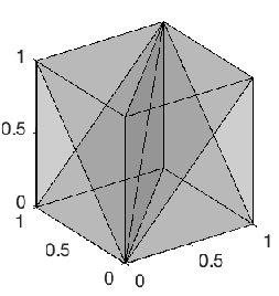
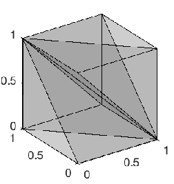
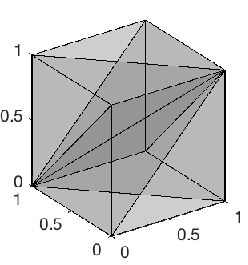
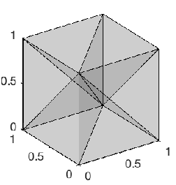
For each candidate stratification, the existing initial Monte Carlo samples are distributed to the simplices through a transformation to barycentric coordinates, and local statistics are computed. The minimum estimator variance stratification among the candidates is chosen as the initial stratification of the hypercube.
4.2 Identification of bisection planes for splitting
A stratum can theoretically be split along any one of an uncountable number of planes, but finding a nearly optimal plane may require an unnecessary amount of work, especially since we expect more information through new samples to change the shape of the optimal stratification. During stratification refinement, strata are instead split to obtain the greatest variance reduction among a finite number of possibilities. To limit the search space of possible new strata, we consider only all possible bisections into two new members of the stratum class (here: hyperrectangles or simplices) of all strata and choose the minimizer as in (14). Next we describe how this is done in the case of hyperrectangular and simplex stratifications, but note that other options such as splitting more than one stratum at once could also be implemented without major changes to the algorithm.
With a hyper-rectangular stratification, splitting must remain aligned with the coordinate system. Each time we split a stratum across dimensions, the number of strata is increased by . This is not a severe limitation on the choice of , but we do require at least one sample in each stratum, so should not be too large. With , which was also used for the numerical experiments discussed in Sect. 5, there are possible ways to split a hyperrectangle by bisection into two new hyperrectangles, as illustrated for in Fig. 3.
Simplices can be split in multiple ways to result in a refined simplex partitioning. Perhaps the simplest way to avoid excessive growth in the number of strata is to split a candidate simplex in two equal-sized simplices defined by adding the hyperplane going through the mid-point of one edge and the remaining vertices that are not the end points of the edge whose midpoint is used. As a simplex has edges, and each one corresponds to a possible bisection, there are ways to split a simplex using this method. This is illustrated for in Fig. 4, with six different ways to bisect the simplex, each producing two new simplices. Clearly, a larger number of conditional variances for each tentative bisection must be computed, compared to the case of hyperrectangular dynamic stratification. Bisection leads to very simple computation of the probability measure of new strata: they are just 1/2 of the measure of their parent stratum. A straightforward generalization of the above described bisection method is to split along a plane where the split point of the edge is not a midpoint. In that case, the volume can be computed by , where is the set of vertices.
4.3 Sequential allocation of samples
The stratification is dynamically updated by bisection (or other means of splitting) of existing strata. We refer to a cycle of bisection and subsequent sampling as an iteration of Algorithm 1. At every iteration and for a given value , samples are newly distributed and added to the current stratification for an asymptotic (i.e., for sufficiently large) sample allocation according to the rates
As the hybrid parameter is fixed, we will suppress the explicit dependence and simply write . Adding these samples at the current iteration to the current stratification then amounts to adding new samples to stratum satisfying
i.e., striving to fulfill as in (9), assuming a fixed stratification. Here denotes the smallest integer greater than or equal to . Even for hybrid sampling rules where a fraction of samples is proportionally allocated (i.e., ), some strata may not be assigned new samples in every iteration. Eventually, all strata will receive new samples, but for strata where variability has been underestimated this can require several iterations and may not happen before the total sampling budget of samples has been reached. To avoid that a stratum where the standard deviation has mistakenly been assigned to be zero does not get updated, we may reserve at least one sample for every stratum, independent of the sampling rates. Hence, we may alternatively use the allocation rule
In case at least one stratum has been oversampled, e.g., as a result of a stratum being created from a parent stratum with larger variance, both sampling rules require a total number of samples exceeding . In these cases, we add samples according to the allocation rule as long as the total sampling budget is not exceeded.
Since the stratification is dynamic and changes with (almost) every iteration, there is a trade-off between choosing large enough to approximately satisfy the rates , and small enough to save samples for further refinement of the stratification. A reasonable compromise may be to always add a constant times the current number of strata so that every stratum gets on average new samples in each iteration,
| (17) |
We emphasize that the distribution of samples is not restricted to the choice (17), and other choices may significantly impact the performance of the algorithm. At the same time, the results in Sect. 3.3 offer a convenient probabilistic interpretation of the value for in (17) as the (stratification averaged) likelihood of drastically underestimating a local stratum variance.
4.3.1 Updating stratum statistics
Updating the statistics of each stratum in every iteration may become quite costly for large sample sizes, in particular if only a small number of samples are added at every iteration so that many iterations are performed. Instead of recomputing the sample means and standard deviations from scratch using the standard formulae, we use the following update formulae
| (18) | ||||
| (19) |
which follows the ideas of Welford’s online algorithm [38]. Here, the subscripts ’old’ and ’new’ denote two independent sample sets of the same quantity. These expressions are not only used for the stratum means and standard deviations, but also to update the corresponding quantities for potential splits, i.e., possible new strata.
4.4 Setting the hybrid sampling parameter
The choice of the hybrid parameter , which controls the sampling allocation rule, is affected by two opposing trends: robustness and variance reduction. In Sect. 3.3 we have discussed that optimal allocation with can lead to poor performance of the adaptive procedure described in Algorithm 1 whenever the variances in high-variance strata are drastically underestimated. This is because the iterative procedure in Algorithm 1 with may never (e.g., in the case of zero variance estimates) add new samples to these strata so that the underestimation cannot be recovered, not even asymptotically. In that sense, the choice lacks robustness. In contrast, proportional allocation (i.e., ) is the most robust in that regard as it does not rely on estimates of the strata standard deviations; cf. also Lemma 1. On the other hand, the results in Sect. 2.3 indicate that optimal allocation with does not only offer minimal variance for a fixed stratification, but it is also optimal with respect to the size of a stratification when the function is discontinuous. This is in particular relevant for the class of functions of interest in this work. However, Lemma 3 also reveals that suitable values of smaller than may still offer quasi-optimal variance reduction for discontinuous functions. The summary of these two opposing effects is therefore that one should select as small as possible yet large enough to provide quasi-optimal variance reduction. The numerical examples presented in Sect. 5 contains both results for fixed values of , and dynamic choice of , to be described next.
4.4.1 Dynamic choice of the hybrid parameter
An alternative is to chose dynamically across iterations of the adaptive stratification algorithm described in Algorithm 1. The procedure that we describe in the following is based on the intuition that at the beginning of the iterative procedure we may have unreliable estimates of the strata standard deviations, so that small is advisable. Eventually, as the procedure adapts the stratification and increasingly more samples are being generated, one expects that more reliable estimates of the standard deviations are available for values of , so that large is desired for quasi-optimal variance reduction.
To formalize this intuition, let denote the iteration counter of Algorithm 1 and suppose that the hybrid parameter is initialized with for the first iteration (e.g., is natural). Let denote the value of the hybrid parameter used during the -th iteration. At the end of that iteration (line 21 in Algorithm 1), the value of the hybrid parameter for the iteration should then be selected in a way that provides a good compromise between variance reduction and robustness. Here we describe an update based on the stratified sampling estimators variance ; cf. Sect. 2.3. If the exact strata standard deviations were known, then the optimal variance reduction would be achieved for . However, the standard deviations are estimated based on the samples that have been generated during the iterations so far. Hence, only the empirical variance constant is available. Naively selecting the hybrid parameter for iteration as , where contains the estimated strata standard deviations using the samples available at iteration , may result in spurious effects due to the lack of robustness, as the empirical variance constant introduces an error. In fact, in view of the asymptotic distribution characterized in Lemma 2, the empirical variance constant is random, and it will fluctuate around , where those fluctuations will be asymptotically normally distributed. The size of the fluctuations can then be approximately quantified via the limit distribution’s variance, which we write as to emphasize the dependence on both the strata standard deviations and the kurtosis for practical considerations. Therefore, instead of selecting by minimizing at iteration we incorporate these fluctuations and consider the minimization of the empirical function
where the index indicates that and contain the estimated strata standard deviations and kurtosis, receptively, using the samples available at iteration . That is, for every iteration , the function corresponds to the upper end of the approximate (asymptotic) confidence interval for the variance constant . Moreover, it satisfies almost surely, since implies . One therefore expects that the update by satisfies asymptotically as . To further robustify the iterative selection of , one could, for example, choose as the smallest value in that already provides , of the optimal (i.e., minimal) upper confidence band for the variance constant. The complete selection procedure outlined above is summarized in Algorithm 2.
Notice that the choice coincides with the case of no additional robustification. Moreover, step 2 of Algorithm 2 requires estimating both and based on the available samples at iteration . To minimize the risk of drastically misestimating the strata variances (and thus the kurtosis), cf. inequality (15), we propose to use KDE-based techniques moment estimates discussed in Sect. 3.3, which introduce additional smoothing for strata with small observed variability.
5 Numerical results
As discussed in Sect. 2, for a given stratification (and if exact sample allocation rules are available) stratified sampling yields an unbiased estimator of , whose variance is reduced compared to that of a classic Monte Carlo estimator; cf. (6). In fact, the ratio of the Monte Carlo estimator’s variance and a hybrid stratified sampling estimator’s variance gives rise to as a measure of the speedup in view of the central limit theorem (3). Indeed, the speedup
| (20) |
can be seen as the factor of how many more simulations (i.e., evaluations of the model ) are needed to achieve a certain mean squared error goal when using a Monte Carlo estimator compared to a hybrid stratified sampling estimator.
The adaptive stratification procedure introduced in this work aims at minimizing the stratification estimator’s variance by consecutively refining high variance strata. That is, the procedure is designed to maximize the speedup even in the presence of heterogeneous features of . A consequence of this dynamic sampling-based adaptation is that it is no longer guaranteed that the estimator at the final iteration will be a statistically unbiased estimator of for a finite sample size , due to the dependencies on the previously sampled variables and strata refinements. However, taking advantage of the hybrid sample allocation and following the directives introduced in Sect. 3, the adaptive stratified sampling estimator is still asymptotically unbiased for any . Moreover, numerical comparisons (not shown here) of the empirical adaptive stratified sampling estimators’ bias with the empirical Monte Carlo bias for the test cases considered in the following indicated that both terms are of similar size.
Recall that in this work, we assume that the total cost of obtaining samples of the function of interest is vastly higher than the cost of the dynamic stratification and allocation of samples. In what follows, the performance of the algorithm presented in previous sections is evaluated on a range of different test cases. We note that we do not present trivial cases where e.g., a discontinuity can be exactly tessellated by the kind of stratification chosen here (hyperrectangles or simplices), but report that for such cases the speedups compared to standard Monte Carlo become arbitrarily large. A discontinuity defined by of a hypersphere is thus a nontrivial and more insightful test case where the number of stochastic dimensions can be varied to investigate how the performance depends on the dimensionality of the problem (Sect. 5.1). The variance is strictly localized to strata that contain the boundary of the hypersphere, and zero elsewhere. That is, the challenging aspect of these test cases for the adaptive stratification procedure is the identification (and adaptive isolation) of a discontinuity. Next, an idealized model for the critical pressure in a faulted reservoir based on analytical physical expressions is investigated (Sect. 5.2). The model exhibits both discontinuities and regions of sharp but continuous variation. Finally, we perform numerical tests on the Sod test case from fluid dynamics, and a vertical equilibrium porous medium model describing subsurface CO2 storage (Sects. 5.3 and 5.4). All these cases exhibit discontinuous dependence of the quantity of interest (QoI) with respect to the stochastic parameters , as is depicted in Fig. 5 and described in more details in subsequent subsections.


For all test problems, we present results using hybrid sampling with (proportional sampling), , and determined dynamically on using Algorithm 2.
5.1 Hyperspherical discontinuity in multiple dimensions
Consider the unit step function with all coordinates within the unit intervals, and restricted by the hypersphere in dimensions with center at the origin and radius chosen so that the hypersphere’s volume is equal to ,
| (21) |
An example of the development of the adaptive stratification is shown for the case in Fig. 6. Starting from 30 uniformly distributed samples in the unit square, a total of 10,000 samples are distributed adaptively, resulting in a final stratification consisting of 17 strata. The samples are progressively allocated to strata that contain the discontinuity, i.e., have non-zero variances. In addition, 10% of samples every iteration are allocated proportionally to enable detecting unseen solution features.


Speedups for are shown in Figs. 7-9, respectively. For and the largest sample sizes, the speedups are 2-3 orders of magnitude compared to standard Monte Carlo sampling. For , the corresponding speedups are 10-40, and for typically 5-10. Small values of , intuitively corresponding to more greedy yet more “risky” stratifications in view of Sect. 4.3, tend to slightly increase speedup, but the pattern is not unambiguous. Dynamically choosing in most cases resembles sampling with fixed with some notable differences for smaller sample sizes and .


5.2 Geomechanics fault surface stress problem
Consider injection through a well into a porous medium with unknown permeability and unknown location of a fault. We employ a simplified model for the surface stress at a fault assuming single-phase flow and no poro-elastic effects of injection, as in [25]. The background stress field only changes at the injection surface, and hydrostatic pressure is assumed. The QoI is the stress threshold that indicates fault stability,
where is a Coulomb fault failure criterion. The friction drop is 0.8, the shear stress is 20 MPa, the normal stress is the difference between an original stress assumed to be 50 MPa and the pressure ; where kg/m3 (density water), (gravitational constant), m (depth of caprock), m (height of injection formation), and the hydraulic head is a function of the well distance and given by Eq. (2.46) in [25]. The stochastic input parameters are the well distance (in meters) with distribution , and the friction coefficient (dimensionless) with lognormal(0.2, 0.7) distribution.
Figure 10 shows the variance ratios for the fault surface problem as a function of total number of samples, for and dynamic using hyperrectangles and simplices for the adaptive stratifications. For this problem, the best performance is achieved for hyperrectangular stratifications with proportional allocation () with speedups exceeding three orders of magnitude compared to Monte Carlo for the largest sample sizes investigated. This contrasts with the hyperspherical test cases previously presented, where simplices and nearly optimal allocation yield the best results.
5.3 Sod shock tube problem
The Sod test case describes the time-dependent behavior of two gas phases with different phase properties, separated by a membrane that is instantly removed at time 0. The problem can be modeled by the one-dimensional Euler equations and has been investigated in the uncertainty quantification literature to illustrate challenges related to discontinuities in stochastic space [29, 36, 28]. We assume the following three uncertain parameters: left state density , right state density , and initial location of the membrane with distribution . The quantity of interest is the density at .
The speedups for hyperrectangles and simplices, hybrid sampling with , , and dynamic , are shown in Fig. 11. The best performance is obtained with hyperrectangular stratification, despite a curved hypersurface discontinuity, see Fig. 5(b).
5.4 Vertical equilibrium model of CO2 storage
Subsurface permanent CO2 storage involves injection of large quantities of CO2 into porous reservoirs with largely unknown physical properties. The varying temporal and physical scales calls for simplified-physics models, achieved, e.g., by vertical equilibrium assumptions and dimension reduction by integration over the vertical direction [25]. The result is a nonlinear hyperbolic conservation law with discontinuous flux function, where the solution represents the saturation of CO2 as a function of space and time. For reproducibility, Table 1 contains all values relevant for the setup of the problem, including distributions for four random parameters: permeability, brine mobility, CO2 mobility, and background flow rate. A more detailed description of the problem, including the conservation law and its time-dependent solution, can be found in [22, 27]. Although not explicitly referred to in this paper, Table 1 lists notation for various parameters consistent with [27], also to facilitate reproducibility.
| Parameter | Notation | Value/Distribution |
|---|---|---|
| Porosity | 0.15 | |
| Residual brine saturation | 0.1 | |
| Residual CO2 saturation | 0.1 | |
| Slope angle | 0.005 | |
| Injection time | 20 years | |
| Injection rate | m/s | |
| CO2 mobility | Uniform ms/kg | |
| Brine mobility | Uniform ms/kg | |
| Background flow | Exponential, mean m/s | |
| Permeability | Lognormal, mean 200 mD, std 50 mD |
The QoI is the height of the CO2 plume 100 m downstream of the injection location, 600 years after the end of injection. Speedups for the CO2 problem as a function of the total number of samples are shown in Fig. 12. Speedup is observed for all sampling schemes, even for the smallest sizes of sample sets. This problem exhibits zero or small variability away from the discontinuities, as indicated in Fig. 5(c), making it a particularly suitable candidate for the proposed method. At the same time, the number of dimensions ( due to being a function of the ratio of the phase mobilities, rather than their individual values) already requires a large number of samples to give speedups greater than an order of magnitude.
6 Conclusions
We have introduced a novel stratified sampling method with adaptive stratification and sequential, hybridized allocation of samples. For a fixed stratification, the sample allocation asymptotically approaches a prescribed linear combination of proportional and optimal allocation. Letting a fraction of samples be allocated proportionally adds robustness to the adaptive method, as the stratum standard deviations are not a priori known but estimated on-the-fly as samples are added. Moreover, a greedy approach is used to split the stratum that results in the largest reduction of the stratified sampling estimator’s current variance. Kurtosis dependent estimates are provided that allow to quantify the probability of drastically underestimating local strata variances and, thus, of failing to identify strata that should be refined.
To maintain prescribed stratum sampling rates and for ease of implementation, a new stratum that arises after re-stratification should be contained within a single parent stratum, and it should retain the same geometrical shape. In this work, we suggest using hyperrectangles or simplices for the stratification, as either of these shapes can be bisected and the result is two new hyperrectangles or simplices. In fact, both classes of tessellations allow for a flexible partition of the stochastic domain.
The proposed method is anticipated to result in significant speedups for problems where the variability is localized in random space, e.g., the PDE solutions describing physical problems with uncertain parameters and exhibiting steep gradients or discontinuities. In contrast to, e.g., localized response surface methods based on function approximations, an advantage of the proposed method is that accurate identification of steep features is not necessary to obtain good results. Confining sharp features to strata of small measure is often sufficient to vastly outperform standard Monte Carlo sampling. This has been verified experimentally through various test cases, exhibiting speedups of up to three orders of magnitude compared to standard Monte Carlo.
Acknowledgements
The authors would like to thank Eirik Keilegavlen at the University of Bergen for the setup of the fault surface stress problem. The first author was funded by the Research Council of Norway through the project Quantification of fault-related leakage risk (FRISK) under project number 294719. A CC BY or equivalent licence is applied to the author accepted manuscript arising from this submission, in accordance with the grant’s open access conditions.
Appendix A Derivation of the gradient of the variance constant
Introduce the functions
for any . Then
so that . To quantify the robustness of the variance reduction with respect to perturbation in , we compute the gradient of . Therefore, we first compute the partial derivative of with respect to the component of as
where denotes the Kronecker delta: if and else. Next we compute the component of the gradient of with respect to , which, after some algebra, can be written as:
Finally, using the fact that
we can eventually write the partial derivative of as
Appendix B Further motivation for splitting adaptively
B.1 Variance reduction by splitting
Consider an arbitrary stratum with a partition defining a refined stratification. We are interested in the effect of splitting on the variance of the estimator. Without loss of generality, assume that (we may always subtract a constant without changing the variance), and let the relative measure of and be and (the measure of itself does not matter). Then,
| (22) |
where the second equality follows from and being disjoint and the relation
The right-hand side of Eq. (22) equals the variance contribution to the estimator from the two newly created strata. Thus, we have shown that splitting of a stratum always reduces the variance of the estimator. that optimal allocation is maintained after splitting.
B.2 Stratification of domains of discontinuous functions
Let and be two subdomains that forms a partition of , separated by a hypersurface . Let be a piecewise constant function on , defined by
| (23) |
where and are constants, and consider a neighborhood around . Denote the measure of and by and , respectively, and and . Setting we have
| (24) |
where we have used that , and . Note that (24) is similar to the expression for the global variance,
To minimize the variance, we see from (24) that the stratum should be small, whereas the local variances in and are identically zero (since is constant).
References
- [1] S. Asmussen and P. W. Glynn. Stochastic simulation: algorithms and analysis, volume 57. Springer, New York, 2007.
- [2] L. Cabral Pereira, M. Sánchez, and L. J. do Nascimento Guimarães. Uncertainty quantification for reservoir geomechanics. Geomech. Energy Envir., 8:76–84, 2016. Themed Issue on Selected Papers Symposium of Energy Geotechnics 2015 — Part II.
- [3] M. Christie, V. Demyanov, and D. Erbas. Uncertainty quantification for porous media flows. J. Comput. Phys., 217(1):143–158, 2006.
- [4] K. A. Cliffe, M. B. Giles, R. Scheichl, and A. L. Teckentrup. Multilevel Monte Carlo methods and applications to elliptic PDEs with random coefficients. Comput. Visual Sci., 14(1):3–15, 2011.
- [5] W. G. Cochran. Sampling Techniques. John Wiley & Sons, New York, 3rd edition, 1977.
- [6] François Cuvelier and Gilles Scarella. Vectorized algorithms for regular tessellations of d-orthotopes and their faces. working paper or preprint, November 2017.
- [7] A. DasGupta. Asymptotic theory of statistics and probability. Springer, New York, 2008.
- [8] C. De Luigi and S. Maire. Adaptive integration and approximation over hyper-rectangular regions with applications to basket options pricing. Monte Carlo Methods Appl., 16:265–282, 12 2010.
- [9] J. Dick, F. Y. Kuo, and I. H. Sloan. High-dimensional integration: The quasi-Monte Carlo way. Acta Numerica, 22:133–288, 2013.
- [10] P. Étoré, G. Fort, B. Jourdain, and E. Moulines. On adaptive stratification. Ann. Oper. Res., 89(1):127–154, 2011.
- [11] P. Étoré and B. Jourdain. Adaptive optimal allocation in stratified sampling methods. Methodol. Comput. Appl., 12(3):335–360, 2010.
- [12] M. B. Giles. Multilevel Monte Carlo methods. Acta Numer., 24:259–328, 2015.
- [13] M. B. Giles and A.-L. Haji-Ali. Multilevel nested simulation for efficient risk estimation. SIAM/ASA J. Uncertain. Quantif., 7(2):497–525, 2019.
- [14] A. Gorodetsky and Y. Marzouk. Efficient localization of discontinuities in complex computational simulations. SIAM J. Sci. Comput., 36(6):A2584–A2610, 2014.
- [15] A.-L. Haji-Ali, F. Nobile, and R. Tempone. Multi Index Monte Carlo: when sparsity meets sampling. Numer. Math., 132(4):767–806, 2016.
- [16] S. Hosder, R. Walters, and M. Balch. Efficient uncertainty quantification applied to the aeroelastic analysis of a transonic wing. In 46th AIAA Aerospace Sciences Meeting and Exhibit, 2008.
- [17] J. D. Jakeman, A. Narayan, and D. Xiu. Minimal multi-element stochastic collocation for uncertainty quantification of discontinuous functions. J. Comput. Phys., 242:790– 808, 2013.
- [18] D. P. Kroese, T. Taimre, and Z. I. Botev. Handbook of Monte Carlo methods. Wiley New Jersey, 2011.
- [19] S. Krumscheid and F. Nobile. Multilevel Monte Carlo Approximation of Functions. SIAM/ASA J. Uncertain. Quantif., 6(3):1256–1293, 2018.
- [20] S. Krumscheid, F. Nobile, and M. Pisaroni. Quantifying uncertain system outputs via the multilevel Monte Carlo method—Part I: Central moment estimation. J. Comput. Phys., 414, 2020.
- [21] H. W. Kuhn. Some combinatorial lemmas in topology. IBM J. Res. Dev., 4(5):518–524, November 1960.
- [22] C. W. MacMinn, M. L. Szulczewski, and R. Juanes. CO2 migration in saline aquifers. part 1. capillary trapping under slope and groundwater flow. J. Fluid Mech., 662:329–351, 2010.
- [23] F. Müller, P. Jenny, and D. W. Meyer. Multilevel Monte Carlo for two phase flow and Buckley-Leverett transport in random heterogeneous porous media. J. Comput. Phys., 250:685–702, 2013.
- [24] H. Niederreiter. Random number generation and quasi-Monte Carlo methods. Society for Industrial and Applied Mathematics (SIAM), Philadelphia, PA, 1992.
- [25] J.M. Nordbotten and M.A. Celia. Geological Storage of CO2: Modeling Approaches for Large-Scale Simulation. Wiley, 2011.
- [26] T. N. Palmer. Predicting uncertainty in forecasts of weather and climate. Rep. Prog. Phys., 63(2):71–116, 2000.
- [27] P. Pettersson. Stochastic Galerkin formulations for CO2 transport in aquifers: Numerical solutions with uncertain material properties. Transport Porous Med., 114(2):457–483, 2016.
- [28] P. Pettersson, G. Iaccarino, and J. Nordström. A stochastic Galerkin method for the Euler equations with Roe variable transformation. J. Comput. Phys., 257:481–500, 2014.
- [29] G. Poëtte, B. Després, and D. Lucor. Uncertainty quantification for systems of conservation laws. J. Comput. Phys., 228(7):2443–2467, 2009.
- [30] W. H. Press and G. R. Farrar. Recursive stratified sampling for multidimensional Monte Carlo integration. Comput. Phys., 4(2):190–195, 1990.
- [31] A. Rushdi, L. P. Swiler, E. T. Phipps, M. D’Elia, and M. S. Ebeida. Vps: Voronoi piecewise surrogate models for high-dimensional data fitting. Int. J. Uncertain. Quan., 7(1):1–21, 2017.
- [32] R. J. Serfling. Approximation theorems of mathematical statistics. John Wiley & Sons, Inc., New York, 1980.
- [33] M. D. Shields. Refined latinized stratified sampling: A robust sequential sample size extension methodology for high-dimensional latin hypercube and stratified designs. Int. J. Uncertain. Quan., 6(1):79–97, 2016.
- [34] M. D. Shields, K. Teferra, A. Hapij, and R. P. Daddazio. Refined stratified sampling for efficient Monte Carlo based uncertainty quantification. Reliab. Eng. Syst. Safe., 142:310–325, 2015.
- [35] D. M. Tartakovsky and S. Broyda. PDF equations for advective-reactive transport in heterogeneous porous media with uncertain properties. J. Contam. Hydrol., 120-121:129–140, 2011.
- [36] J. Tryoen, O. Le Maître, M. Ndjinga, and A. Ern. Intrusive Galerkin methods with upwinding for uncertain nonlinear hyperbolic systems. J. Comput. Phys., 229(18):6485–6511, 2010.
- [37] R. Vershynin. High-dimensional probability, volume 47 of Cambridge Series in Statistical and Probabilistic Mathematics. Cambridge University Press, Cambridge, 2018. An introduction with applications in data science.
- [38] B. P. Welford. Note on a method for calculating corrected sums of squares and products. Technometrics, 4:419–420, 1962.
- [39] J. A. S. Witteveen and G. Iaccarino. Simplex stochastic collocation with random sampling and extrapolation for nonhypercube probability spaces. SIAM J. Sci. Comput., 34(2):A814–A838, 2012.
- [40] D. Xiu. Numerical methods for stochastic computations: A spectral method approach. Princeton University Press, Princeton, NJ, 2010.