Confronting the inverse seesaw mechanism with the recent muon g-2 result
Abstract
Since the heavy neutrinos of the inverse seesaw mechanism mix largely with the standard ones, the charged currents formed with them and the muons have the potential of generating robust and positive contribution to the anomalous magnetic moment of the muon. However, bounds from the non-unitary in the leptonic mixing matrix may restrict so severely the parameters of the mechanism that, depending on the framework under which the mechanism is implemented, may render it unable to explain the recent muon g-2 result. In this paper we show that this happens when we implement the mechanism into the standard model and into two versions of the 3-3-1 models.
I Introduction
The recent measurement of by the E989 experiment at Fermilab Abi et al. 2021, in agreement with the previous BNL E821 result Bennett et al. 2006, yields a discrepancy from the standard model (SM)
It represents a hint of physics beyond standard model (BSM) Keshavarzi et al. 2021. The easiest way to generate new contributions to the g-2 of the muon is by means of new interactions involving the leptonic sector (See Ref.Lindner et al. 2018 for an extended review). Furthermore, the SM cannot address neutrino masses. Therefore, it is appealing to investigate models that can accommodate both problems.
There are several ways to explain neutrino masses, but in this work, we will focus on the inverse seesaw (ISS) mechanismMohapatra and Valle 1986; Mohapatra 1986; Dias et al. 2011. It is a genuine TeV scale seesaw mechanism whose signature, heavy neutrinos ’s, is supposed to manifest at TeV scale. This interesting aspect allows us to confront the mechanism with existing TeV scale probes. In light of the recent measurement conducted by the Fermilab g-2 experiment, one might wonder whether one can successfully explain g-2 with the ISS.
The minimum SM extension capable of embedding the ISS has been addressed previously to analyze the corresponding g-2 contributions for sterile fermion states Abada et al. 2014. We consider the contributions for the g-2 of the muon due exclusively to the heavy neutrinos of the ISS mechanism. To do this, we consider models that do not accommodate the recent muon g-2 result (SM and some versions of the 3-3-1 model) and implement the ISS mechanism in them economically, where only the new neutral fermion singlets are added to the models in question. We then try to obtain a region of parameter space that could accommodate the recent measurement of g-2 of the muon and agree with some bound over the mechanism.
Our work is organized in the following way: In Sec. II, we present the main ingredients of the mechanism and develop our approach. In Sec. III, we implement the mechanism into the standard model, the minimal 3-3-1 model and the 3-3-1 model with right-handed neutrinos and explicit the terms that give the main contributions to the g-2 of the muon due to the heavy neutrinos. In sec. IV, we present our numerical results. We finalize presenting our conclusions in Sec. V.
II The main ingredients of the mechanism
II.1 Framework and nonunitarity costraint
The mechanism involves nine neutral fermions with specific chirality , and composing the following mass terms
| (1) |
where , and are generic mass matrices. We rearrange things so that in the basis we may write
| (2) |
where,
| (3) |
In recognizing,
| (4) |
we write
| (5) |
This mass matrix may be diagonalized by a mixing matrix given bySchechter and Valle 1982; Hettmansperger et al. 2011
| (6) |
such that
| (7) |
where we have . In terms of the original parameters, we have,
| (8) |
Observe that the diagonalization of must lead to the eigenvalues , which we assume are associated with the following eigenvectors .
Now comes the essence of the mechanism. For belonging to the electroweak and to the TeV scale, we just need that lepton number be explicitly violated at sub-keV scale (keV) in order to have at sub-eV scale. Of course, we are assuming that are the standard neutrinos.
Concerning the heavy neutrinos, we assume that is diagonalized by , and that the eigenvectors are given by , with , whose masses lie around . Moreover, the mixing among the neutrinos allows us to write the standard flavor neutrinos as the following combinations of the physical neutrinosDev and Mohapatra 2010
| (9) |
where . In view of the structure of this mixing, all deviation from unitarity is determined by the Hermitian matrix,
| (10) |
We point out that it does not depend on the parametrization of the PMNS matrix. This matrix is known as the nonunitarity parameter and have a crucial role in this paper. Current bounds on nonunitarity effects gives Fernandez-Martinez et al. 2016
| (11) |
II.2 Our approach
In the usual approach, the matrices and are considered as diagonal ones. In this case determines the texture of .
We take a different approach now. We assume that and are diagonal and degenerated: and . Then Eq. (8) get
| (12) |
which leaves responsible for the texture of . It happens that in our approach the parameter , defined in Eq. (10), takes the form
| (13) |
which, according to the bound in Eq. (11), yields,
| (14) |
This is nice because the nonunitarity constraint is favoring below keV scale to yield standard neutrino masses at eV scale.
After diagonalizing above, we obtain
| (15) |
where . Inverting these matrices, we get,
Once we know the absolute values of and having from the experiments, we obtain the texture of .
Now we focus on the pattern of . For this we diagonalize given in Eq. (4) which in our approach:
| (16) |
For the eigenvalues of are,
| (17) |
which means that the six heavy neutrinos are practically mass degenerate with the values lying around . In this case, the mixing matrix, , that diagonalizes develops the following approximated pattern
| (18) |
In summary, in our approach, is responsible for the texture of the standard neutrino mass matrix, while the assumption infers the pattern of . This method eases the assessment of the heavy neutrinos contributions to g-2 significantly consistently. With this method at hand, we can solidly investigate if the inverse seesaw mechanism may explain g-2 Abi et al. 2021.
We remind the reader that we will adopt throughout the most recent result from the Muon g-2 Experiment at Fermilab, which combined with previous Brookhaven National Laboratory E821 measurement reported . The difference has a significance of Abi et al. 2021; Keshavarzi et al. 2021. See Ref. Lindner et al. 2018 for an extensive explanation about how the anomaly can be weakened or strengthened.
The implementation of the ISS requires the introduction of new neutral fermions, , to the original fermion content of the model in question. In extended gauge theories that feature the presence of new vector gauge bosons, such neutral fermions will appear in the charged currents involving exotic charged gauge bosons represented by . In a general way, we write down these interactions through the following terms
| (19) |
After some steps, the contribution of these new interactions to the g-2 of the muon is given byLindner et al. 2018,
| (20) |
where
| (21) |
and , .
We apply this method to obtain the contribution to the g-2 stemming exclusively from the new ingredients of the ISS mechanism when implemented in models from starters that do not accommodate g-2.
III ISS contributions to the g-2 of the muon
III.1 Standard model
To implement the ISS mechanism in a minimal way into the standard model, we need to add six new neutral fermions as singlets field, so the leptonic content becomes,
where . The scalar sector is assumed to be composed uniquely by the standard Higgs
With these new fields we can form the following new terms in addition to all standard ones,
| (24) |
where and . When of the spontaneous breaking of the symmetry, where , we obtain the following mass terms,
| (25) |
where and .
Observe that Eq. (25) recovers Eq. (1) which means that we have the ISS mechanism. Thus, all the step done above is valid here.
Through mixing, Eq. (9), the ISS mechanism gives rise to the following Lagrangian,
| (26) |
where are heavy pseudo-Dirac neutrinos. Notice that the product can be approximated by,
| (27) |
It is clear that the six new pseudo-Dirac neutrinos contribute to g-2. Then, from Eq. (26) and Eq. (19) we can easily identify , and that appear in Eq. (20). We also set and . After all these considerations, we are ready to calculate the contribution from Pseudo-Dirac ’s to g-2 due to the interactions in Eq. (26).
III.2 Minimal 3-3-1 model
This model is based on the (3-3-1) gauge groupPisano and Pleitez 1992; Frampton 1992. In it, all leptons of each family compose a triplet in the following way,
where . Through this feature, we can understand the quantization pattern of electric charges de Sousa Pires and Ravinez 1998. Moreover, the gauge anomalies are canceled only when three families are considered at once Foot et al. 1993. There are several additional interesting aspects Dias et al. 2003; Pal 1995; Dias et al. 2004; Alves et al. 2011; Alves et al. 2013. The gauge sector of the model features the standard gauge bosons and five other ones as a new , two new single charged gauge bosons and two doubly charged gauge bosons . Their respective neutral and charged currents are found in Cao and Zhang 2016. It has been shown in de Jesus et al. 2020 that all these interactions are not enough to accommodate the recent muon g-2 result. Hence, it brings up whether the ISS mechanism can foot the bill while successfully generating small masses.
For the implementation of the mechanism, we add the six neutral fermions and, as discussed previously. The minimal set of scalars necessary to break spontaneously the symmetry and generate masses for all massive particles, except neutrinos, are three triplets , , and a sextet of scalar . With this we form the terms
| (31) |
When develop vev, , we have the following mass terms,
| (32) |
where . These mass terms recover the characteristic mass matrix of the ISS mechanism given in Eq. (3). Then all approach developed in Sec. II is applicable here.
In what concern the contributions to the g-2 of the muon due to the heavy neutrinos ’s, they arise from the interactions of these neutrinos with the charged gauge bosons and ,
| (33) | |||||
, and are exactly those in Sec. II. Our task here is to check if this new interactions give significant contributions to the g-2 of the muon.
III.3 3-3-1 model with right-handed neutrinos
In this version of the 3-3-1 modelsMontero et al. 1993; Singer et al. 1980; Foot et al. 1994 the third component of the leptonic triplet is occupied by the right-handed neutrinos invoked by the ISS mechanismDias et al. 2012
| (34) |
This version shares the same main features that the minimal one in respect to anomaly cancellation, electric charged quantization and strong-CP problem with the additional one of having natural dark matter candidatesde S Pires and da Silva 2007; Mizukoshi et al. 2011; Dutra et al. 2021. However, it is a new model with its gauge sector being composed by the standard gauge bosons and five other ones as a new , two new single charged gauge bosons and two neutral, but non-hermitian, gauge bosons . The interactions of these gauge bosons with the neutral and charged currents is found in Long 1996. It was checked in de Jesus et al. 2020 that all these interactions are not enough to accommodate the recent muon g-2 result, and again this provides a strong motivation for we check if the implementation of the ISS mechanism would give significant contributions to the g-2 of the muon.
For the implementation of the mechanism, we just need to add three new neutral fermions in the singlet form, . In this model the minimal set of scalars necessary to break spontaneously the symmetry and generate masses for all massive particles, except neutrinos, are three triplets of scalars , , . With this minimal particle content we form the following terms that will trigger the ISS mechanism
| (35) |
When and develop their vev’s, and , we have the following mass terms,
| (36) |
where and . These mass terms recover the characteristic mass matrix of the ISS mechanism given in Eq. (3). Then all approach developed in Sec. II is applicable here with specific care because, now, is an antisymmetric matrix and, due to this, we can not take it diagonal. But it is possible to take it degenerated. In this case we have
| (37) |
Following this, taking , we have for the nonunitary parameter, defined in Eq. (10)
| (38) |
In what concern the contributions to the g-2 of the muon due to the heavy neutrinos ’s, they arise from the interactions of these neutrinos with the charged gauge bosons and ,
| (39) | |||||
with
| (40) |
Observe that all the new contributions to g-2 of the muon, in all three cases, are due to interactions involving charge currents and single charged gauge bosons as represented in Fig. 1 for being the standard gauge boson or . For previous works addressing g-2 into this model, see Refs. Hue et al. 2020; Hue et al. 2021

We are now ready to calculate such contributions in all three cases. We do this and present our numerical results in the next section.
IV Numerical results
For our numerical calculations, we made use of the code Queiroz 2021, developed in de Jesus et al. 2020. Then, after configuring this algorithm for each case, we solved numerically the integral in Eq. (20).
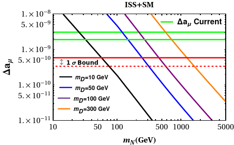
Our first result is presented in Figs. 2 and 3, where we consider the case of the ISS mechanism implemented into the Standard Model (ISS + SM). Notice that the new interactions in Eq. (26) involving heavy neutrinos explain the recent muon g-2 results for varying from few tens up to thousands of GeV’s. However, the current bound on the nonunitarity parameter , Eq. (13), requires the model to live in a different corner of the parameter space, delimited by the blue region. Thus, the regions do not overlap, and we conclude that one cannot simultaneously explain g-2 and be consistent with nonunitarity. This means that the ISS mechanism, on its own, is not able to explain the muon g-2 result, at least when implemented in the standard model.
In Figs. 4 and 5 we present our results for the case of the ISS mechanism implemented into the minimal 3-3-1 model. For minimal 3-3-1 model and for the 3-3-1 with right-handed neutrinos, we calculate the total contribution of for fixed gauge boson masses. These masses are set to be sufficiently high to avoid collider bounds, namely TeV and TeV de Jesus et al. 2020 . We see, in the left-panel, that the minimal 3-3-1 model definitely cannot explain the g-2 result. This happens mostly because the doubly-charged contribution to is dominant and negative. However, after extending the minimal 3-3-1 to accommodate the ISS, we observe new contributions for the muon g-2 in the same manner as the previous case. These new contributions are due to heavy neutrinos with interactions given in Eq. (39) and displayed in Fig. 1 with being due to the charged gauge bosons and . We present in Fig 4 our results in the plane . It is already clear that the nonunitarity constraint prevents the ISS to explain g-2. We plot our result in a different plane in Fig 5 to clearly show that these datasets are mutually exclusive. We display the favored region delimited by green lines and the with a purple line towards the bottom of the figure. Note that the nonunitarity bound lies orders of magnitude below the favored region for g-2. In summary, ISS is not the solution to g-2.
Finally, we show in Figs. 6 and 7 our results for the case of the ISS implemented into the 3-3-1 model with right-handed neutrinos. Looking at the numerical results, we arrive at the same conclusion. The ISS mechanism cannot address g-2 even in the scope of a 3-3-1 model with right-handed neutrinos.


V Discussion
We would like to emphasize that our conclusion concerning the inverse seesaw is applicable to the minimal version of the inverse seesaw, in other words, when it is implemented in the standard model, and to the 3-3-1 models studies. Our conclusion is not valid to all possible implementations of the inverse seesaw as one can always add fields in a way to change the contribution to the g-2 or circumvent the non-unitarity bounds, and consequently find different results. Obviously, such constructions are necessarily more complex. A concrete example can be found in Khalil and Un 2016; Cao et al. 2020; Cao et al. 2021.
VI Conclusions
We revisited the inverse seesaw mechanism and assessed the possibility to explain g-2 when nonunitarity constraints are considered. Firstly, we added the necessary fields to the Standard Model spectrum to realize inverse seesaw mechanism. Later, we implemented the inverse seesaw in the minimal 3-3-1 model, and in the 3-3-1 model with right-handed neutrinos. We studied the impact of the new neutral singlet fields on the lagrangians relevant for g-2 and nonunitarity studies. In all three cases, we conclusively showed that the ISS mechanism cannot address g-2 due to the stringent nonunitarity constraint that forces the masses of the particles to be orders of magnitude higher than the one required to explain g-2. This conclusion is clear in Fig. 6. In summary, our findings show that the nonunitarity constraint is severe enough to avoid the inverse seesaw mechanism to explain the recent muon g-2 result within these frameworks.
VII Acknowledgments
J.P.P has received funding/support from the European Union’s Horizon 2020 research and innovation programme under the Marie Skłodowska-Curie grant agreement No 860881-HIDDeN. C.A.S.P was supported by the CNPq research grants No. 304423/2017-3. Y.S.V acknowledges the financial support from CAPES under Grant No. 88882.375870/2019-01. FSQ is supported by the São Paulo Research Foundation (FAPESP) through grant 2015/158971, ICTP-SAIFR FAPESP grant 2016/01343-7, CNPq grants 303817/2018-6 and 421952/2018 – 0, and the Serrapilheira Institute (grant number Serra - 1912 – 31613). We dedicate this work to the memory of Joel Batista da Fonseca Neto, a great professor from UFPB who passed away recently. This work was supported by a grant from the Simons Foundation Award Number 884966, AF.
References
- Abi et al. (2021) B. Abi et al. Measurement of the Positive Muon Anomalous Magnetic Moment to 0.46 ppm. Phys. Rev. Lett., 126(14):141801, 2021. doi: 10.1103/PhysRevLett.126.141801.
- Bennett et al. (2006) G. W. Bennett et al. Final Report of the Muon E821 Anomalous Magnetic Moment Measurement at BNL. Phys. Rev. D, 73:072003, 2006. doi: 10.1103/PhysRevD.73.072003.
- Keshavarzi et al. (2021) Alex Keshavarzi, Kim Siang Khaw, and Tamaki Yoshioka. Muon : current status. 6 2021.
- Lindner et al. (2018) Manfred Lindner, Moritz Platscher, and Farinaldo S. Queiroz. A Call for New Physics : The Muon Anomalous Magnetic Moment and Lepton Flavor Violation. Phys. Rept., 731:1–82, 2018. doi: 10.1016/j.physrep.2017.12.001.
- Mohapatra and Valle (1986) R. N. Mohapatra and J. W. F. Valle. Neutrino Mass and Baryon Number Nonconservation in Superstring Models. Phys. Rev. D, 34:1642, 1986. doi: 10.1103/PhysRevD.34.1642.
- Mohapatra (1986) R. N. Mohapatra. Mechanism for Understanding Small Neutrino Mass in Superstring Theories. Phys. Rev. Lett., 56:561–563, 1986. doi: 10.1103/PhysRevLett.56.561.
- Dias et al. (2011) A. G. Dias, C. A. de S. Pires, and P. S. Rodrigues da Silva. How the Inverse See-Saw Mechanism Can Reveal Itself Natural, Canonical and Independent of the Right-Handed Neutrino Mass. Phys. Rev. D, 84:053011, 2011. doi: 10.1103/PhysRevD.84.053011.
- Abada et al. (2014) A Abada, V De Romeri, and AM Teixeira. Effect of steriles states on lepton magnetic moments and neutrinoless double beta decay. Journal of High Energy Physics, 2014(9):1–27, 2014.
- Schechter and Valle (1982) J. Schechter and J. W. F. Valle. Neutrino Decay and Spontaneous Violation of Lepton Number. Phys. Rev. D, 25:774, 1982. doi: 10.1103/PhysRevD.25.774.
- Hettmansperger et al. (2011) Hans Hettmansperger, Manfred Lindner, and Werner Rodejohann. Phenomenological Consequences of sub-leading Terms in See-Saw Formulas. JHEP, 04:123, 2011. doi: 10.1007/JHEP04(2011)123.
- Dev and Mohapatra (2010) P. S. Bhupal Dev and R. N. Mohapatra. TeV Scale Inverse Seesaw in SO(10) and Leptonic Non-Unitarity Effects. Phys. Rev. D, 81:013001, 2010. doi: 10.1103/PhysRevD.81.013001.
- Fernandez-Martinez et al. (2016) Enrique Fernandez-Martinez, Josu Hernandez-Garcia, and Jacobo Lopez-Pavon. Global constraints on heavy neutrino mixing. JHEP, 08:033, 2016. doi: 10.1007/JHEP08(2016)033.
- Pisano and Pleitez (1992) F. Pisano and V. Pleitez. An SU(3) x U(1) model for electroweak interactions. Phys. Rev. D, 46:410–417, 1992. doi: 10.1103/PhysRevD.46.410.
- Frampton (1992) P. H. Frampton. Chiral dilepton model and the flavor question. Phys. Rev. Lett., 69:2889–2891, 1992. doi: 10.1103/PhysRevLett.69.2889.
- de Sousa Pires and Ravinez (1998) Carlos Antonio de Sousa Pires and O. P. Ravinez. Charge quantization in a chiral bilepton gauge model. Phys. Rev. D, 58:035008, 1998. doi: 10.1103/PhysRevD.58.035008.
- Foot et al. (1993) Robert Foot, Oscar F. Hernandez, F. Pisano, and V. Pleitez. Lepton masses in an SU(3)-L x U(1)-N gauge model. Phys. Rev. D, 47:4158–4161, 1993. doi: 10.1103/PhysRevD.47.4158.
- Dias et al. (2003) Alex G. Dias, C. A. de S. Pires, and P. S. Rodrigues da Silva. Discrete symmetries, invisible axion and lepton number symmetry in an economic 3 3 1 model. Phys. Rev. D, 68:115009, 2003. doi: 10.1103/PhysRevD.68.115009.
- Pal (1995) Palash B. Pal. The Strong CP question in SU(3)(C) x SU(3)(L) x U(1)(N) models. Phys. Rev. D, 52:1659–1662, 1995. doi: 10.1103/PhysRevD.52.1659.
- Dias et al. (2004) Alex G. Dias, V. Pleitez, and M. D. Tonasse. Naturally light invisible axion and local Z(13) x Z(3) symmetries. Phys. Rev. D, 69:015007, 2004. doi: 10.1103/PhysRevD.69.015007.
- Alves et al. (2011) A. Alves, E. Ramirez Barreto, A. G. Dias, C. A. de S. Pires, F. S. Queiroz, and P. S. Rodrigues da Silva. Probing 3-3-1 Models in Diphoton Higgs Boson Decay. Phys. Rev., D84:115004, 2011. doi: 10.1103/PhysRevD.84.115004.
- Alves et al. (2013) Alexandre Alves, E. Ramirez Barreto, A. G. Dias, C. A. de S. Pires, Farinaldo S. Queiroz, and P. S. Rodrigues da Silva. Explaining the Higgs Decays at the LHC with an Extended Electroweak Model. Eur. Phys. J., C73(2):2288, 2013. doi: 10.1140/epjc/s10052-013-2288-y.
- Cao and Zhang (2016) Qing-Hong Cao and Dong-Ming Zhang. Collider Phenomenology of the 3-3-1 Model. 11 2016.
- de Jesus et al. (2020) Álvaro S. de Jesus, Sergey Kovalenko, Carlos A. de S. Pires, Farinaldo S. Queiroz, and Yoxara S. Villamizar. Dead or alive? Implications of the muon anomalous magnetic moment for 3-3-1 models. Phys. Lett. B, 809:135689, 2020. doi: 10.1016/j.physletb.2020.135689.
- Montero et al. (1993) J. C. Montero, F. Pisano, and V. Pleitez. Neutral currents and glashow-iliopoulos-maiani mechanism in models for electroweak interactions. Phys. Rev. D, 47:2918–2929, Apr 1993. doi: 10.1103/PhysRevD.47.2918. URL https://link.aps.org/doi/10.1103/PhysRevD.47.2918.
- Singer et al. (1980) M. Singer, J. W. F. Valle, and J. Schechter. Canonical neutral-current predictions from the weak-electromagnetic gauge group su(3) × u(1). Phys. Rev. D, 22:738–743, Aug 1980. doi: 10.1103/PhysRevD.22.738. URL https://link.aps.org/doi/10.1103/PhysRevD.22.738.
- Foot et al. (1994) Robert Foot, Hoang Ngoc Long, and Tuan A. Tran. and gauge models with right-handed neutrinos. Phys. Rev. D, 50:R34–R38, Jul 1994. doi: 10.1103/PhysRevD.50.R34. URL https://link.aps.org/doi/10.1103/PhysRevD.50.R34.
- Dias et al. (2012) A. G. Dias, C. A. de S. Pires, P. S. Rodrigues da Silva, and A. Sampieri. Simple realization of the inverse seesaw mechanism. Phys. Rev. D, 86:035007, Aug 2012. doi: 10.1103/PhysRevD.86.035007. URL https://link.aps.org/doi/10.1103/PhysRevD.86.035007.
- de S Pires and da Silva (2007) C A de S Pires and P S Rodrigues da Silva. Scalar bilepton dark matter. Journal of Cosmology and Astroparticle Physics, 2007(12):012–012, dec 2007. doi: 10.1088/1475-7516/2007/12/012. URL https://doi.org/10.1088/1475-7516/2007/12/012.
- Mizukoshi et al. (2011) J. K. Mizukoshi, C. A. de S. Pires, F. S. Queiroz, and P. S. Rodrigues da Silva. Wimps in a 3-3-1 model with heavy sterile neutrinos. Phys. Rev. D, 83:065024, Mar 2011. doi: 10.1103/PhysRevD.83.065024. URL https://link.aps.org/doi/10.1103/PhysRevD.83.065024.
- Dutra et al. (2021) Maíra Dutra, Vinícius Oliveira, C. A. de S. Pires, and Farinaldo S. Queiroz. A model for mixed warm and hot right-handed neutrino dark matter. 4 2021.
- Long (1996) Hoang Ngoc Long. Su(3su(3u(1 model with right-handed neutrinos. Phys. Rev. D, 53:437–445, Jan 1996. doi: 10.1103/PhysRevD.53.437. URL https://link.aps.org/doi/10.1103/PhysRevD.53.437.
- Hue et al. (2020) Le Tho Hue, Phong Nguyen Thanh, and Tran Dinh Tham. Anomalous Magnetic Dipole Moment in 3-3-1 Model with Inverse Seesaw Neutrinos. Commun. in Phys., 30(3):221–230, 2020. doi: 10.15625/0868-3166/30/3/14963.
- Hue et al. (2021) L. T. Hue, H. T. Hung, N. T. Tham, H. N. Long, and T. Phong Nguyen. Large and signals of decays in a 3-3-1 model with inverse seesaw neutrinos. 4 2021.
- Queiroz (2021) F.S. Queiroz. Mathematica numerical codes of the muon anomalous magnetic moment to 3-3-1 models. April 2021.
- Khalil and Un (2016) Shaaban Khalil and Cem Salih Un. Muon Anomalous Magnetic Moment in SUSY B-L Model with Inverse Seesaw. Phys. Lett. B, 763:164–168, 2016. doi: 10.1016/j.physletb.2016.10.035.
- Cao et al. (2020) Junjie Cao, Jingwei Lian, Lei Meng, Yuanfang Yue, and Pengxuan Zhu. Anomalous muon magnetic moment in the inverse seesaw extended next-to-minimal supersymmetric standard model. Phys. Rev. D, 101(9):095009, 2020. doi: 10.1103/PhysRevD.101.095009.
- Cao et al. (2021) Junjie Cao, Yangle He, Jingwei Lian, Di Zhang, and Pengxuan Zhu. Electron and muon anomalous magnetic moments in the inverse seesaw extended NMSSM. Phys. Rev. D, 104(5):055009, 2021. doi: 10.1103/PhysRevD.104.055009.