Nematic Confined Phases in the Quantum Link Model on a Triangular
Lattice:
An Opportunity for Near-Term Quantum Computations of String Dynamics on a Chip
Abstract
The quantum link model on the triangular lattice has two rotation-symmetry-breaking nematic confined phases. Static external charges are connected by confining strings consisting of individual strands with fractionalized electric flux. The two phases are separated by a weak first order phase transition with an emergent almost exact symmetry. We construct a quantum circuit on a chip to facilitate near-term quantum computations of the non-trivial string dynamics.
The confinement of quarks and gluons inside hadrons is a central dynamical mechanism in Quantum Chromodynamics (QCD). In a pure Yang-Mills theory, in which quarks appear only as static external color charges, quarks and anti-quarks are connected by unbreakable confining strings. At large distances the static quark-anti-quark potential is dominated by the string tension . The strings themselves are interesting dynamical objects that support massless excitations, which are described by a systematic low-energy effective theory of Goldstone bosons Lue80; Lue81; Lue81a. This low-energy effective string theory predicts the universal sub-leading Lüscher term correction to . In the presence of a static quark-anti-quark pair some spatial symmetries as well as charge conjugation are explicitly broken. The string excitations can be classified by the irreducible representations of the remaining unbroken subgroup, and are again predicted by the effective string theory. The dynamics of the string have been studied in great detail by Monte Carlo simulations in the framework of Wilson’s lattice gauge theory Lue01; Lue02; Jug03; Maj03; Lue04; Bra09; Gli10; Bra16 and quantitative agreement with the low-energy effective theory has been established.
Quantum link models Hor81; Orl90; Cha97; Bro99; Bro04 provide a generalization of Wilson’s framework of lattice gauge theory Wil74. In contrast to the Wilson theory, quantum link models have a finite-dimensional link Hilbert space, while still maintaining exact gauge symmetry. Quantum link models capture a wider range of physical phenomena than those that are accessible in the Wilson framework. This includes “crystalline confined phases” Ban14 which are characterized by the spontaneous breakdown of lattice translation symmetry as well as the splitting of confining strings into individual strands that carry fractionalized electric flux, both in Abelian Ban13 and in non-Abelian Ban18 quantum link models. The -d quantum link model was investigated in Sha04; Ban13; Car17; Hua19; Tsc19; Bro19; Fel20; Car20; Cel20; Luo20; Zac21; Sur20; Kan20; Hal20; Ban20; Dam21. Quantum dimer models Rok88 in condensed matter physics have the same Hamiltonian as the quantum link model on the square lattice, but realize the Gauss law in an unconventional manner. They also display crystalline confinement and flux fractionalization Ban14a; Ban16.
Quantum link models are not limited to these phenomena, but can even be used as a regularization of QCD itself Bro99. Gluon fields then emerge as collective excitations of discrete quantum link variables and quarks arise as domain wall fermions. Thanks to the finite-dimensional link Hilbert space of quantum link models, this alternative formulation of QCD is well-suited for the implementation in quantum simulation experiments Wie13; Ban20a. In particular, quarks and gluons can be embodied by ultracold alkaline-earth atoms in an optical superlattice Ban13a. Quantum simulator constructions for quantum link models with dynamical fermions have used ultracold Bose-Fermi mixtures in optical superlattices Ban12, while constructions without fermions have been based on Rydberg atoms in optical lattices Gla14 or on superconducting quantum circuits Mar14. Experimental digital as well as analog quantum simulations or computations of lattice gauge theories including quantum link models have been realized in Mar16; Ber17; Klc18; Lu19; Sch19; Goe19; Mil20; Yan20; Ata21. The anticipated realization of quantum link models in further forthcoming quantum computations and quantum simulation experiments motivates the detailed investigation of their intricate confinement phases. In this letter, we describe new “nematic confined phases”, in which lattice rotation invariance is spontaneously broken while translation invariance remains intact. We also construct a quantum circuit that facilitates quantum computations of the corresponding real-time string dynamics on a chip.
Let us consider a quantum link model on a triangular lattice, with a 2-dimensional link Hilbert space analogous to a quantum spin . The two link states carry electric fluxes . The Hamiltonian takes the form
| (1) |
Here is an operator associated with the parallel transport around a triangular plaquette . It is built from quantum link operators connecting nearest-neighbor sites and . A quantum link is a raising operator of electric flux , constructed from a quantum spin , (, associated with the link . The first term in the Hamiltonian inverts a closed loop of electric flux around a triangular plaquette. It also annihilates non-flippable plaquette states, i.e. those that do not contain a closed flux-loop. The Rokhsar-Kivelson term, proportional to , counts flippable plaquettes. The Hamiltonian commutes with the generators of infinitesimal gauge transformations, which correspond to the lattice divergence of the electric flux operators,
| (2) |
Here denotes unit-vectors in three lattice directions separated by 120 degree angles. In the absence of external charges, physical states obey the Gauss law . When static external charges are installed at the lattice sites , the Gauss law is locally modified to . Besides the gauge symmetry, the model also has several global symmetries, including lattice translations, rotations, and reflections, as well as charge conjugation C, which replaces by and by . We consider a rhombic-shaped lattice volume of side-length with periodic boundary conditions, which is equivalent to a regular hexagon with side-length , thus maintaining all lattice symmetries even in a finite volume.
It is natural to introduce dual degrees of freedom: quantum height variables which are associated with the hexagonal lattice that is dual to the original triangular lattice. The dual hexagonal lattice is bi-partite and consists of two sublattices and . The height variables on sublattice are associated with the center of an original triangle and take values , while the height variables on sublattice take the half-integer values . A configuration of height variables is associated with a flux configuration
| (3) |
Here and where and . It should be noted that, for a given flux configuration, the height variables are uniquely defined only up to a global shift (). The introduction of the dual height variables guarantees that the Gauss law of the original flux variables is automatically satisfied modulo 2. In order to impose the full Gauss law, the height variables are subject to a corresponding constraint. In order to define the height variables in the presence of odd charges , one must connect these charges by Dirac strings running along the links of the original triangular lattice. Across a Dirac string, one of the adjacent height variables must be shifted by 1 modulo 2.
In order to identify the symmetry breaking patterns in the different phases, we introduce two order parameters
| (4) |
associated with the two sublattices (each with plaquettes such that ). Due to the global shift ambiguity of the height variables, and are physically equivalent. It is important to understand the transformation behavior of the order parameters under the following symmetries: the charge conjugation C, the 60 degree rotation O around a point on the triangular lattice, the reflection R on a lattice axis, and the reflection R’ = R O on an axis orthogonal to a lattice axis. The order parameters transform as
| (5) |
It is straightforward to set up a Euclidean time path integral for the canonical partition function (at inverse temperature ) using the dual height variable representation. Here the operator , which commutes with the Hamiltonian, imposes the Gauss law by projecting onto the Hilbert space of physical states. We have developed an efficient quantum Monte Carlo cluster algorithm (cf. Ban18; Ban21) that operates on the height variables, one sublattice at a time. Equal-valued height variables are connected to clusters according to rules that guarantee detailed balance. Special rules apply in the last time-slice in which the projection operator enforces the Gauss law. The algorithm has been implemented in continuous Euclidean time Bea96.
In order to explore the phase structure, first in the absence of external charges, we have performed Monte Carlo simulations on systems with at temperatures corresponding to . We have explored the region where the cluster algorithm is applicable. Fig.1 shows the probability distribution of the order parameters for different values of . For (Fig.1a) the height variables on one of the two sublattices order, which implies that the 60 degree rotation symmetry is spontaneously broken. For (Fig.1b), on the other hand, both sublattices order. This implies that, in addition to , also the charge conjugation symmetry C is spontaneously broken. Since translation invariance remains unbroken in both phases, we have encountered two distinct nematic phases.


Remarkably, the phase transition at is associated with an emergent almost exact spontaneously broken symmetry, which manifests itself in the ring-shaped order parameter distribution shown in Fig.1c. The corresponding pseudo-Goldstone boson is dual to an almost massless photon. Thus, the model mimics certain aspects of a deconfined quantum critical point Sen04; Sen04a. However, unlike for deconfined quantum criticality, the radius of the ring-shaped order parameter distribution does not shrink to zero at the transition. A similar behavior was first observed for the quantum link model on the square lattice Ban13, but has also been found in other systems Zha18. As a result, the transition that separates the two distinct nematic phases is an exotic first order phase transition, with an order parameter that remains large at the transition, while there is still a large correlation length due to the almost massless emergent pseudo-Goldstone boson. At present, we do not understand the origin of these long-range correlations. Weak first order phase transitions have been associated with slowly walking couplings near a conformal point Gor18. While it would be interesting to explore this idea in the context of the quantum link model, in this paper we focus on the corresponding confining string dynamics.
We now proceed to the physics in the presence of external charges. We begin with the phase at in which O but not C is spontaneously broken. Fig.2a illustrates the energy density of the confining string that connects two charges separated along a line that is orthogonal to a lattice axis. The string separates into two distinct strands, each carrying a fractionalized flux . The strands are interfaces that separate the two degenerate bulk phases. Indeed, in the region between the strands the flippable triangular plaquettes are on sublattice , while they are on sublattice in the surrounding bulk. The external charges are responsible for an explicit breaking of translation invariance, of the charge conjugation C, and of the rotation O. There are two types of reflections that are not explicitly broken in the presence of the external charges. One is the reflection R’ on the line connecting the charges. The other is a combination of C with the reflection R on the lattice axis that maps the charges onto each other. While R’ is not spontaneously broken in the bulk, the combination CR is. Not unexpectedly, the spontaneous breakdown of CR in the surrounding bulk manifests itself in a very slight asymmetry in the strands. Fig.2b shows the situation with two external charges separated along a lattice axis. The string then fractionalizes into four strands which separate regions of alternating bulk phases. In this case, neither R nor CR’ are explicitly broken by the external charges, but the spontaneous breakdown of R in the bulk is responsible for a visible asymmetry in the strand geometry.
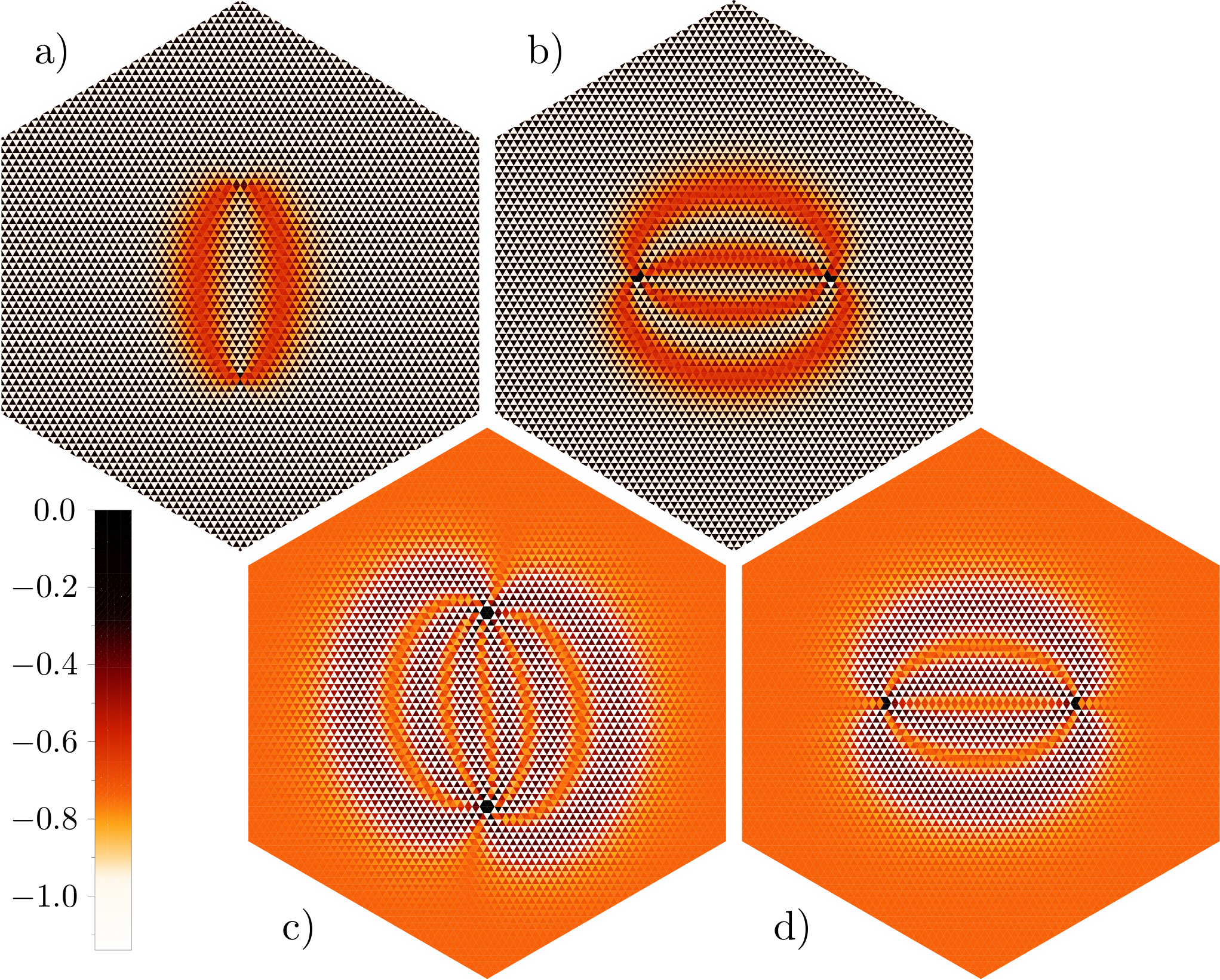
Next, we consider the other nematic phase with in which both O and C are spontaneously broken. Fig.2c shows the structure of a string connecting two charges separated along a line orthogonal to a lattice axis. First of all, the string now fractionalizes into six strands, which again separate alternating bulk phases. Interestingly, the interior of the strands consists of the bulk phase that occurs on the other side of the phase transition. As before, for the present arrangement of charges the symmetries R’ and CR are not explicitly broken. However, unlike in the nematic phase with , for not only CR but also R’ is spontaneously broken in the bulk, while the combination CRR’ remains unbroken. This explains the symmetry of the corresponding strand geometry. Two charges separated along a lattice axis are shown in Fig.2d. As before, in this situation both R and CR’ are not explicitly broken. However, unlike for , for neither R nor CR’ is spontaneously broken, which explains the reflection symmetries in the corresponding strand geometry.
Let us consider the static charge-anti-charge potential in the nematic confinement phase with for two charges separated along a lattice axis, as in Fig.2d. As expected, at large separation the potential is linearly rising, i.e. with the string tension (cf. Fig.3). As one approaches , becomes very small but does not go to zero, indicating again that the phase transition is weakly first order. The minimal value of is reached at the transition.
Finally, we realize the model as a quantum circuit that embodies the quantum link model on a chip. The dual formulation can also be used to perform real-time quantum simulations. Since the Gauss law constraint is partially resolved, this leads to a denser encoding of the physical Hilbert space than working with the fluxes themselves Bro19. Each dual height variable maps exactly to one qubit (). The electric field of eq.(3) is diagonal in this basis and is given in terms of the adjacent qubit operators as . While in the dual formulation there are no single link operators , operators for closed loops still exist. The plaquette operators , e.g., are given by four-qubit operators acting on the plaquette qubit and its three nearest neighbors . Exact cancellations in the full plaquette Hamiltonian yield at most three qubit interactions
| (6) | |||||
The real-time evolution is using a Trotter scheme which alternates between the plaquette terms on the and sublattices, while fully preserving Gauss’s law. Each sublattice Trotter step factorizes into mutually commuting single plaquette unitaries . Each factor translates into a very short gate sequence, as illustrated for in Fig.4, using eight two-qubit CNOT gates in combination with four single qubit rotations as well as two Hadamard gates for each plaquette.
This quantum circuit facilitates quantum computations of the string dynamics on a chip. Fig.5 shows an example of dynamics that can already be studied on today’s devices. Here the system is a parallelogram of 8 plaquettes with fixed boundary conditions on all external plaquettes (not shown in Fig.5). The system is initialized in the ground state of (the sum of all plaquette terms on sublattice (white triangles)), which happens to be a simple product state. The quenched dynamics using the full Hamiltonian at then leads to an oscillation between the order parameters of the two sublattices (cf. eq.(4)). This system also contains a flux string connecting fractional charges at the top and bottom corner. Initially that flux is wired along the left boundary, but it starts to oscillate along with the order parameters.
Another worthwhile phenomenon to study is the crossing of the quantum phase transition in real time. Fig.2 shows that the interior of the strands consists of the bulk phase that is realized on the other side of the transition, such that the string interior and the surrounding bulk must exchange their roles during this transition.
The rich string dynamics of the simple quantum link model provides additional motivation to push the experimental frontier forward in this direction, towards the ultimate goal of quantum simulating QCD itself Wie14.
The research leading to these results has received funding from the Schweizerischer Nationalfonds and from the European Research Council under the European Union’s Seventh Framework Programme (FP7/2007-2013)/ ERC grant agreement 339220.
References
- (1) M. Lüscher, K. Symanzik, P. Weisz, Nucl. Phys. B173 (1980) 365.
- (2) M. Lüscher, Nucl. Phys. B180 (1981) 317.
- (3) M. Lüscher, G. Münster, P. Weisz, Nucl. Phys. B180 (1981) 1.
- (4) M. Lüscher, P. Weisz, JHEP 0109 (2001) 010.
- (5) M. Lüscher, P. Weisz, JHEP 0207 (2002) 049.
- (6) K. J. Juge, J. Kuti, C. Morningstar, Phys. Rev. Lett. 90 (2003) 161601.
- (7) P. Majumdar, Nucl. Phys. B664 (2003) 213.
- (8) M. Lüscher, P. Weisz, JHEP 0407 (2004) 014.
- (9) B. B. Brandt, P. Majumdar, Phys. Lett. B682 (2009) 253.
- (10) F. Gliozzi, M. Pepe, U.-J. Wiese, Phys. Rev. Lett. 104 (2010) 232001.
- (11) B. B. Brandt, M. Meineri, Int. J. Mod. Phys. A31 (2016) 1643001.
- (12) D. Horn, Phys. Lett. B100 (1981) 149.
- (13) P. Orland, D. Rohrlich, Nucl. Phys. B338 (1990) 647.
- (14) S. Chandrasekharan, U.-J. Wiese, Nucl. Phys. B492 (1997) 455.
- (15) R. Brower, S. Chandrasekharan, U.-J. Wiese, Phys. Rev. D 60 (1999) 094502.
- (16) R. Brower, S. Chandrasekharan, S. Riederer, U.-J. Wiese, Nucl. Phys. B693 (2004) 149.
- (17) K. G. Wilson, Phys. Rev. D10 (1974) 2445.
- (18) D. Banerjee, F.-J. Jiang, P. Widmer, U.-J. Wiese, PoS LATTICE2013 (2014) 333.
- (19) D. Banerjee, F.-J. Jiang, P. Widmer, U.-J. Wiese, J. Stat. Mech. 1312 (2013) P12010.
- (20) D. Banerjee, F.-J. Jiang, T. Z. Olesen, P. Orland, U.-J. Wiese, Phys. Rev. B97 (2018) 205108.
- (21) N. Shannon, G. Misguich, K. Penc, Phys. Rev. B69 (2004) 220403.
- (22) L. Cardarelli, S. Greschner, L. Santos, Phys. Rev. Lett. 119 (2017) 180402.
- (23) Y.-P. Huang, D. Banerjee, M. Heyl, Phys. Rev. Lett. 122 (2019) 250401.
- (24) F. Tschirsich, S. Montangero, M. Dalmonte, SciPost Phys. 6 (2019) 028.
- (25) R. C. Brower, D. Berenstein, H. Kawai, PoS(LATTICE2019) 112.
- (26) T. Felser, P. Silvi, M. Collura, S. Montangero, Phys. Rev. X10 (2020) 041040.
- (27) L. Cardarelli, S. Greschner, L. Santos, Phys. Rev. Lett. 124 (2020) 123601.
- (28) A. Celi, B. Vermersch, O. Viyuela, H. Pichler, M. D. Lukin, P. Zoller, Phys. Rev. X10 (2020) 021057.
- (29) D. Luo, J. Shen, M. Highman, B. K. Clark, B. DeMarco, A. X. El-Khadra, B. Gadway, Phys. Rev. A102 (2020) 032617.
- (30) T. V. Zache, M. Van Damme, J. C. Halimeh, P. Hauke, D. Banerjee, arXiv:2104.00025.
- (31) F. M. Surace, P. P. Mazza, G. Giudici, A. Lerose, A. Gambassi, M. Dalmonte, Phys. Rev. X10 (2020) 021041.
- (32) Y.-T. Kang, C.-Y. Lo, S. Yin, P. Chen, Phys. Rev. A101 (2020) 023610.
- (33) J. C. Halimeh, R. Ott, I. P. McCulloch, B. Yang, P. Hauke, Phys. Rev. Research 2 (2020) 033361.
- (34) D. Banerjee, A. Sen, Phys. Rev. Lett. 126 (2021) 220601.
- (35) M. Van Damme, H. Lang, P. Hauke, J. C. Halimeh, arXiv:2104.07040.
- (36) D. S. Rokhsar, S. A. Kivelson, Phys. Rev. Lett. 61 (1988) 2376.
- (37) D. Banerjee, M. Bögli, C. P. Hofmann, F.-J. Jiang, U.-J. Wiese, Phys. Rev. B90 (2014) 245143.
- (38) D. Banerjee, M. Bögli, C. P. Hofmann, F.-J. Jiang, U.-J. Wiese, Phys. Rev. B94 (2016) 115120.
- (39) U.-J. Wiese, Annalen der Physik 525 (2013) 777.
- (40) M. C. Banuls et al., Eur. Phys. J. D74 (2020) 165.
- (41) D. Banerjee, M. Bögli, M. Dalmonte, E. Rico, P. Stebler, U.-J. Wiese, P. Zoller, Phys. Rev. Lett. 110 (2013) 125303.
- (42) D. Banerjee, M. Dalmonte, M. Müller, E. Rico, P. Stebler, U.-J. Wiese, P. Zoller, Phys. Rev. Lett. 109 (2012) 175302.
- (43) A. W. Glätzle, M. Dalmonte, R. Nath, I. Rousochatzakis, R. Moessner, P. Zoller, Phys. Rev. X4 (2014) 041037.
- (44) D. Marcos, P. Widmer, E. Rico, M. Hafezi, P. Rabl, U.-J. Wiese, P. Zoller, Ann. Phys. 351 (2014) 634.
- (45) E. A. Martinez, C. A. Muschik, P. Schindler, D. Nigg, A. Erhard, M. Heyl, P. Hauke, M. Dalmonte, T. Monz, P. Zoller, Nature 534 (2016) 516.
- (46) H. Bernien, S. Schwartz, A. Keesling, H. Levine, A. Omran, H. Pichler, S. Choi, A. S. Zibrov, M. Endres, M. Greiner, V. Vuleti, M. D. Lukin, Nature 551 (2017) 579.
- (47) N. Klco, E. F. Dumitrescu, A. J. McCaskey, T. D. Morris, R. C. Pooser, M. Sanz, E. Solano, P. Lougovski, M. J. Savage, Phys. Rev. A98 (2018) 032331.
- (48) H.-H. Lu, N. Klco, J. M. Lukens, T. D. Morris, A. Bansal, A. Ekström, G. Hagen, T. Papenbrock, A. M. Weiner, M. J. Savage, Phys. Rev. A100 (2019) 012320.
- (49) C. Schweizer, F. Grusdt, M. Berngruber, L. Barbiero, E. Demler, N. Goldman, I. Bloch, M. Aidelsburger, Nature Physics 15 (2019) 1168.
- (50) F. Görg, K. Sandholzer, J. Minguzzi, R. Desbuquois, M. Messer, T. Esslinger, Nature Physics 15 (2019) 1161.
- (51) A. Mil, T. V. Zache, A. Hegde, A. Xia, R. P. Bhatt, M. K. Oberthaler, P. Hauke, J. Berges, F. Jendrzejewski, Science 367 (2020).
- (52) B. Yang, H. Sun, R. Ott, H.-Y. Wang, T. V. Zache, J. C. Halimeh, Z.-S. Yuan, P. Hauke, J.-W. Pan, Nature 587 (2020) 392.
- (53) Y. Atas, J. Zhang, R. Lewis, A. Jahanpour, J. F. Haase, C. A. Muschik, arXiv:2102.08920.
- (54) D. Banerjee, arXiv:2101.03161.
- (55) B. B. Beard, U.-J. Wiese, Phys. Rev. Lett. 77 (1996) 5130.
- (56) T. Sentil, A. Vishwanath, L. Balents, S. Sachdev, M. P. A. Fisher, Science 303 (2004) 1490.
- (57) T. Sentil, L. Balents, S. Sachdev, A. Vishwanath, M. P. A. Fisher, Phys. Rev. B70 (2004) 144407.
- (58) B. Zhao, P. Weinberg, A. W. Sandvik, Nature Physics 15 (2019) 678.
- (59) V. Gorbenko, S. Rychkov, B. Zan, JHEP 10 (2018) 108.
- (60) U.-J. Wiese, Nucl. Phys. A931 (2014) 246.