Highly accurate potential energy curves for the hydrogen molecule ion

The Schrödinger equation and related problems can usually be written in the following manner,

where $P(x)$ and $Q(x)$ are arbitrary functions that admit expansions in powers of $x$, $P(x)=\sum_{k=-1}^{\infty}p_{k}x^{k}$, and $Q(x)=\sum_{k=-2}^{\infty}q_{k}x^{k}$ and depend on one or more parameters $\lambda_{i}$. In the case of the one-dimensional Schrödinger equation, for example, $P(x)=0$, and $Q(x)=2E-V(x)$. If $L(x)\sim x^{s}$ when $x\rightarrow 0$, with $s$ being an integer number, then the the regularized logarithmic derivative of $L$, i.e., the function

can be expanded in a Taylor series around $x=0$, i.e., $f(x)=\sum f_{j}x^{j}$, and satisfies the following Riccati equation,

A recurrence relation can be found that relates each $f_{j}$ with the preceding $f_{0},\ldots,f_{j-1}$, and these also depend on the same parameters as $Q(x)$ and $P(x)$.

We now consider an $[M/N]$ Padé approximant to $f(x)$, i.e., a quotient of polynomials of degrees $M$ and $N$,

such that the series expansion of both $f(x)$ and $[M/N](x)$ coincide up to order $M+N+1$. To each function $f(x)$, there is a unique $[M/N]$ Padé approximant, and there is a set of $M+N$ linear equations that relate the coefficients $a_{j}$, and $b_{j}$ with the $f_{j}$ coefficients. The RPM consists in choosing the parameters on which $P$ and $Q$ depend in such a way that $[M/N]$ matches an extra coefficient $f_{j}$, i.e., $[M/N](x)-f(x)=O(x^{M+N+2})$. This adds an extra equation to the set of $M+N$ ones, and it is straightforward to show that this set has a non-trivial solution if

where we have defined $D=N+1$, and $d=M-N$.

Eq. (5) provides a quantization condition for one of the parameters $\lambda_{1},\ldots,\lambda_{n}$ and allows to obtain it in terms of the others. For example, in the case of the one-dimensional Schrödinger equation, if the Hamiltonian depends on one parameter, then one can obtain the energy in terms of it, or the values of said parameter for which the energy adopts a particular value, as in the case of the critical parametersFernandez_2013. In the case of coupled equations (which is of concern in the present work), one should have as many coupled equations as unknown parameters, and Eq. (5) should be solved simultaneously for each of the equations. The quantization condition (5) is known to yield both the bound states and resonances of many problems in Quantum Mechanics, and it is believed it does so by sending a movable pole at complex infinity Abbasbandy:11. The singularity can be moved around any path in the complex plane, meaning that Eq. (5) also gives solution to both kinds of problems without specifying the boundary conditions Fernandez_1996; Fernndez2016.

Within the Born-Oppenheimer approximation, the electronic Hamiltonian for the H${}_{2}^{+}$ molecule is,

where $\nabla$ involves differentiation with respect to the electron coordinates, and $r_{1,2}$ are the absolute distances between the electron and each of the nuclei. Here atomic units are being used. The Schrödinger equation defined by Eq. (6) can be transformed into a set of separable equations by using the spheroidal coordinates $\lambda,\mu$ and $\phi$, where $\lambda$ and $\mu$ are defined as

and $0\leq\phi\leq 2\pi$ is the angle of rotation of the electron around the internuclear axis. $R$ is the internuclear separation, also in atomic units. The electronic wavefunction can be written as a product $\psi(\lambda,\mu,\phi)=L(\lambda)M(\mu)\Phi(\phi)$, and satisfies the following equations:

where $A$ is the separation constant, $\epsilon=-R^{2}E/2$, with $E$ being the electronic energy i.e., the eigenvalue of $H_{\rm mol}$, and $m$ is the quantum number associated with the angular momentum in the direction of the internuclear axis.

In order to solve Eqs. (10) and (11) with the RPM, we first define $x=\lambda-1$, which transforms Eq. (10) into Eq. (1), with

The solution $L(x)$ is known to behave at origin as $x^{|m|/2}$; then by setting $s=|m|/2$ in Eq. (2) we remove the singularities of Eq. (1) at origin, and writing $f(x)=\sum_{j=-1}^{\infty}f_{j}x^{j+1}$, the following recurrence relation for the coefficients $f_{j}$ is obtained,

where $p_{j}^{\lambda}$ and $q_{k}^{\lambda}$ are the expansion coefficients for $P_{\lambda}(x)$ and $Q_{\lambda}(x)$.

Similarly, by setting $\mu=x$, Eq. (11) transforms into Eq. (1), with

Now we define

Since $P_{\mu}(x)$ is odd and $Q_{\mu}(x)$ is even, $M(x)$ has defined parity. Therefore, $P_{\mu}(x)=\sum_{j=0}^{\infty}p_{j}^{\mu}x^{2j+1}$, $Q_{\mu}(x)=\sum_{j=0}^{\infty}q^{\mu}_{j}x^{2j}$, and $g(x)=\sum_{j=0}^{\infty}g_{j}x^{2j+t}$, where $t=0$ for even states and $1$ for odd states, and the following recurrence relation is obtained:

The RPM quantization condition (5) becomes

There are three unknowns and only two equations; consequently, equations (10) and (11) yield two parameters in terms of the third one. For benchmarking purposes, it is customary to solve for $\epsilon$ and $A$ in terms of $R$.

Any computer algebra system (CAS) contains subroutines to compute the determinant of a matrix. These subroutines are usually good enough for general purposes, but they don’t exploit the recurrence relation obeyed by the Hankel matrices that provides a much more efficient way to compute them,

where $H_{1}^{d}=f_{d+1}$, and we define $H_{0}^{d}=1$. To use Eq. (18), we start by computing coefficients $f_{d+1},\ldots,f_{2D+d-1}$. Then, we use them to compute $H_{2}^{d},\ldots,H_{2}^{2D+d-4}$; these are used to compute $H_{3}^{d},\ldots,H_{3}^{2D+d-6}$, and so on, until we reach $H_{D}^{d}$. Since only determinants of order $D-1$ and $D-2$ are needed to compute determinants of order $D$, for each step we only need to store two rows of determinants in memory. As an example, Figure 1 shows the sequence of determinants required to compute $H_{5}^{2}$.

Now we discuss the issue of solving Eqs. (17), i.e., finding the roots of the Hankel determinants. To that end, we resort to the well-known Newton-Raphson (NR) method, using numerical differentiation in the form of the symmetric difference quotient. One difficulty that may arise when finding the roots of the Hankel determinants is that $H_{D}^{d}$ presents multiple roots that approach to the eigenvalues of the problem Fernandez_1989c; Fernandez_1995. The reason for this is hinted at Eq. (18), by realizing that one solution for $H_{D}^{d}=0$ is $H_{D-1}^{d}H_{D-1}^{d+2}=(H_{D-1}^{d+1})^{2}$, but also if both $H_{D-1}^{d}$, $H_{D-1}^{d+2}$, and $H_{D-1}^{d+1}$ are close enough to 0 (they should be, since they are themselves the roots of another Hankel determinant), $H_{D}^{d}$ may also become 0. It is typically observed that different sequences of roots converge towards the desired eigenvalues with different speed; we call the fastest of them the “main sequence”. If the starting values provided for the NR method are not good enough it may converge to roots that are not in the main sequence, and for increasing $D$, the sequence of roots of $H_{D}^{d}$ may converge more slowly towards the desired eigenvalue. Besides, it is a well-known fact that the convergence of the NR method deteriorates when dealing with multiple roots. Despite these issues, we have been able to successfully compute the roots of the Hankel determinants for other problems in the past, and for the problem described here in particular, as will be shown below.

The simultaneous solution of Eqs. (17) allows for two different approaches. One of them is to choose a desired value of $R$, and then solve both equations simultaneously for $\epsilon$ and $A$. This implies solving a system of two equations with two unknowns, for which the NR method is very well suited, but each iteration of the method involves the evaluation of four derivatives. The other one is to set a value of $\epsilon$, then solve $H_{\mu,D}^{d}(\epsilon,A)$ to get the corresponding value of $A$, and solve $H_{\lambda,D}^{d}(\epsilon,A,R)=0$ for the value of $R$. The latter approach has the advantage that it is only required to solve two separate equations, instead of solving them simultaneously, so that it is only necessary to perform one differentiation per iteration for each equation. Unfortunately, the utility of the latter method is limited, since for benchmarking purposes it is usually more desirable to compute $\epsilon$ and $A$ values for selected values of $R$. In the present work we will use both approaches with different purposes, as discussed in the following sections.

The software developed to compute the roots of the Hankel determinants for the $H_{2}^{+}$ molecule is made available under a free software license; its location is disclosed in the Supplementary Material section below.

We first turn our attention to the rate at which the solutions of Eqs. (17) converge towards the correct values of $A$ and $\epsilon$ for different values of $R$. To do so, we first set a value of $R$ ($=1,2,5,10,20,50,$ or $90$), and then we pick an approximate value of the electronic energy $E$ from Ref. Madsen_1970 (the use of literature values is not strictly required, as discussed in the following section, but facilitates our work). We then compute $\epsilon=-R^{2}E/2$ and solve $H_{D,\mu}^{0}(\epsilon,A)=0$ for increasing values of $D$ (using $d=1,2$ gives similar results). To measure the convergence rate, we plot $\Delta=\log_{10}|(A[D,0]-A[D\raisebox{0.75pt}{-}1,0])/A[D,0]|$ against $D$, where $A[D,d]$ is the value of $A$ computed by solving $H_{\lambda,D}^{d}=0$. This plot gives a good approximation to the number of significant digits in the result. We proceed similarly to measure the convergence rate of the roots of $H_{\lambda,D}^{0}$ towards the value of $\epsilon$ that corresponds to the value of $R$ chosen at the beginning and the corresponding value of $A$ computed with $H_{\mu,D}^{0}=0$. We repeated this procedure for the states $1s\sigma_{g}$, $2p\sigma_{u}$, $2p\pi_{u}$, and $3d\delta_{g}$, which are the states with the lowest energy for the sets of quantum numbers $(m,s)$ equal to $(0,0)$, $(0,1)$, $(1,0)$, and $(1,1)$, respectively. The plots of $\Delta$ vs $D$ for the $\mu$- and $\lambda$- equations are shown in Figs. 2 and 3, respectively.

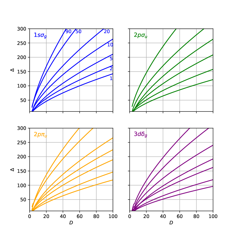
Figure 2 shows that for the four states analyzed, the smaller the values of $R$ (or $\epsilon$), the greater the rate of convergence. Remarkably, the later is faster than exponential, since the plot of the logarithmic difference between iterations is convex. An analysis of the plot for $\epsilon$ leads to the opposite conclusion, i.e., convergence rate is slower than exponential, and it increases for larger $R$. The result is that for larger (or smaller) values of $R$, solving both of equations (17) simultaneously can become more difficult, since the solution of one of the equations converges faster than the other one. Despite this, for the lower-lying states, convergence speed of both equations is fast enough to obtain accurate results without great computational effort, as shown in the following sections.

As discussed before, for the NR method to converge towards the roots of the Hankel determinants, it is important to provide good initial values. This usually implies computing approximate values using another method or looking them up in literature, but for this particular problem we have designed a very simple algorithm that allows to compute the electronic energy for any state of the H${}_{2}^{+}$ molecule without resorting to external references. To do so, it takes advantage of the fact that when $R=0$, both nuclei merge, transforming the system into He⁺, whose Schrödinger equation can be solved exactly. We refer to this case as the united-atom (UA) limit. The eigenvalue $E$ in the UA limit is equal to $-2/n_{u}^{2}$, where $n_{u}$ is the quantum number (note that $n_{u}$ is a “good” quantum number only in this limit). To identify each state for general $R$ and relate it to the UA ones, we follow Ref. Bates_1968 in using the quantum number $m$, and the “quantum numbers” $l$ and $I$. Here $l$ is the angular quantum number of the UA solution, and $I=n_{u}-l$ distinguishes states with the same $l$ but different $n_{u}$. The numbers of nodes of the solutions of equations (10) and (11) ($N_{\lambda}$ and $N_{\mu}$) are related to $I$ and $l$ according to $N_{\lambda}=I-1$, and $N_{\mu}=|l-m|$. As stated before, when computing the Hankel determinants, $s$ must be set to $|m|/2$, and $t$ must be set equal to $0$ if $N_{\mu}$ is even, and to $1$ if $N_{\mu}$ is odd. The separation constant $A$ in the UA limit is $A=-l(l+1)$ Scott_2006.

To compute the whole energy curve (and its corresponding separation constants), we begin from the UA limit ($R=0$), computing the corresponding values of $E$ and $A$ using the exact formulas. Then, we set $R\leftarrow R+\delta$, and use these values of $E$ and $A$ as starting points for the NR method to solve Eqs. (17) simultaneously, with $D=D_{\rm min}$, with $D_{\rm min}$ originally set to 5. The result is used as a starting point for $D=D_{\rm min}+1$, and so on, until $D=D_{\rm min}+10$. This yields results with a varying number of significant digits, depending on the rate at which Eqs. (17) converge towards the correct values, which can fluctuate significantly, as shown in Figs. 2 and 3. By comparing the amount of digits that coincide between the roots of Eqs. (17) for two subsequent values of $D$, one can estimate the number of digits of a given approximate result that are correct. For a given value of $D$, the Hankel determinant may not be large enough that its roots give an approximation to a particular state. For increasing $N_{\lambda}$ and $N_{\mu}$, usually larger values of $D$ are required, and if using a smaller value, the NR method converges to an approximation of a different state, or does not converge at all. This can be easily accounted for by comparing the converged result with the initial value provided to the NR method. If the relative difference between these values is greater than a set threshold, then the computation is repeated using a larger value of $D_{\rm min}$. The new values $E(R+\delta)$ and $A(R+\delta)$ can be used as starting values for $R+2\delta$, and the procedure is repeated until the desired values of $R$ are covered. For a given $R$, too large values of $\delta$ make $E$ and $A$ unsuitable starting points for the NR method to find the Hankel determinant roots for $R+\delta$. A much better starting point is provided by extrapolating the three previous values of $E$ and $A$ using a quadratic equation. We have included all the computations we performed in the Supplementary Material, with the correct amount of significant digits. The algorithm described above is also provided under a free software license in the form of a Python script.

As discussed in the Introduction, it is of interest to have accurate benchmark values available, mainly to use them as a test for other methods. Here we compute $E$ and $A$ for some electronic states at particular internuclear distances to a large number of digits. We do so by using as starting points the values computed in the previous section, and improve their accuracy by solving Eqs. (17) for values of $D$ from 2 to 100. Whenever we found that a result was accurate to 100 or more digits, we stopped the calculation to save time. Also, some of the computations were stopped earlier because the NR method was unable to find the roots after 10000 successive iterations. The values provided here may serve as benchmarks for testing other methods, and we would like to reiterate here that results of similar quality can be obtained for different internuclear positions and quantum numbers by using the software provided with the present work. For brevity, the complete results are not presented in this article, but they are provided in the Supplementary Material. Table 1 has a summary of all the computed states and the number of significant digits provided, maximum value of $D$ reached, and approximate values of $E$ and $A$.

Within the Born-Oppenheimer approximation, a minimum of a potential-energy curve is a necessary condition for bound states.

By inspecting several of the plots of $U(R)$ for different states, it is easy to realize that several of them exhibit a minimum. Fig. 4 shows $U(R)$ for all the binding states computed in the present work, with the exception of the ground state. As stated in Ref. Fernandez_1995, equilibrium distances, energies, and separation constants, can be computed by means of the RPM by solving the additional equation

where $F(U,A,R)=H_{\mu,D}^{d}(U,A,R)$, and $G(U,A,R)=H_{\lambda,D}^{d}(U,A,R)$.

Therefore, to obtain the equilibrium energy $U_{\rm eq}$, separation constant $A_{\rm eq}$, and internuclear distance $R_{\rm eq}$, we solve Eqs. (17) and (20) simultaneously. For the ground state, we found that it is better to solve instead for $H_{\lambda,2D}^{d}(U,A,R)$, since, for this particular set of parameters, the roots of the Hankel determinants converge faster towards the solution of Eq. (11) than Eq. (10). Analyzing those solutions with $D\leq 100$ for $d=0,1$, and $2$, we get the following results for the ground state:

We performed similar computations with $D\leq 50$ for the other bound states, and tabulated the results with 10 significant digits in Table 2. The same results are provided with 40 significant digits in the Supplementary Material.

References

- (1) D. R. Bates, K. Ledsham, and A. L. Stewart, “Wave functions of the hydrogen molecular ion,” Philosophical Transactions of the Royal Society of London. Series A, Mathematical and Physical Sciences, vol. 246, pp. 215–240, nov 1953.
- (2) J. M. Peek, “Eigenparameters for the 1s and 2p orbitals of H,” The Journal of Chemical Physics, vol. 43, pp. 3004–3006, nov 1965.
- (3) D. Bates and R. Reid, “Electronic eigenenergies of the hydrogen molecular ion,” in Advances in Atomic and Molecular Physics, pp. 13–35, Elsevier, 1968.
- (4) C. L. Beckel, B. D. Hansen, and J. M. Peek, “Theoretical study of H ground electronic state spectroscopic properties,” The Journal of Chemical Physics, vol. 53, pp. 3681–3690, nov 1970.
- (5) M. M. Madsen and J. M. Peek, “Eigenparameters for the lowest twenty electronic states of the hydrogen molecule ion,” Atomic Data and Nuclear Data Tables, vol. 2, pp. IN3–204, dec 1970.
- (6) P. Okun and K. Burke, “Uncommonly accurate energies for the general quartic oscillator,” International Journal of Quantum Chemistry, vol. 121, dec 2020.
- (7) A. V. Turbiner and J. C. del Valle, “Comment on: Uncommonly accurate energies for the general quartic oscillator, Int. J. Quantum Chem., e26554 (2020), by P.Okun and K.Burke,” arXiv e-prints, p. arXiv:2102.09246, Feb. 2021.
- (8) M. Braun, “Finite element calculations for systems with multiple coulomb centers,” Journal of Computational and Applied Mathematics, vol. 236, pp. 4840–4845, dec 2012.
- (9) D. M. Chipman and J. O. Hirschfelder, “Perturbation theories for the calculation of molecular interaction energies. II. application to H,” The Journal of Chemical Physics, vol. 59, pp. 2838–2857, sep 1973.
- (10) B. Jeziorski, K. Szalewicz, and G. Chałasiński, “Symmetry forcing and convergence properties of perturbation expansions for molecular interaction energies,” International Journal of Quantum Chemistry, vol. 14, pp. 271–287, sep 1978.
- (11) G. Chałasińaski and K. Szalewicz, “Degenerate symmetry-adapted perturbation theory. convergence properties of perturbation expansions for excited states of h ion,” International Journal of Quantum Chemistry, vol. 18, pp. 1071–1089, oct 1980.
- (12) S. Yamamoto, Y. Hatano, and H. Tatewaki, “Artificial nodes in the h wave functions expanded using gaussian-type orbitals or laguerre-type orbitals,” Computational and Theoretical Chemistry, vol. 1103, pp. 17–24, mar 2017.
- (13) Y. P. Sarwono, F. U. Rahman, and R. Zhang, “Numerical variational solution of hydrogen molecule and ions using one-dimensional hydrogen as basis functions,” New Journal of Physics, vol. 22, p. 093059, sep 2020.
- (14) R.-H. Xie and J. Gong, “Simple three-parameter model potential for diatomic systems: From weakly and strongly bound molecules to metastable molecular ions,” Physical Review Letters, vol. 95, dec 2005.
- (15) J. C. Xie, T. Kar, and R.-H. Xie, “An accurate pair potential function for diatomic systems,” Chemical Physics Letters, vol. 591, pp. 69–77, jan 2014.
- (16) K. Szalewicz, “Determination of structure and properties of molecular crystals from first principles,” Acc. Chem. Res., vol. 47, pp. 3266–3274, 2014.
- (17) M. P. Metz, K. Piszczatowski, and K. Szalewicz, “Automatic generation of intermolecular potential energy surfaces,” Journal of Chemical Theory and Computation, vol. 12, pp. 5895–5919, dec 2016.
- (18) M. W. Schmidt, J. Ivanic, and K. Ruedenberg, “Covalent bonds are created by the drive of electron waves to lower their kinetic energy through expansion,” The Journal of Chemical Physics, vol. 140, p. 204104, may 2014.
- (19) M. Beyer and F. Merkt, “Observation and calculation of the quasibound rovibrational levels of the electronic ground state of H,” Physical Review Letters, vol. 116, feb 2016.
- (20) M. Beyer and F. Merkt, “Structure and dynamics of H near the dissociation threshold: A combined experimental and computational investigation,” Journal of Molecular Spectroscopy, vol. 330, pp. 147–157, dec 2016.
- (21) S. Schiller, I. Kortunov, M. H. Vera, F. Gianturco, and H. da Silva, “Quantum state preparation of homonuclear molecular ions enabled via a cold buffer gas: An ab initio study for the H and the D case,” Physical Review A, vol. 95, apr 2017.
- (22) H. Olivares-Pilón and A. V. Turbiner, “The H molecular ion: Low-lying states,” Annals of Physics, vol. 373, pp. 581–608, oct 2016.
- (23) V. M. Khmara, M. Hnatič, V. Y. Lazur, and O. K. Reity, “Quasicrossings of potential curves in the two-coulomb-center problem,” The European Physical Journal D, vol. 72, feb 2018.
- (24) T. J. Price and C. H. Greene, “Semiclassical treatment of high-lying electronic states of H,” The Journal of Physical Chemistry A, vol. 122, pp. 8565–8575, oct 2018.
- (25) H. de Oliveira Batael and E. D. Filho, “Excited states for hydrogen ion molecule confined by a prolate spheroidal boxes: variational approach,” Theoretical Chemistry Accounts, vol. 139, jul 2020.
- (26) B. D. B. Figueiredo and M. Novello, “Solutions to a spheroidal wave equation,” Journal of Mathematical Physics, vol. 34, pp. 3121–3132, jul 1993.
- (27) B. D. B. Figueiredo, “Generalized spheroidal wave equation and limiting cases,” Journal of Mathematical Physics, vol. 48, p. 013503, jan 2007.
- (28) R. Boyack and J. Lekner, “Confluent heun functions and separation of variables in spheroidal coordinates,” Journal of Mathematical Physics, vol. 52, p. 073517, jul 2011.
- (29) T. Kereselidze, G. Chkadua, and P. Defrance, “Coulomb sturmians in spheroidal coordinates and their application for diatomic molecular calculations,” Molecular Physics, vol. 113, pp. 3471–3479, apr 2015.
- (30) T. Kereselidze, G. Chkadua, P. Defrance, and J. F. Ogilvie, “Derivation, properties and application of coulomb sturmians defined in spheroidal coordinates,” Molecular Physics, vol. 114, pp. 148–161, oct 2015.
- (31) T. C. Scott, M. Aubert-Frécon, and J. Grotendorst, “New approach for the electronic energies of the hydrogen molecular ion,” Chemical Physics, vol. 324, pp. 323–338, may 2006.
- (32) G. Hadinger, M. Aubert-Frecon, and G. Hadinger, “The killingbeck method for the one-electron two-centre problem,” Journal of Physics B: Atomic, Molecular and Optical Physics, vol. 22, pp. 697–712, mar 1989.
- (33) F. M. Fernandez, G. I. Frydman, and E. A. Castro, “Tight bounds to the schrodinger equation eigenvalues,” Journal of Physics A: Mathematical and General, vol. 22, pp. 641–645, mar 1989.
- (34) F. M. Fernández, Q. Ma, D. J. DeSmet, and R. H. Tipping, “Calculation of energy eigenvalues via supersymmetric quantum mechanics,” Canadian Journal of Physics, vol. 67, pp. 931–934, oct 1989.
- (35) F. M. Fernández, Q. Ma, and R. H. Tipping, “Eigenvalues of the schrödinger equation via the riccati-padé method,” Physical Review A, vol. 40, pp. 6149–6153, dec 1989.
- (36) F. M. Fernández, Q. Ma, and R. H. Tipping, “Tight upper and lower bounds for energy eigenvalues of the schrödinger equation,” Physical Review A, vol. 39, pp. 1605–1609, feb 1989.
- (37) F. M. Fernández, “Strong coupling expansion for anharmonic oscillators and perturbed coulomb potentials,” Physics Letters A, vol. 166, pp. 173–176, jun 1992.
- (38) F. M. Fernández, R. Guardiola, and M. Znojil, “Riccati-padé quantization and oscillatorsV(r)=grα,” Physical Review A, vol. 48, pp. 4170–4174, dec 1993.
- (39) F. M. Fernández, “Alternative treatment of separable quantum-mechanical models: The hydrogen molecular ion,” The Journal of Chemical Physics, vol. 103, pp. 6581–6585, oct 1995.
- (40) F. M. Fernández and J. Garcia, “Unitary transformations of a family of two-dimensional anharmonic oscillators,” Journal of Mathematical Chemistry, vol. 54, pp. 1321–1326, mar 2016.
- (41) F. M. Fernández and J. Garcia, “Highly accurate calculation of the real and complex eigenvalues of one–dimensional anharmonic oscillators,” Acta Polytechnica, vol. 57, p. 391, dec 2017.
- (42) F. M. Fernández and J. Garcia, “Highly accurate calculation of the resonances in the stark effect in hydrogen,” Applied Mathematics and Computation, vol. 317, pp. 101–108, jan 2018.
- (43) F. M. Fernández, “Quantization condition for bound and quasibound states,” Journal of Physics A: Mathematical and General, vol. 29, pp. 3167–3177, jun 1996.
- (44) F. M. Fernández and J. Garcia, “On two different kinds of resonances in one-dimensional quantum-mechanical models,” Journal of Mathematical Chemistry, vol. 55, pp. 623–631, oct 2016.
- (45) F. M. Fernández and J. Garcia, “Local approximation to the critical parameters of quantum wells,” Applied Mathematics and Computation, vol. 220, pp. 580–592, sep 2013.
- (46) S. Abbasbandy and C. Bervillier, “Analytic continuation of Taylor series and the boundary value problems of some nonlinear ordinary differential equations,” Applied Mathematics and Computation, vol. 218, pp. 2178–2199, nov 2011.