Tight Mutual Information Estimation With Contrastive Fenchel-Legendre Optimization
Abstract
Successful applications of InfoNCE (Information Noise-Contrastive Estimation) and its variants have popularized the use of contrastive variational mutual information (MI) estimators in machine learning. While featuring superior stability, these estimators crucially depend on costly large-batch training, and they sacrifice bound tightness for variance reduction. To overcome these limitations, we revisit the mathematics of popular variational MI bounds from the lens of unnormalized statistical modeling and convex optimization. Our investigation yields a new unified theoretical framework encompassing popular variational MI bounds, and leads to a new simple and powerful contrastive MI estimator we name FLO. Theoretically, we show that the FLO estimator is tight, and it converges under stochastic gradient descent. Empirically, the FLO estimator overcomes the limitations of its predecessors and learns more efficiently. The utility of FLO is verified using extensive benchmarks, and we further inspire the community with novel applications in meta-learning. Our presentation underscores the foundational importance of variational MI estimation in data-efficient learning.
1 Introduction
Assessing the dependence between pairs of variables is integral to many scientific and engineering endeavors [69, 70]. Mutual information (MI) is a popular metric to quantify generic associations [53], and its empirical estimators have been widely used in applications such as independent component analysis [8], fair learning [34], neuroscience [61], Bayesian optimization [47], among others. Notably, the recent advances in deep self-supervised learning (SSL) heavily rely on nonparametric MI optimization [76, 60, 38, 19, 32]. In this study we investigate the likelihood-free variational approximation of MI using only paired samples, and improve the data-efficiency of current machine learning practices.
MI estimation has been extensively studied [11, 54, 53, 62, 64, 77]. While most classical estimators work reasonably well for low-dimensional cases, they scale poorly to big datasets: naïve density-based estimator(s) and -nearest neighbor estimators [49, 63, 27] struggle with high-dimensional inputs, while kernel estimators are slow, memory demanding and sensitive to hyperparameters [31, 30]. Moreover, these estimators are usually either non-differentiable or need to hold all data in memory. Consequently, they are not well suited for emerging applications where the data representation needs to be differentiably optimized based on small-batch estimation of MI [42]. Alternatively, one can approach MI estimation through an estimated likelihood ratio [73, 42], but the associated numerical instability has raised concerns [6].
To scale MI estimation to the growing size and complexity of modern datasets, and to accommodate the need for representation optimization [14], variational objectives have been widely utilized recently [60]. Instead of directly estimating data likelihoods, density ratios, or the corresponding gradients [81], variational approaches appeal to mathematical inequalities to construct tractable lower or upper bounds of the mutual information [65], facilitated by the use of auxiliary critic functions11 1 When estimates are sharp, these critic functions usually recover some transformation of the likelihood ratio.. This practice turns MI estimation into an optimization problem. Prominent examples include the Barber-Agakov (BA) estimator [9], the Donsker-Varadhan (DV) estimator [21], and the Nguyen-Wainwright-Jordan (NWJ) estimator [58]. These variational estimators are closely connected to the variational objectives for likelihood inference [1].
Despite reported successes, these variational estimators have a major limitation: their estimation variance grows exponentially to the ground-truth MI [55]. This is especially harmful to applications involving deep neural nets, as it largely destabilizes training [72]. An effective fix is to leverage multi-sample contrastive estimators, pioneered by the work of InfoNCE [60]. However, the massive reduction in the variance comes at a price: the performance of the InfoNCE estimator is upper bounded by , where is the number of negative samples used [65]. For a large MI, needs to be sufficiently large to allow for an adequate estimate, consequently placing a significant burden on computation and memory. While variants of InfoNCE have been motivated to achieve more controllable bias and variance tradeoffs [65, 72], little research has been conducted on the cost-benefit aspect of contrastive learning.

A critical insight enabled by InfoNCE is that mutual information closely connects to contrastive learning [35, 60]. Paralleled by the empirical successes of instance discrimination-based self-supervision [56, 83, 19, 38] and multi-view supervision [75, 66], InfoNCE offers an InfoMax explanation to why the ability to discriminate naturally paired positive instances from the randomly paired negative instances leads to universal performance gains in these applications [51, 71, 65]. Despite these encouraging developments, the big picture of MI optimization and contrastive learning is not yet complete: () There is an ongoing debate about to what extent MI optimization helps to learn [79]; () how does the contrastive view reconcile with those non-contrastive MI estimators; crucial for practical applications, () are the empirical tradeoffs made by estimators such as InfoNCE absolutely necessary? And theoretically, () formal guarantees on the statistical convergence of popular variational non-parametric MI estimation are missing currently.
In this work we seek to bridge the above gaps by approaching the MI estimation from the novel perspective of energy modeling. While this subject has recently been studied extensively using information-theoretic and variational inequalities, we embrace a new view from the lens of unnormalized statistical modeling. Our main contributions include:
- •
Unifying popular variational MI bounds under unnormalized statistical modeling;
- •
Deriving a simple but powerful novel contrastive variational bound called FLO;
- •
Providing theoretical justification of the FLO bound (tightness and convergence);
- •
Demonstrating strong empirical evidence of the superiority of FLO over its predecessors.
- •
Highlighting the importance of MI in data-efficient learning with novel applications
We contribute in-depth discussion to bridge the gaps between contrastive learning and MI estimation, along with principled practical guidelines informed by theoretical insights.
2 Fenchel-Legendre Optimization for Mutual Information Estimation
2.1 Preliminaries
This section briefly reviews the mathematical background needed for our subsequent developments.
Unnormalized statistical modeling defines a rich class of models of general interest. Specifically, we are interested in problems for which the system is characterized by an energy function , where is the system parameters and is known as the potential function. The goal is to find a solution that is defined by a normalized version of , i.e., , where is the loss function, is the base measure on and is called the partition function for . Problems in the above form arise naturally in statistical physics [68], Bayesian analysis [15], and maximal likelihood estimation [74]. A major difficulty with unnormalized statistical modeling is that the partition function is generally intractable for complex energy functions 22 2 In the sense that they do not render closed-from expressions., and in many applications is further composed by , whose concavity implies any finite sample estimate Monte-Carlo of will render the loss function biased [67, 88]. Bypassing the difficulties caused by the intractable partition function is central to unnormalized statistical modeling [29, 57, 40, 43, 35].
Mutual information and unnormalized statistical models. As a generic score assessing the dependency between two random variables , mutual information is formally defined as the Kullback-Leibler divergence (KL) between the joint distribution and product of the respective marginals [70], i.e., . The integrand is often known as the point-wise mutual information (PMI) in the literature. Mutual information has a few appealing properties: () it is invariant wrt invertible transformations of and , and () it has the intuitive interpretation of reduced uncertainty of one variable given another variable33 3 Formally, , where (resp. ) denotes the Shannon entropy (resp. conditional Shannon entropy) of a random variable..
To connect MI to unnormalized statistical modeling, we consider the classical Barber-Agakov (BA) estimator of MI [10]. To lower bound MI, BA introduces a variational approximation for the posterior , and by rearranging the terms we obtain an inequality
| (1) | |||||
Here we have used notation to highlight the dependence on , and when this bound is sharp. Unfortunately, this naïve BA bound is not useful for sample-based MI estimation, as we do not know the ground-truth . But we can bypass this difficulty by setting , where we call the tilting function and recognize as the associated partition function. Substituting this into (S18) gives the following unnormalized BA bound (UBA) that pertains to unnormalized statistical modeling [65]
| (2) |
While this UBA bound remains intractable, now with instead of we can apply different techniques for empirical estimates of to render a tractable surrogate target. This has led to various popular MI bounds listed in Table 1 (see Appendix A for derivations).
InfoNCE and noise contrastive estimation. InfoNCE is a multi-sample mutual information estimator proposed in [60], built on the idea of noise contrastive estimation (NCE) [35]. NCE learns statistical properties of a target distribution by comparing the positive samples from the target distribution to the “negative” samples from a carefully crafted noise distribution, and this technique is also known as negative sampling in some contexts [56, 33]. The InfoNCE estimator implements this contrastive estimation idea via using the naïve empirical estimate of in UBA44 4 This estimator is technically equivalent to the original definition due to the symmetry of samples., i.e.
| (3) |
where is known as the critic in the nomenclature of contrastive learning, and we have used to denote independent draws from the joint density , and for each pair of samples. Here the positive and negative samples are respectively drawn from the joint and product of marginals . Intuitively, InfoNCE tries to accurately classify the positive samples when they are mixed with negative samples, and the Proposition below formally characterizes InfoNCE’s statistical properties as a MI estimator.
Proposition 2.1 ([65]).
InfoNCE is an asymptotically tight mutual information lower bound, i.e. ,
Fenchel-Legendre duality. Our key idea is to exploit the convex duality for MI estimation. Let be a proper convex, lower-semicontinuous function; then its convex conjugate function is defined as , where is the domain of function [41]. We call the Fenchel conjugate of , which is also known as the Legendre transform in physics. The Fenchel conjugate pair are dual to each other, in the sense that , i.e., For and its Fenchel conjugate , we have inequality
| (4) |
with the equality holds when .

2.2 Fenchel-Legendre Optimization for tight mutual information estimation
With the above mathematical tools, we are ready to present the main result of this paper: a tight, data-efficient variational MI lower bound that can be efficiently implemented.
Lower bounding MI with Fenchel-Legendre Optimization. Our key insight is that MI estimation is essentially an unnormalized statistical model, which can be efficiently handled by the Fenchel-Legendre transform technique. Take the integrand from UBA in (S21) and we can rewrite it as
| (5) |
where is the same probability density as (i.e., is an independent copy of ). Now let us use the Fenchel inequality of from (4), plugging it into the above equation and then we have
| (6) |
for all . This implies for any function , the following inequality holds
| (7) |
By putting (7) back to (S21), we obtain our new Fenchel-Legendre Optimization (FLO) MI lower bound
| (8) |
and concludes the proof for the following Proposition.
Proposition 2.2.
.
In practice, FLO can be estimated with the following naïve empirical -sample estimator
| (9) |
Since the summation in is not encapsulated by a convex transformation, is an unbiased estimator for independent of the batch size (see Figure 2).
Why is the FLO bound more appealing? At first sight, it may appear counter-intuitive that is a better MI bound compared to prior arts such as NWJ or InfoNCE: it seems to be more complicated as an extra variational function has been introduced. To answer this question, we next explain the statistical meaning of the newly introduced , and establish some important statistical properties of FLO that makes it more favorable: that is tight, meaning the ground-truth MI can be recovered for some specific choice of and ; and that for any batch size is effectively optimizing InfoNCE with an infinite batch size. And in Sec 2.4, we further justify FLO’s advantages from optimization perspectives.
Given the close connection between FLO and UBA, we first recall UBA’s optimal critic that gives the tight MI estimate is , where this can be any function of [52]. This is not directly meaningful in a statistical sense, however, by integrating out , we have
| (10) |
which is the likelihood ratio between the marginals and joint. On the other hand, based on the Fenchel-Legendre inequality (4), we know for fixed our FLO bound in (8) can be maximized with . Putting these all together we have This shows the introduced in FLO actually tries to recover the negative PMI. Comparing to the competing MI bounds that only optimizes for , eliminating the drift term reveals FLO enjoys the appealing self-normalizing property [35] that helps stabilize training. Plugging into (8), we readily see , proving FLO is a tight MI bound.
Proposition 2.3.
The FLO estimator is tight, the eqaulity holds when for arbitrary function and .
Corollary 2.4.
Let be the maximizers for (8), then .
Finally, we give a simple asymptotic argument showing FLO essentially optimizes InfoNCE with an infinite batch size. In virtue of the law of large numbers, we have the denominator in InfoNCE converging to , and consequently it recovers the UBA bound. Since FLO is derived from UBA, we can view FLO as using the optimization of to amortize the difficulty of evaluating infinite number of with InfoNCE.
Efficient implementations of FLO. A lingering concern is that the newly introduced can incur extra computation overhead. This is not true, as we can maximally encourage parameter sharing by jointly model and with a single neural network with two output heads, i.e., . Consequently, while FLO adopts a dual critics design, it does not actually invoke extra modeling cost compared to its single-critic counterparts (e.g., InfoNCE). Experiments show this shared parameterization in fact promotes synergies and speeds up learning (see our ablation studies in Appendix).
To further enhance the computation efficiency, we consider a massively parallelized bi-linear critic design that uses all in-batch samples as negatives. Let , where and are respectively encoders that map data to unit sphere embedded in , is the inner product operation, and is the inverse temperature parameter. Thus the evaluation of the Gram matrix , where is a mini-batch of -paired samples and , can be parallelized via matrix multiplication. In this setup, the diagonal terms of are the positive scores while the off-diagonal terms negative scores. A similar strategy has been widely employed in the contrastive representation learning literature (e.g., [19])55 5 As an important note to the community, most open source implementations for the bilinear contrastive loss have mechanically implemented following the practice from pioneering contrastive learning studies, which is numerically unstable compared to our parameterization proposed here.. We can simply model the PMI critic as , whose computation cost is almost neglectable in practice, where feature encoders dominate computing.
2.3 Connections to the existing MI bounds
Due to space limitations, we elaborate the connections to the existing MI bounds here, and have relegated an extended related work discussion in a broader context to the Appendix.
From -partition approximation to MI bounds. To embrace a more holistic understanding, we list popular variational MI bounds together with our FLO in Table 1, and visualize their connections in Figure 1. With the exception of JSD, these bounds can be viewed from the perspective of unnormalized statistical modeling, as they differ in how the partition function is estimated. We broadly categorize these estimators into two families: the -family (DV, MINE, InfoNCE) and the exponential-family (NWJ, TUBA, FLO). In the -family, DV and InfoNCE are multi-sample estimators that leverage direct Monte-Carlo estimates for , and these two differ in whether to include the positive sample in the denominator or not. To avoid the excessive in-batch computation of the normalizer and the associated memory drain, MINE further employed an exponential moving average (EMA) to aggregate the normalizer across batches. Note for the -family estimators, their variational gaps are partly caused by the -transformation on finite-sample average due to Jensen’s inequality (i.e., ). In contrast, the objective of exponential-family estimators do not involve such -transformation, since they can all be derived from the Fenchel-Legendre inequality: NWJ directly applies the Fenchel dual of -divergence for MI [59], while TUBA exploits this inequality to compute the partition . Motivated from a contrastive view, our FLO applies the Fenchel-Legendre inequality to the -partition of contrast scores.
A contrastive view for MI estimation. The MI estimators can also be categorized based on how they contrast the samples. For instance, NWJ and TUBA are generally considered to be non-contrastive estimators, as their objectives do not compare positive samples against negative samples on the same scale (i.e., versus ), and this might explain their lack of effectiveness in representation learning applications. For JSD, it depends on a two-stage estimation procedure similar to that in adversarial training to assess the MI, by explicitly contrasting positive and negative samples to estimate the likelihood ratio. This strategy has been reported to be unstable in many empirical settings. The -family estimators can be considered as a multi-sample, single-stage generalization of JSD. However, the DV objective can go unbounded thus resulting in a large variance, and the contrastive signal is decoupled by the EMA operation in MINE. Designed from contrastive perspectives, InfoNCE trades bound tightness for a lower estimation variance, which is found to be crucial in representation learning applications. Our FLO formalizes the contrastive view for exponential-family MI estimation, and bridges existing bounds: the PMI normalizer is a more principled treatment than the EMA in MINE, and compared to DV the positive and negative samples are explicitly contrasted and adaptively normalized.
Important FLO variants. We now demonstrate that FLO is a flexible framework that not only recovers existing bounds, but also derives novel bounds such as
| (11) |
Recall the optimal and , which motivates us to parameterize in the form of , where models the arbitrary drift , and this recovers the TUBA bound. Additionally, we note that () fixing either of and , and optimizing the other also gives a valid lower bound to MI; and () a carefully chosen multi-input can be computationally appealing. As a concrete example, if we set to and update while artificially keeping the critic fixed 66 6 That is to say in is an independent copy of ., then FLO falls back to DV. Alternatively, we can consider the Fenchel dual version of it: using the same multi-input above, treat as fixed and only update , and this gives us the novel MI objective in (11), we call it Fenchel-Donsker-Varadhan (FDV) estimator.
2.4 Gradient and convergence analysis of FLO
In this section, we will establish that FLO better optimizes the MI because its gradient is more accurate than competing variational bounds such as NWJ and TUBA; also, we provide the first convergence analysis for variational MI estimation by showing FLO converges under SGD.
First, recall most tractable variational MI bounds are derived from and upper bounded by the intractable UBA bound [65]. For instance, with the same critic we have . So if we can show then FLO is better optimized. To simplify notations, we denote and , and we can easily verify
| (12) |
Since for fixed the corresponding optimal maximizing is given by (using (4)), we see that the term is essentially optimized to approximate . To emphasize this point, we now write . When this approximation is sufficiently accurate (i.e., ), we can see that approximates as follows
| (13) |
We can prove FLO will converge under much weaker conditions, even when this approximation is rough. The intuition is as follows: in (13), the term only rescales the gradient, so the optimizer is still proceeding in the same direction as UBA in SGD. The informal version of our result is summarized in the Proposition below (see the Appendix for the formal version and proof).
Proposition 2.5 (Convergence of FLO, informal version).
Let be the stochastic Robbins-Monro sequence of learning rates: and . If is bounded between (), then under the stochastic gradient descent scheme described in Algorithm 1, converges to a stationary point of with probability , i.e., . Additionally assume is convex with respect to , then FLO converges with probability to the global optimum of from any initial point .
Importantly, this marks the first convergence result for variational MI estimators. The convergence analyses for MI estimation is non-trivial and scarce even for those standard statistical estimators [62, 27, 67]. The lack of convergence guarantees has led to a proliferation of unstable MI-estimators used in practice (in particular, DV, JSD, and MINE) that critically rely on various empirical hacks to work well (see discussions in [72]). Our work establishes a family of variational MI estimators that provably converges, a contribution we consider significant as it fills an important gap in current literature on both theoretical and practical notes.

3 Experiments
We consider an extensive range of tasks to validate FLO and benchmark it against state-of-the-art solutions. To underscore the practical significance of MI in efficient machine learning, we demonstrate example applications from data collection (in statistical parlance, experimental design), self-supervised pre-training, to meta/transfer-learning. Limited by space, we present only the key results in the main text, and defer ablation studies and details of our experimental setups to the Appendix. Our code is available from https://github.com/qingguo666/FLO. All experiments are implemented with PyTorch.
Comparison to baseline MI bounds. We start by comparing FLO to the following popular competing variational estimators: NWJ, TUBA, and InfoNCE. We use the bilinear critic implementation for all models which maximally encourages both sample efficiency and code simplicity, and this strategy does perform best based on our observations. We consider the synthetic benchmark from [65], where is jointly standard Gaussian with diagonal cross-correlation parameterized by . We report and here (other studies only report up to , which is less challenging.), providing a reasonable coverage of the range of MI one may encounter in empirical settings.

To focus on the bias-variance trade-off, we plot the decimal quantiles in addition to the estimated MI in Figure 3, where FLO significantly outperformed its variational counterparts in the more challenging high-MI regime. In Figure 5, we show FLO also beats classical MI estimators [49, 80, 28]. In the Appendix I, we further discuss recent works on parametric estimators [20, 16] and alternative information metrics [85].
Bayesian optimal experiment design (BOED). We next direct our attention to BOED, a topic of significant interest shared by the statistical and machine learning communities [17, 82, 39, 26]. The performance of machine learning models crucially relies on the quality of data supplied for training, and BOED is a principled framework that optimizes the data collection procedure (in statistical parlance, conducting experiments) [25]. Mathematically, let be the data to be collected, be the parameters to be inferred, and be the experiment parameters the investigator can manipulate (a.k.a, the design parameters), BOED tries to find the optimal data collection procedure that is expected to generate data that is most informative about the underlying model parameters, i.e., solves for . In this study, we focus on the more generic scenario where explicit likelihoods are not available, but we can still sample from the data generating procedure [47, 48].
We consider three carefully-selected models from recent literature for their progressive practical significance and the challenges involved [24, 44, 46]: static designs of () a simple linear regression model and () a complex nonlinear pharmacokinetic model for drug development; and the dynamic policy design for () epidemic disease surveillance and intervention (e.g., for Covid-19 modeling). Designs with higher MI are more favorable, because it implies the data carries more information. In Figure 4 we compare design optimization curves using different MI optimization strategies, where FLO consistently leads. Popular NWJ and InfoNCE reports different tradeoffs that are less susceptible to FLO. We also examine the FLO predicted posteriors and confirm they are consistent with the ground-truth parameters (Figure 6 right). For the dynamic policy optimization, we also manually inspect the design strategies reported by different models (Figure 6 left,middle). Consistent with human judgement, FLO policy better assigns budgeted surveillance resources at different stages of pandemic progression.
A novel meta-learning framework. A second application of our work is to meta-learning, an area attracting substantial recent interest. In meta-learning, we are concerned with scenarios that at training time, there are abundant different labelled tasks, while upon deployment, only a handful of labeled instances are available to adapt the learner to a new task. Briefly, for an arbitrary loss , where is the task identifier and is the prediction made by the model, we denote the risk by . Denote as the expected risk for all tasks and for the mean of empirical risks computed from all training tasks. Inspired by recent information-theoretic generalization theories [84], we derived a novel, principled objective
| (14) |
where is known given the data size and loss function, are respectively data and task embeddings for training data, which for the first time lifts contrastive learning to the task and data distribution level. Our reasoning is that theoretically bounds from above, and it is relatively sharp for being data-dependent. We give more information on this in the Appendix and defer a full exposition to a dedicated paper due to independent interest and space limits here. Note other MI bounds are not suitable for this task due to resource and vari-
| Model | InfoNCE | SpecNCE [36] 77 7 Note SpecNCE does not explicitly target mutual information | FLO | FDV |
|---|---|---|---|---|
| MI |
ance concerns. In Figure 7 we show Meta-FLO wins big over the state-of-the-art model agnostic meta-learning (MAML) model on the regression benchmark from [23].
Self-supervised learning (SSL). Finally, we wrap our experiments with one of the prime applications of contrastive MI estimation in machine learning: SSL for model pre-training. Here we focus on how FLO-inspired objectives can improve the current practice of SSL, and given this topic’s independent interest, we defer in-depth discussions in our dedicated work [18] where SSL-specific problems such as training diagnosis and low-precision numerical overflow are explored in detail. In this experiment, we follow the SSL setup described in the SimCLR paper [19]: in the pre-training phase, we optimize the mutual information between difference augmentations of the same image (i.e., scaling, rotation, color jitting, etc.); and use linear probing accuracy as our perfromance criteria. We compare the effectiveness of the InfoNCE-based SimCLR framework [19] to our FLO-based alternatives. To ensure fair comparison, we have used the FDV variant defined in Eq. (11) as our training objective, so that we are not introducing extra parameters to model . We call our new model FlatCLR because, perhaps counter-intuitively, the second term in Eq. (11) contributing all the learning signal is constant one in value (i.e., being flat). In Figure 10 and 10, we show our new model FlatCLR shows superior sample efficiency compared to the SOTA SimCLR (a boost for the same performance, FlatCLR- versus SimCLR-). This result is significant because SimCLR’s crucial reliance on large-batch training is a well-known limitation [36, 86, 50]. Figure 10 shows typical training curves with the respective models. Note that while the empirical estimates of MI are tied between the two methods, FDV optimized representation enjoys a better ground-truth MI 88 8 Ground-truth MI is approximated by InfoNCE using a very large negative sample pool ( mini-batch)., which can be explained by its robustness to the numerical overflow issue (see [18] for details). Further comparisons on the ground-truth MI estimation with different estimators can be found in Table 7.
4 Conclusion
We have described a new framework for the contrastive estimation of mutual information from energy modeling perspectives. Our work not only encapsulates popular variational MI bounds but also inspires novel objectives such as FLO and FDV, which comes with strong theoretical guarantees. In future work, we will leverage our theoretical insights to improve practical applications involving MI estimation, such as representation learning, fairness, and in particular, data efficient learning.
Acknowledgements
The authors would like to thank the anonymous reviewers for their insightful comments. Q Guo gratefully appreciate the support of Amazon Fellowship. X Deng would like to thank the Advanced Research Computing program at Virginia Tech and Virginia’s Commonwealth Cyber Initiative (CCI) AI testbed for providing computational resources, also appreciate the CCI and CCI-Coastal grants to Virginia Tech. Part of this work is done before C Tao joined Amazon, and he was funded by National Science Foundation Grant No. 1934964. This work used the Extreme Science and Engineering Discovery Environment (XSEDE), which is supported by National Science Foundation grant number ACI-1548562 [78] and used the Extreme Science and Engineering Discovery Environment (XSEDE) PSC Bridges-2 and SDSC Expanse at the service-provider through allocation TG-ELE200002 and TG-CIS210044.
References
- [1] Alexander Alemi, Ben Poole, Ian Fischer, Joshua Dillon, Rif A Saurous, and Kevin Murphy. Fixing a broken ELBO. In ICML, pages 159–168, 2018.
- [2] Alexander A Alemi, Ian Fischer, Joshua V Dillon, and Kevin Murphy. Deep variational information bottleneck. In ICLR, 2016.
- [3] Linda JS Allen. A primer on stochastic epidemic models: Formulation, numerical simulation, and analysis. Infectious Disease Modelling, 2(2):128–142, 2017.
- [4] Linda JS Allen, Fred Brauer, Pauline Van den Driessche, and Jianhong Wu. Mathematical epidemiology, volume 1945. Springer, 2008.
- [5] Anonymous. Meta-flo: Principled simple fast few-shot learning with stochastic prompt encoding networks. 2022.
- [6] Martin Arjovsky and Léon Bottou. Towards principled methods for training generative adversarial networks. In ICLR, 2017.
- [7] Arthur Asuncion and David Newman. Uci machine learning repository, 2007.
- [8] Francis R Bach and Michael I Jordan. Kernel independent component analysis. Journal of Machine Learning Research, 3(Jul):1–48, 2002.
- [9] David Barber and Felix Agakov. The IM algorithm: a variational approach to information maximization. NIPS, 16:201, 2004.
- [10] David Barber and Felix V Agakov. Information maximization in noisy channels: A variational approach. NIPS, 16, 2003.
- [11] Roberto Battiti. Using mutual information for selecting features in supervised neural net learning. IEEE transactions on Neural Networks, 5(4):537–550, 1994.
- [12] Mohamed Ishmael Belghazi, Aristide Baratin, Sai Rajeshwar, Sherjil Ozair, Yoshua Bengio, Aaron Courville, and Devon Hjelm. Mutual information neural estimation. In ICML, 2018.
- [13] Rachel K. E. Bellamy, Kuntal Dey, Michael Hind, Samuel C. Hoffman, Stephanie Houde, Kalapriya Kannan, Pranay Lohia, Jacquelyn Martino, Sameep Mehta, Aleksandra Mojsilovic, Seema Nagar, Karthikeyan Natesan Ramamurthy, John Richards, Diptikalyan Saha, Prasanna Sattigeri, Moninder Singh, Kush R. Varshney, and Yunfeng Zhang. AI Fairness 360: An extensible toolkit for detecting, understanding, and mitigating unwanted algorithmic bias, October 2018.
- [14] Yoshua Bengio, Aaron Courville, and Pascal Vincent. Representation learning: A review and new perspectives. IEEE transactions on Pattern Analysis and Machine Intelligence, 35(8):1798–1828, 2013.
- [15] James O Berger. Statistical decision theory and Bayesian analysis. Springer Science & Business Media, 2013.
- [16] Rob Brekelmans, Sicong Huang, Marzyeh Ghassemi, Greg Ver Steeg, Roger Baker Grosse, and Alireza Makhzani. Improving mutual information estimation with annealed and energy-based bounds. In ICLR, 2021.
- [17] Kathryn Chaloner and Isabella Verdinelli. Bayesian experimental design: A review. Statistical Science, pages 273–304, 1995.
- [18] Junya Chen, Zhe Gan, Xuan Li, Qing Guo, Liqun Chen, Shuyang Gao, Tagyoung Chung, Yi Xu, Belinda Zeng, Wenlian Lu, et al. Simpler, faster, stronger: Breaking the log-K curse on contrastive learners with flatnce. arXiv preprint arXiv:2107.01152, 2021.
- [19] Ting Chen, Simon Kornblith, Mohammad Norouzi, and Geoffrey Hinton. A simple framework for contrastive learning of visual representations. In ICML, 2020.
- [20] Pengyu Cheng, Weituo Hao, Shuyang Dai, Jiachang Liu, Zhe Gan, and Lawrence Carin. CLUB: A contrastive log-ratio upper bound of mutual information. In ICML, 2020.
- [21] Monroe D Donsker and SR Srinivasa Varadhan. Asymptotic evaluation of certain markov process expectations for large time. iv. Communications on Pure and Applied Mathematics, 36(2):183–212, 1983.
- [22] Cynthia Dwork, Moritz Hardt, Toniann Pitassi, Omer Reingold, and Richard Zemel. Fairness through awareness. In Proceedings of the 3rd innovations in theoretical computer science conference, 2012.
- [23] Chelsea Finn, Pieter Abbeel, and Sergey Levine. Model-agnostic meta-learning for fast adaptation of deep networks. In ICML, 2017.
- [24] Adam Foster, Desi R Ivanova, Ilyas Malik, and Tom Rainforth. Deep adaptive design: Amortizing sequential bayesian experimental design. In ICML, 2021.
- [25] Adam Foster, Martin Jankowiak, Eli Bingham, Paul Horsfall, Yee Whye Teh, Tom Rainforth, and Noah Goodman. Variational bayesian optimal experimental design. In NeurIPS, 2019.
- [26] Adam Foster, Martin Jankowiak, Matthew O’Meara, Yee Whye Teh, and Tom Rainforth. A unified stochastic gradient approach to designing bayesian-optimal experiments. In AISTATS, 2020.
- [27] Shuyang Gao, Greg Ver Steeg, and Aram Galstyan. Efficient estimation of mutual information for strongly dependent variables. In AISTATS, 2015.
- [28] Weihao Gao, Sewoong Oh, and Pramod Viswanath. Demystifying fixed -nearest neighbor information estimators. IEEE transactions on Information Theory, 64(8):5629–5661, 2018.
- [29] Charles J Geyer. On the convergence of monte carlo maximum likelihood calculations. Journal of the Royal Statistical Society: Series B (Methodological), 56(1):261–274, 1994.
- [30] Arthur Gretton, Ralf Herbrich, Alexander Smola, Olivier Bousquet, Bernhard Schölkopf, et al. Kernel methods for measuring independence. Journal of Machine Learning Research, 2005.
- [31] Arthur Gretton, Ralf Herbrich, and Alexander J Smola. The kernel mutual information. In ICASSP, 2003.
- [32] Jean-Bastien Grill, Florian Strub, Florent Altché, Corentin Tallec, Pierre H Richemond, Elena Buchatskaya, Carl Doersch, Bernardo Avila Pires, Zhaohan Daniel Guo, Mohammad Gheshlaghi Azar, et al. Bootstrap your own latent: A new approach to self-supervised learning. In NeurIPS, 2020.
- [33] Aditya Grover and Jure Leskovec. node2vec: Scalable feature learning for networks. In SIGKDD, 2016.
- [34] Umang Gupta, Aaron Ferber, Bistra Dilkina, and Greg Ver Steeg. Controllable guarantees for fair outcomes via contrastive information estimation. arXiv preprint arXiv:2101.04108, 2021.
- [35] Michael Gutmann and Aapo Hyvärinen. Noise-contrastive estimation: A new estimation principle for unnormalized statistical models. In AISTATS, 2010.
- [36] Jeff Z HaoChen, Colin Wei, Adrien Gaidon, and Tengyu Ma. Provable guarantees for self-supervised deep learning with spectral contrastive loss. NeurIPS, 2021.
- [37] Moritz Hardt, Eric Price, and Nathan Srebro. Equality of opportunity in supervised learning. In NIPS, 2016.
- [38] Kaiming He, Haoqi Fan, Yuxin Wu, Saining Xie, and Ross Girshick. Momentum contrast for unsupervised visual representation learning. In CVPR, 2020.
- [39] José Miguel Hernández-Lobato, Matthew W Hoffman, and Zoubin Ghahramani. Predictive entropy search for efficient global optimization of black-box functions. In NIPS, 2014.
- [40] Geoffrey E Hinton. Training products of experts by minimizing contrastive divergence. Neural Computation, 14(8):1771–1800, 2002.
- [41] Jean-Baptiste Hiriart-Urruty and Claude Lemaréchal. Fundamentals of convex analysis. Springer Science & Business Media, 2012.
- [42] R Devon Hjelm, Alex Fedorov, Samuel Lavoie-Marchildon, Karan Grewal, Phil Bachman, Adam Trischler, and Yoshua Bengio. Learning deep representations by mutual information estimation and maximization. In ICLR, 2019.
- [43] Aapo Hyvärinen. Estimation of non-normalized statistical models by score matching. Journal of Machine Learning Research, 6(Apr):695–709, 2005.
- [44] Desislava Ivanova, Adam Foster, Steven Kleinegesse, Michael U Gutmann, and Thomas Rainforth. Implicit deep adaptive design: Policy-based experimental design without likelihoods. NeurIPS, 2021.
- [45] Diederik P Kingma and Max Welling. Auto-encoding variational Bayes. In ICLR, 2014.
- [46] Steven Kleinegesse, Christopher Drovandi, and Michael U Gutmann. Sequential bayesian experimental design for implicit models via mutual information. Bayesian Analysis, 1(1):1–30, 2021.
- [47] Steven Kleinegesse and Michael U Gutmann. Bayesian experimental design for implicit models by mutual information neural estimation. In ICML, 2020.
- [48] Steven Kleinegesse and Michael U Gutmann. Gradient-based bayesian experimental design for implicit models using mutual information lower bounds. arXiv preprint arXiv:2105.04379, 2021.
- [49] Alexander Kraskov, Harald Stögbauer, and Peter Grassberger. Estimating mutual information. Physical review E, 69(6):066138, 2004.
- [50] Kyungmin Lee and Jinwoo Shin. RényiCL: Contrastive representation learning with skew rényi divergence. In NeurIPS, 2022.
- [51] Ralph Linsker. Self-organization in a perceptual network. Computer, 21(3):105–117, 1988.
- [52] Zhuang Ma and Michael Collins. Noise contrastive estimation and negative sampling for conditional models: Consistency and statistical efficiency. arXiv preprint arXiv:1809.01812, 2018.
- [53] David JC MacKay. Information theory, inference and learning algorithms. Cambridge university press, 2003.
- [54] Frederik Maes, Andre Collignon, Dirk Vandermeulen, Guy Marchal, and Paul Suetens. Multimodality image registration by maximization of mutual information. IEEE transactions on Medical Imaging, 16(2):187–198, 1997.
- [55] David McAllester and Karl Stratos. Formal limitations on the measurement of mutual information. arXiv preprint arXiv:1811.04251, 2018.
- [56] Andriy Mnih and Koray Kavukcuoglu. Learning word embeddings efficiently with noise-contrastive estimation. In NIPS, 2013.
- [57] Radford M Neal. Annealed importance sampling. Statistics and computing, 11(2):125–139, 2001.
- [58] XuanLong Nguyen, Martin J Wainwright, and Michael I Jordan. Estimating divergence functionals and the likelihood ratio by convex risk minimization. IEEE transactions on Information Theory, 56(11):5847–5861, 2010.
- [59] Sebastian Nowozin, Botond Cseke, and Ryota Tomioka. f-GAN: Training generative neural samplers using variational divergence minimization. In NIPS, 2016.
- [60] Aaron van den Oord, Yazhe Li, and Oriol Vinyals. Representation learning with contrastive predictive coding. arXiv preprint arXiv:1807.03748, 2018.
- [61] Stephanie E Palmer, Olivier Marre, Michael J Berry, and William Bialek. Predictive information in a sensory population. Proceedings of the National Academy of Sciences, 112(22):6908–6913, 2015.
- [62] Liam Paninski. Estimation of entropy and mutual information. Neural computation, 15(6):1191–1253, 2003.
- [63] Fernando Pérez-Cruz. Estimation of information theoretic measures for continuous random variables. In NIPS, 2008.
- [64] Josien PW Pluim, JB Antoine Maintz, and Max A Viergever. Mutual-information-based registration of medical images: a survey. IEEE transactions on Medical Imaging, 22(8):986–1004, 2003.
- [65] Ben Poole, Sherjil Ozair, Aaron Van Den Oord, Alex Alemi, and George Tucker. On variational bounds of mutual information. In ICML, 2019.
- [66] Alec Radford, Jong Wook Kim, Chris Hallacy, Aditya Ramesh, Gabriel Goh, Sandhini Agarwal, Girish Sastry, Amanda Askell, Pamela Mishkin, Jack Clark, et al. Learning transferable visual models from natural language supervision. arXiv preprint arXiv:2103.00020, 2021.
- [67] Tom Rainforth, Rob Cornish, Hongseok Yang, Andrew Warrington, and Frank Wood. On nesting monte carlo estimators. In International Conference on Machine Learning, 2018.
- [68] Linda E Reichl. A modern course in statistical physics. John Wiley & Sons, 2016.
- [69] David N Reshef, Yakir A Reshef, Hilary K Finucane, Sharon R Grossman, Gilean McVean, Peter J Turnbaugh, Eric S Lander, Michael Mitzenmacher, and Pardis C Sabeti. Detecting novel associations in large data sets. science, 334(6062):1518–1524, 2011.
- [70] Claude E Shannon. A mathematical theory of communication. The Bell system technical journal, 27(3):379–423, 1948.
- [71] Ravid Shwartz-Ziv and Naftali Tishby. Opening the black box of deep neural networks via information. arXiv preprint arXiv:1703.00810, 2017.
- [72] Jiaming Song and Stefano Ermon. Understanding the limitations of variational mutual information estimators. In ICLR, 2020.
- [73] Taiji Suzuki, Masashi Sugiyama, Jun Sese, and Takafumi Kanamori. Approximating mutual information by maximum likelihood density ratio estimation. In New challenges for feature selection in data mining and knowledge discovery, 2008.
- [74] Chenyang Tao, Liqun Chen, Shuyang Dai, Junya Chen, Ke Bai, Dong Wang, Jianfeng Feng, Wenlian Lu, Georgiy Bobashev, and Lawrence Carin. On Fenchel mini-max learning. In NeurIPS, 2019.
- [75] Yonglong Tian, Dilip Krishnan, and Phillip Isola. Contrastive multiview coding. arXiv preprint arXiv:1906.05849, 2019.
- [76] Naftali Tishby and Noga Zaslavsky. Deep learning and the information bottleneck principle. In 2015 IEEE Information Theory Workshop (ITW), pages 1–5. IEEE, 2015.
- [77] Kari Torkkola. Feature extraction by non-parametric mutual information maximization. Journal of machine learning research, 2003.
- [78] John Towns, Timothy Cockerill, Maytal Dahan, Ian Foster, Kelly Gaither, Andrew Grimshaw, Victor Hazlewood, Scott Lathrop, Dave Lifka, Gregory D Peterson, et al. Xsede: accelerating scientific discovery. Computing in science & engineering, 16(5):62–74, 2014.
- [79] Michael Tschannen, Josip Djolonga, Paul K Rubenstein, Sylvain Gelly, and Mario Lucic. On mutual information maximization for representation learning. ICLR, 2020.
- [80] Greg Ver Steeg and Aram Galstyan. Information-theoretic measures of influence based on content dynamics. In Proceedings of the sixth ACM international conference on Web search and data mining, pages 3–12, 2013.
- [81] Liangjian Wen, Yiji Zhou, Lirong He, Mingyuan Zhou, and Zenglin Xu. Mutual information gradient estimation for representation learning. In ICLR, 2020.
- [82] CF Jeff Wu and Michael S Hamada. Experiments: planning, analysis, and optimization, volume 552. John Wiley & Sons, 2011.
- [83] Zhirong Wu, Yuanjun Xiong, Stella X Yu, and Dahua Lin. Unsupervised feature learning via non-parametric instance discrimination. In CVPR, 2018.
- [84] Aolin Xu and Maxim Raginsky. Information-theoretic analysis of generalization capability of learning algorithms. In NIPS, 2017.
- [85] Yilun Xu, Shengjia Zhao, Jiaming Song, Russell Stewart, and Stefano Ermon. A theory of usable information under computational constraints. In ICLR, 2020.
- [86] Zhuoning Yuan, Yuexin Wu, Zi-Hao Qiu, Xianzhi Du, Lijun Zhang, Denny Zhou, and Tianbao Yang. Provable stochastic optimization for global contrastive learning: Small batch does not harm performance. In ICML, 2022.
- [87] Brian Hu Zhang, Blake Lemoine, and Margaret Mitchell. Mitigating unwanted biases with adversarial learning. In Proceedings of the 2018 AAAI/ACM Conference on AI, Ethics, and Society, pages 335–340, 2018.
- [88] Sue Zheng, Jason Pacheco, and John Fisher. A robust approach to sequential information theoretic planning. In ICML, 2018.
Checklist
- 1.
For all authors…
- (a)
Do the main claims made in the abstract and introduction accurately reflect the paper’s contributions and scope? [Yes]
- (b)
Did you describe the limitations of your work? [Yes]
- (c)
Did you discuss any potential negative societal impacts of your work? [N/A]
- (d)
Have you read the ethics review guidelines and ensured that your paper conforms to them? [N/A]
- (a)
- 2.
If you are including theoretical results…
- (a)
Did you state the full set of assumptions of all theoretical results? [Yes]
- (b)
Did you include complete proofs of all theoretical results? [Yes]
- (a)
- 3.
If you ran experiments…
- (a)
Did you include the code, data, and instructions needed to reproduce the main experimental results (either in the supplemental material or as a URL)? [Yes] They are in the Supplementary Material.
- (b)
Did you specify all the training details (e.g., data splits, hyperparameters, how they were chosen)? [Yes] They are summarized in the Supplementary Material.
- (c)
Did you report error bars (e.g., with respect to the random seed after running experiments multiple times)? [Yes] Smaller variance is the highlight of this paper.
- (d)
Did you include the total amount of compute and the type of resources used (e.g., type of GPUs, internal cluster, or cloud provider)? [Yes]
- (a)
- 4.
If you are using existing assets (e.g., code, data, models) or curating/releasing new assets…
- (a)
If your work uses existing assets, did you cite the creators? [Yes]
- (b)
Did you mention the license of the assets? [N/A]
- (c)
Did you include any new assets either in the supplemental material or as a URL? [N/A]
- (d)
Did you discuss whether and how consent was obtained from people whose data you’re using/curating? [N/A]
- (e)
Did you discuss whether the data you are using/curating contains personally identifiable information or offensive content? [N/A]
- (a)
- 5.
If you used crowdsourcing or conducted research with human subjects…
- (a)
Did you include the full text of instructions given to participants and screenshots, if applicable? [N/A]
- (b)
Did you describe any potential participant risks, with links to Institutional Review Board (IRB) approvals, if applicable? [N/A]
- (c)
Did you include the estimated hourly wage paid to participants and the total amount spent on participant compensation? [N/A]
- (a)
Appendix
Appendix A Proof of Proposition 2.1 (InfoNCE Properties and derivation for some popular variational MI bounds)
Proof.
Now let us prove InfoNCE is a lower bound to MI and under proper conditions this estimate is tight. Our proof is based on establishing that InfoNCE is a multi-sample extension of the NWJ bound. For completeness, we first repeat the proof for BA and UBA below, and then show UBA leads to NWJ and its multi-sample variant InfoNCE.
We can bound MI from below using an variational distribution as follows:
| (S15) | |||||
| (S16) | |||||
| (S17) | |||||
| (S18) |
In sample-based estimation of MI, we do not know the ground-truth marginal density , which makes the above BA bound impractical. However, we can carefully choose an energy-based variational density that “cancels out” :
| (S19) |
This auxiliary function is known as the tilting function in importance weighting literature. Hereafter, we will refer to it the critic function in accordance with the nomenclature used in contrastive learning literature. The partition function normalizes this . Plugging this into yields:
| (S20) | |||||
| (S21) |
For , we have inequality . By setting and , we have
| (S22) |
Plugging this result into (S21) we recover the celebrated NWJ bound, which lower bounds :
| (S23) |
When takes the value of
| (S24) |
this bound is sharp.
We next extend these bounds to the multi-sample setting. In this setup, we are given one paired sample from (i.e., the positive sample) and samples independently drawn from (i.e., the negative samples). Note that when we average over wrt to compute the MI, this equivalent to comparing positive pairs from and negative pairs artificially constructed by . By the independence between and , we have
| (S25) |
So for arbitrary multi-sample critic , we know
| (S26) |
Now let us set
| (S27) |
Due to the symmetry of , we have
| (S28) |
So this gives
| (S29) |
and one can easily see this recovers the -sample InfoNCE defined in (3)
| (S30) |
Now we need to show this bound is sharp when . We only need to show that for some choice of , the inequality holds asymptotically. Recall the NWJ’s optimal critic takes value of , so with reference to (S27) let us plug in into InfoNCE
| (S31) | |||||
| (S32) | |||||
| (S33) | |||||
| (S34) | |||||
| (S35) | |||||
| (S36) |
This concludes our proof. ∎
Appendix B Proof of Proposition 2.2 (FLO lower bounds MI)
Proof.
The proof is given in line 133-140 in the main text. Basically we have applied the Fenchel duality trick to the term in the UBA bound. Note that unlike UBA, our FLO bound can be unbiased estimated with finite samples (as UBA requires an infinite sum inside its term, which makes finite-sample empirical estimate biased per Jensen’s inequality). ∎
Appendix C Proof of Proposition 2.3, Corollary 2.4 (FLO tightness, meaning of )
Proof.
The proof is given in the main text, more specifically the paragraph preceding Proposition 2.3. ∎
Appendix D Gradient Analysis of FLO (More Detailed)
To further understand the workings of FLO, let us inspect the gradient of model parameters. Recall the intractable UBA MI estimator can be re-expressed in the following form:
| (S37) |
In this part, we want to establish the intuition that , where
| (S38) |
is our FLO estimator.
By defining
| (S39) |
we have
| (S40) |
and
| (S41) | |||||
| (S42) |
We know fixing , the corresponding optimal maximizing FLO is given by
| (S43) |
This relation implies the view that is optimized to approximate . And to emphasize this point, we now write . Assuming this approximation is sufficiently accurate (i.e., ), we have
| (S44) | |||||
| (S45) | |||||
| (S46) | |||||
| (S47) | |||||
| (S48) |
While the above relation shows we can use FLO to amortize the learning of UBA, one major caveat with the above formulation is that has to be very accurate for it to be valid. As such, one needs to solve a cumbersome nested optimization problem: update , then optimize until it converges before the next update of . Fortunately, we can show that is unnecessary: the convergence can be established under much weaker conditions, which justifies the use of simple simultaneous stochastic gradient descent for both in the optimization of FLO.
Appendix E Proof of Proposition 2.5 (FLO Convergence under SGD)
Our proof is based on the convergence analyses of generalized stochastic gradient descent from [74]. We cite the main assumptions and results below for completeness.
Definition E.1 (Generalized SGD, Problem 2.1 in [74]).
Let be an unbiased stochastic gradient estimator for objective , is the fixed learning rate schedule, is the random perturbations to the learning rate. We want to solve for with the iterative scheme where are iid draws and is the randomized learning rate.
Assumption E.2.
(Standard regularity conditions for Robbins-Monro stochastic approximation, Assumption D.1 [74]).
-
is Lipschitz continuous;
-
The ODE has a unique equilibrium point , which is globally asymptotically stable;
-
The sequence is bounded with probability ;
-
The noise sequence is a martingale difference sequence;
-
For some finite constants and and some norm on , a.s. .
Proposition E.3 (Generalized stochastic approximation, Proposition 2.2 in [74]).
Under the standard regularity conditions listed in Assumption E.2, we further assume and . Then with probability from any initial point .
Assumption E.4.
(Weaker regularity conditions for generalized Robbins-Monro stochastic approximation, Assumption G.1 in [74]).
-
The objective function is second-order differentiable.
-
The objective function has a Lipschitz-continuous gradient, i.e., there exists a constant satisfying
-
The noise has a bounded variance, i.e., there exists a constant satisfying .
Appendix F Gaussian Toy Model Experiments
First, we start validating the properties and utility of the proposed FLO estimator by comparing it to competing solutions with the Gaussian toy models. Specifically, for the -D Gaussian model with correlation , we have and with covariance structure
| (S49) |
This allows us to have the ground-truth MI for reference and easily tune the difficulty of the task via varying and .
F.1 Choice of baselines
We choose TUBA, NWJ, InfoNCE and -InfoNCE as our baselines. Note -InfoNCE results are not reported in the main paper because we do not see a clear advantage via tuning NWJ and InfoNCE are the two most popular estimators in practice that are employed without additional hacks. TUBA is included for its close relevance to FLO (i.e., optimizing instead of , and being non-contrastive). We do not include DV here because we find DV needs excessively a large negative sample size to work. Variants like MINE are excluded for involving additional tuning parameters or hacks which complicates our analyses. The proposed FDV estimator is also excluded from our analyses for bound comparison since it includes in the estimator. Note that although not suitable for MI estimation, we find FDV works quite well in representation learning settings where the optimization of MI is targeted. This is because in FDV, the primal term term does not participate gradient computation, so it does not yield degenerated performance as that of DV. In the results reported below, we fixed for better visualization.
F.2 Experimental setups
We use the following baseline setup for all models unless otherwise specified. For the critic functions , and , we use multi-layer perceptron (MLP) network construction with hidden-layers and ReLU activation. For optimizer, we use Adam and set learning rate to unless otherwise sepcified. A default batch-size of is used for training. To report the estimated MI, we use samples and take the average. To visualize variance, we plot the decimal quantiles at and color code with different shades. We sample fresh data point in each iteration to avoid overfitting the data. All models are trained for iterations (each epoch samples new data points, that is iterations per epoch for a total of epochs).
F.3 PMI approximation with
For Figure S11, we use the -D Gaussian with to compare the estimated with the ground-truth PMI, and the contour plot is obtained with a grid resolution of . This confirms our analyses that the optimized approximates the true PMI .

F.4 Ablation study: efficiency of parameter sharing for and .
For the shared parameterization experiment for FLO (Figure S12), we used the more challenging -D Gaussian with , and trained the network with learning rate and respectively. We repeat the experiments for times and plot the distribution of the MI estimation trajectories. Note that we intentionally used a setup such that the MLP network architecture we used is inadequate to get a sharp estimate (both for FLO and other MI estimators), which simulates the realistic scenario that the ground-truth MI is infeasible due to architecture constraints (refer to our ablation study on the influence network capacity in Sec F.5). We observe the FLO estimator with a shared network learns faster than its separate network counterpart under both learning rates, validating the superior efficiency of parameter sharing.
F.5 Ablation study: network capacity and MI estimation accuracy
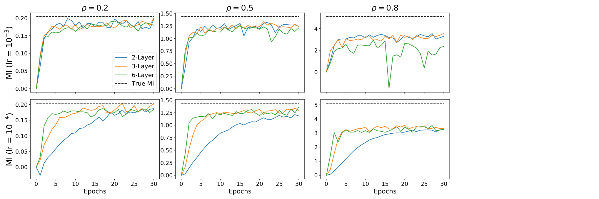
We further investigate how the neural network learning capacity affect MI estimation. In Figure S13 we compare the training dynamics of the FLO estimator with -layer neural networks, where and each hidden-layer has -units. A deeper network is generally considered to be more expressive. We see that using larger networks in general converge faster in terms of training iterations, and also obtain better MI estimates. However, more complex networks imply more computation per iteration, and it can be less stable when trained with larger learning rates.
F.6 Ablation study: Bi-linear critics and scaling
We setup the bi-linear critic experiment as follows. For the naive baseline FLO, we use the shared-network architecture for and , and use the in-batch shuffling to create the desired number of negative samples (FLO-shuff). For FLO-BiL, we adopt the following implementation: feature encoders are respectively modeled with three layer MLP with -unit hidden layers and ReLU activations, and we set the output dimension to . Then we concatenate the feature representation to and fed it to the network, which is a two-layer -unit MLP. Note that is merely a convenient modeling choice and can be further optimized for efficiency. Each epoch containing samples, and FLO-shuff is trained with fixed batch-size. For FLO-BiL, it is trained with batch-size set to the negative sample-size desired, because all in-batch data are served as negatives. We use the same learning rate for both cases, and this puts large-batch training at disadvantage, as fewer iterations are executed. To compensate for this, we use to set the total number of iterations for FLO-BiL, where are respectively the baseline training iteration and negative sample size used by FLO-shuff, and the number of negative sample K are . We are mostly interested in computation efficiency here so we do not compare the bound. In Figure S15, we see the cost for training FLO-shuff grows linearly as expected. For FLO-BiL, a U-shape cost curve is observed. This is because bilinear implementation has three networks total, while the shared MLP only have one network. This implies more computations when the batch size is small, however, as the batch size grows, the computation overhead is amortized by better parallelism employed with the bilinear strategy, thus increasing overall efficiency until the device capacity has been reached. This explains the initial drop in cost, followed by the anticipated square-root growth.
F.7 Comparison of learning dynamics for different variational MI bounds
In Figure S15, we show the learning dynamics of competing estimators for the 20-D Gaussian when . We can find FLO achieves the best accuracy, it also learns fast and stably. InfoNCE learns very stably, yet its learning efficiency varies significantly in small-batch and large-batch setups.

F.8 Comprehensive analyses of bias-variance trade-offs
To supplement our results in the main paper, here we provide additional bias-variance plots for different MI estimators under various settings. In Figure S16 we show the bias-variance plot of MI estimates for -D Gaussians. In this case, the network used are sufficiently comprehensive so sharp estimate is attainable. In all cases the estimation variance grows with MI value, which is consistent with the theoretical prediction that for tight estimators, the estimation variance grows exponential with MI [55]. In such cases, the argument for InfoNCE’s low-variance profile no longer holds: it is actually performing sub-optimally. For complex real applications, the negative sample size used might not provide an adequate estimate of ground-truth MI (i.e., the cap), and that is when InfoNCE’s low-variance profile actually helps. We also notice that, when the MI estimate is not exactly tight, but very close to the true value, the variance dropped considerably. This might provide alternative explanation (and opportunity) for the development near-optimal MI estimation theories, which is not covered in existing literature.

We also tried the single-sample estimators for NWJ, TUBA and FLO to their multi-sample InfoNCE-based counterparts (Figure S17), which is the comparison made by some of the prior studies (Note we do not apply Bilinear tric here, thus FLO seems similar to other methods). In this setting, the variance single-sample estimators’ variances are considerably larger, which explains their less favorable performance. Note that contradictory to theoretical predictions, a larger negative sample size does make NWJ, TUBA and FLO tighter empirically, although the gains are much lesser compare to that of InfoNCE (partly because these three estimators are already fairly tight relative to InfoNCE). This might be explained by a better optimization landscape due to reduced estimation variance. We conjecture that for multi-sample NWJ, TUBA and FLO, the performance in empirical applications such as self-supervised learning should be competitive to that of InfoNCE, which has never been reported in literature.

Appendix G Cross-view Representation Learning (Extended Analyses)
In addition to the results reported in the paper, we investigate how different latent dimension affect the results of the cross-view representation learning. We vary the latent dimension number from to , and plot label prediction accuracy for the corresponding latent representations in Figure S19. The same setup for the bi-linear experiment is used for the MI estimation (for all MI estimators), where the images are flattened to be fed to the MLPs. The representations are trained for epochs and the prediction model is trained for epochs. We also trained the model for another epochs and the conclusions are similar. We see that FDV works well for lower dimensions (e.g., ), and what works better for higher dimensions () are FLO and InfoNCE.
Appendix H Comparison with Classical MI Estimators
We also compare our FLO estimator to the classical MI estimators in Figure S19. The following implementations of baseline estimators for multi-dimensional data are considered: () KDE: we use kernel density estimators to approximate the joint and marginal likelihoods, then compute MI by definition; () NPEET 99 9 https://github.com/gregversteeg/NPEET, a variant of Kraskov’s -nearest neighbour (KNN) estimator [49, 80]; () KNNIE 1010 10 https://github.com/wgao9/knnie, the original KNN-estimator and its revised variant [28]. These models are tested on -D and -D Gaussians with varying strength of correlation, with their hyper-parameters tuned for best performance. Note that the notation of ‘‘best fit’’ is a little bit subjective, as we will fix the hyper-parameter for all dependency strength, and what works better for weak dependency might necessarily not work well for strong dependency. We choose the parameter whose result is visually most compelling. In addition to the above, we have also considered other estimators such as maximal-likelihood density ratio 1111 11 https://github.com/leomuckley/maximum-likelihood-mutual-information [73] and KNN with local non-uniformity correction 1212 12 https://github.com/BiuBiuBiLL/NPEET_LNC. However, these models either do not have a publicly available multi-dimensional implementation, or their codes do not produce reasonable results 1313 13 These are third-party python implementations, so BUGs are highly likely..
Appendix I Comparison to Parametric Variational Estimators and Bounds Targeting Alternative Information Metrics
Parametric variational estimators are typically associated with upper bound of MI [20, 65]. Inspired by multi-sample variational bounds for likelihood estimation, [16] derived a generic family of importance-weighted MI bounds that are provably tighter. These bounds usually require the additional knowledge of likelihood, and consequently they can not be directly used for data-driven MI estimations. On the other hand, these models do not suffer from the exponential scaling of variance suffered by non-parametric MI estimators. Note that MI is not the only measure to assess association between two random variables, some alternatives can potentially do better for specific applications. Examples include information [85], Rényi information [50], and the spectral information [36].
Appendix J Regression with Sensitive Attributes (Fair Learning) Experiments
J.1 Introduction to fair machine learning
Nowadays consequential decisions impacting people’s lives have been increasingly made by machine learning models. Such examples include loan approval, school admission, and advertising campaign, amongst others. While automated decision making has greatly simplified our lives, concerns have been raised on (inadvertently) echoing, even amplifying societal biases. Specially, algorithms are vulnerable in inheriting discrimination from the training data and passed on such prejudices in their predictions.
To address the growing need for mitigating algorithmic biases, research has been devoted in this direction under the name fair machine learning. While discrimination can take many definitions that are not necessarily compatible, in this study we focus on the most widely recognized criteria Demographic Parity (DP), as defined below
Definition J.1 (Demographic Parity, [22]).
The absolute difference between the selection rates of a decision rule of two demographic groups defined by sensitive attribute , i.e.,
| (S50) |
With multiple demographic groups, it is the maximal disparities between any two groups:
| (S51) |
J.2 Experiment details and analyses
To scrub the sensitive information from data, we consider the in-processing setup
| (S52) |
By regularizing model training with the violation of specified fairness metric , fairness is enforced during model training. In practice, people recognize that appealing to fairness sometimes cost the utility of an algorithm (e.g., prediction accuracy) [37]. So most applications seek to find their own sweet points on the fairness-utility curve. In our example, it is the DP-error curve. A fair-learning algorithm is consider good if it has lower error at the same level of DP control.
In this experiment, we compare our MI-based fair learning solutions to the state-of-the-art methods. Adversarial debiasing tries to maximize the prediction accuracy for while minimize the prediction accuracy for sensitivity group ID [87]. We use the implementation from AIF3601414 14 https://github.com/Trusted-AI/AIF360 package [13]. FERMI is a density-based estimator for the exponential Rényi mutual information , and we use the official codebase. For evaluation, we consider the adult data set from UCI data repository [7], which is the 1994 census data with k samples in the train set and k samples in the test set. The target task is to predict whether the income exceeds $50k, where gender is used as protected attribute. Note that we use this binary sensitive attribute data just to demonstrate our solution is competitive to existing solutions, where mostly developed for binary sensitive groups. Our solution can extend to more general settings where the sensitive attribute is continuous and high-dimensional.
We implement our fair regression model as follows. To embrace data uncertainty, we consider latent variable model , where are the observed predictor and labels. Under the variational inference framework [45], we write the as
| (S53) |
is modeled with standard Gaussian, and the approximate posterior is modeled by a neural network parameterizing the mean and variance of the latents (we use the standard mean-field approximation so cross-covariance is set to zero), and is a hyperparameter controlling the relative contribution of the KL term to the objective. Note that unlike in the standard ELBO we have dropped the term because we are not interested in modeling the covariates. Note this coincides with the variational information bottleneck (VIB) formulation [2]. Additionally, the posterior will not be conditioned on , but only on , because in practice, the labels are not available at inference time. All networks used here are standard three-layer MLP with hidden-units.
For Figure S20, we note that the adversarial de-biasing actually crashed in the DP range , so the results have to be removed. Since interpolation is used to connect different data points, it makes the adversarial scheme look good in this DP range, which is not the case. FERMI also gave unstable estimation in the DP range . Among the MI-based solutions, NWJ was most unstable. Performance-wise, InfoNCE, TUBA and FDV are mostly tied, with the latter two slightly better in the “more fair” solutions (i.e., at the low DP end).
Appendix K Self-supervised Learning
Our codebase is modified from a public PyTorch implementation1515 15 https://github.com/sthalles/SimCLR. Specifically, we train -dimensional feature representations by maximizing the self-MI between two random views of data, and report the test set classification accuracy using a linear classifier trained to convergence. We report performance based on ResNet-50, and some of the learning dynamics analyses are based on ResNet-18 for reasons of memory constraints. Hyper-parameters are adapted from the original SimCLR paper. For the large-batch scaling experiment, we first grid-search the best learning rate for the base batch-size, then grow the learning rate linearly with batch-size.
| Model | CCA | NWJ | TUBA | InfoNCE | FLO | FDV |
|---|---|---|---|---|---|---|
| Accuracy | 67.78 | 76.71 | 79.49 | 79.27 | 79.47 | 80.14 |
| NA | 5.73 | 4.78 | 4.65 | 4.84 | 4.67 |
Appendix L Bayesian Experimental Design
L.1 Noisy Linear Model
Our setup is the same as the Noisy Linear Model in [47]. We use 10 individual experimental designs. For encoder and encoder , we use MLP with 2-layer, 128-dim hidden layer, and set the feature dim as 512. We train models in 5000 epochs, the batch size is 64, and the learning rate is . Four MI estimators (NWJ, TUBA, InfoNCE, and FLO) has been compared in this experiment and we got four optimized designs. Then, we use MCMC to estimate the posterior of the parameters.
L.2 Pharmacokinetic Model
The settings of this experiment refer to the Pharmacokinetic Model of [47]. We use 10 individual experimental designs. The MLP is with 2-layer, 128-dim hidden layer, and set the output feature dim as 512. We train 10000 epochs with learning rate is via four methods (NWJ, TUBA, InfoNCE, FLO).
L.3 SIR Model
We here consider the spread of a disease within a population of N individuals, mod- elled by stochastic versions of the well-known SIR [4]. a susceptible state and can then move to an infectious state with an infection rate of . These infectious individuals then move to a recovered state with a recovery rate of , after which they can no longer be infected. The SIR model, governed by the state changes , thus has two model parameters .
The stochastic versions of these epidemiological processes are usually defined by a continuous-time Markov chain (CTMC), from which we can sample via the Gillespie algorithm [3]. However, this generally yields discrete population states that have undefined gradients. In order to test our gradient-based algorithm, we thus resort to an alternative simulation algorithm that uses stochastic differential equations (SDEs), where gradients can be approximated.
We first define population vectors for the SIR model and for the SEIR model. We can effectively ignore the population of recovered because the total population is fixed. The system of Itô SDEs for the above epidemiological processes is
| (S54) |
where is the drift term, is the diffusion term and is the Wiener process. Euler-Maruyama algorithm is used to simulate the sample paths of the above SDEs.
| (S55) |
We use the infection rate () as 0.1 and the recovery () rate as 0.01. The independent priors are N(0.1,0.02) and N(0.01, 0.002). The initial infection number is 10. We update MI one time after updating sampler three steps.We use RNN network with 2 layer 64 dim hidden layer construction to decoder the sequential design.
Appendix M Meta Learning
Intuitions. Now let us describe the new Meta-FLO model for meta-learning. Given a model space and a loss function , the true risk and the empirical risk of are respectively defined as and .Let us denote is the generalization error for the task distribution where all tasks originate, and is the empirical estimate. Our heuristic is simple, that is to optimize a tractable upper bound of the generalization risk given by
| (S56) |
For meta-learning, we sample -tasks for training and -tasks for testing, respectively denoted as and . We further decouple the learning algorithm into two parts: the meta-learner that consumes all train data to get the meta-model , and then task-adaptation learner which adapts the meta-model to the individual task data to get task model . For parameterized models such as deep nets, we denote as our meta parameters and as task-parameters, that is to say , , where can be understood as weights of deep nets. In subsequent discussions, we will also call the task-embedding. We can define the population meta-risk as , and similarly for the empirical risk evaluated on the query set . Our model is based on the following inequality [5]:
| (S57) |
which gives the main objective . We summarize our model architecture in Figure S21.
The sin-wave adaptation experiment involves regressing from the input () to the output of a sine wave , where amplitude and phase () of the sinusoid vary for each task. We use mean-squared error (MSE) as our loss and set the support-size = and query-size = . We use simple three-layer MLPs for all the models: regressor, prompt encoder, and FLO critics, with hidden units all set to . During training, we use an episode-size of . For MAML, we use the first-order implementation (FOMAML), and set inner learning rate to . For Meta-FLO, we set regularization strength to .