Yukawa vs. Newton: gravitational forces in a cubic cosmological simulation box
Abstract
We study the behaviour of Yukawa and Newtonian gravitational forces in a cubic box with fully periodic boundaries commonly encountered in N-body simulations of the structure formation. Placing a single gravitating body at the origin of coordinates, we reveal the scales at which non-negligible deviation from the Yukawa law occurs when the Newtonian approximation is employed. We discuss the results in terms of the corresponding physical distances today as well as earlier, back at the matter-dominated stage. Revisiting the problem for free boundaries, we also compare the periodic and plain gravitational forces for Yukawa-type interactions.
pacs
PACS-keydiscribing text of that key and PACS-keydiscribing text of that key1 Introduction
Nonlinear dynamics governing structure formation at sub-horizon scales is often modelled using the Newtonian approximation in cosmological simulations Gadget-4; Newton; 75. The absence of relativistic effects in the formulation is, however, a major drawback as they are an essential part of cosmological processes, and not to be neglected particularly in the era of precision cosmology. This can be overcome by employing the Yukawa gravitational potential instead of the Newtonian one in the equations of motion of the underlying N-body codes. The sought-for contribution of general relativistic effects is inherent in the Yukawa potential as it follows directly from the Einstein equations. The Yukawa-type interaction of gravitating bodies was initially introduced in Eingorn1 as the manifestation of gravitation at all scales, namely, at both sub- and super-horizon distances. Later, the associated time-dependent cutoff distance for the potential and force (i.e. the Yukawa interaction range, or the screening length) was revisited in EE where it was used (along with the cutoff scale from Hahn) to define the effective screening length which fully agrees with the sizes of the largest cosmic structures observed today. At small scales, well below , the Yukawa gravitational potential is reduced to its Newtonian counterpart. However, at scales comparable to the screening length and beyond those, two laws of gravity deviate from one another since unlike the Newtonian behaviour, the potential undergoes rapid exponential decay in the Yukawa formulation. In this connection, it is interesting to study the discrepancy in terms of the force generated by a single particle in a cubic box, conventionally utilized in N-body simulations. The results then can straightforwardly be translated into the physical setting to reveal the scales at which the Newtonian approximation differs significantly from the Yukawa law.
In the present work, our primary focus is on the comparison of Yukawa and Newtonian forces for a single gravitating body in a simulation box with three-dimensional periodic boundaries. We investigate how the behaviour of forces changes with increasing distance from the source and how it depends on the screening length of Yukawa gravity, i.e. what happens when the screening length is significantly smaller than, comparable to or larger than the box size. We then evaluate our results based on the corresponding physical distances, provided that the box size today is set to . Additionally, to see the impacts of periodicity on the force, we extend the analysis to include the problem with free boundaries.
The outline of this paper is as follows. In Section 2, we present the formulas for the Yukawa and Newtonian potentials and forces, both for free and periodic boundaries. The expressions for periodic boundaries are formulated via Ewald sums to ensure better correspondence with the available N-body simulations. We compare the behaviour of forces for various values of the screening length. In Section 3, we provide a more detailed analysis showing how far from the gravitating source the periodic Yukawa and Newtonian as well as the periodic and plain Yukawa forces begin to significantly differ from one another. We analyze the results in terms of the corresponding physical distances for a box size of today. In concluding Section 4 we provide a brief summary.
2 Potentials and forces
In the cosmological setting, the motivation for calculating the gravitational potential and force for periodic boundaries is twofold. From the theoretical point of view, it is possible that the universe is not simply connected, contrary to what is suggested by concordance cosmology, but multiply connected. Hence, as is a matter of investigation also in observational cosmology 49; 47; 48, the space may have toroidal topology: it may be shaped as a cubic torus (), the size of which is bounded from below by the available data 42. If this is the case, periodicity in three dimensions naturally requires that one should resort to fully periodic boundary conditions to accurately describe gravity at the scales of interest TTT. Nonetheless, if not imposed on physical grounds, i.e. when the study is based on concordance cosmology, periodic boundaries come into play in N-body codes for practical reasons. In order to mimic the interactions in the infinite universe, simulations are generally run for cubic boxes replicated periodically in three dimensions Gadget-4; Newton; 75; 77.
Cosmological N-body simulations based on the Newtonian approximation often employ the Ewald method so that the very slowly converging series in the periodic force expression becomes numerically manageable Hernquist; Klessen. Though the Yukawa force has good convergence properties, especially for the small values of the interaction range in comparison to the box size TTT, we employ the Ewald summations for both laws to ensure consistency.
Below we present, respectively, the formulas for the rescaled Yukawa-Ewald gravitational potential and -component of the corresponding rescaled gravitational force in a cubic simulation box TTT. They are sourced by a single particle of mass at the origin of comoving Cartesian coordinates as well as its periodic images which are positioned at , , where represents the cubic torus period:
| (2.1) | |||||
| (2.2) | |||||
where ,
and
The rescaled quantities (with tildes) in the above expressions as well as throughout the paper follow from the definitions
| (2.5) |
where is the scale factor. As regards the rescaled potential , if we multiply it by (where is the Newtonian gravitational constant and is the speed of light), and then sum up such contributions from all N particles in the simulation box, adding also the term , then we get the total scalar metric perturbation TTT.
In an identical setup, the rescaled Newton-Ewald potential and -component of the gravitational force read Hernquist; Klessen
| (2.6) | |||||
| (2.7) | |||||
In both expressions (2.2) and (2.7), the free parameter of the Ewald formulation is set to , according to Hernquist; Klessen, to achieve good accuracy at fairly low computational cost. In principle, the results do not depend on the choice of for a reasonable range of values. Assigned an optimal value, it rather serves to facilitate rapid convergence of the series so that adequate precision may be reached by including a small number of terms in the summation, which reduces computational effort.
Given the possibility that periodicity may not be demanded by topology, and hence the related effects in simulations may be artificial 2006.10399, we find it worthwhile to study two laws of gravity also for free boundaries. Losing the lattice, we formulate the solutions again for a single gravitating body, placed at . The rescaled Yukawa potential and -component of the gravitational force are then, respectively,
| (2.8) |
| (2.9) |
whereas the rescaled Newtonian potential and -component of the gravitational force are
| (2.10) |
| (2.11) |
In Figs. 1(a) - 2(b), we simultaneously plot four force curves, according to (2.2), (2.7), (2.9) and (2.11), versus (in the case of fixed ) for , respectively. We aim to demonstrate how they behave with increasing distance from the gravitating body, depending on the effective screening length , especially when periodic boundaries are imposed.

Looking first at Figs. 1(a) and 1(b), one realizes that the curves corresponding to two different laws of gravity are visibly separated from one another except in the immediate vicinity of the source placed at , and near , where the Yukawa-Ewald and Newton-Ewald forces tend to zero. The Ewald summations of Yukawa and Newtonian forces do not deviate much from the corresponding plain (Yukawa and Newtonian) forces themselves which, unlike the Ewald summations, do not involve the effects of periodicity. Contrarily, in Figs. 2(a) and 2(b), the plain Yukawa and Newtonian forces remain close to each other just like the curves demonstrating the corresponding Ewald forces, and now these two sets are separated within the range of interest instead. The reason for such an outcome is the following: for small , the difference in the forms of gravitational interaction for Yukawa and Newtonian laws comes into play at rather small distances from the source due to the small range of the exponentially decaying Yukawa force, characterized by nothing but the interaction range . The Ewald summation here does not significantly change the behaviour of the plain Yukawa force, again, because of the smallness of the interaction range, which is well below the half-box size. For larger , however, periodicity does make a difference and one sees that Ewald forces decrease rapidly to reach zero at in the last two figures. Nevertheless, the Yukawa vs. Newtonian behaviour of gravity is no longer recognizable, as the interaction range is equal to or larger than the box size in Figs. 2(a) and 2(b), respectively.

3 Deviations from the plain Yukawa and Yukawa-Ewald forces
Elaborating further on our analysis in the previous section, we now zoom into the region in the box where deviations from the Yukawa-Ewald and plain Yukawa forces become non-negligible. To begin with, we employ the formulas (2.2) and (2.7) and plot the relative error (for ) against , i.e. the distance from the source particle. In Fig. 3(a), we show that for , the distinction among periodic forces grows very fast. A relative error as large as takes place at , and the error is encountered at a distance smaller than of the box size, that is at . Since the difference between Yukawa-Ewald and Newton-Ewald forces is sensitive to the screening length, when we fix in Fig. 3(b), we observe the and errors at the points and , respectively, that are shifted further from the previous two towards the middle of the box edge. Owing to the larger cutoff scale of the Yukawa force here, two laws of gravity behave similarly throughout a larger region surrounding the gravitating body; yet both computed distances are still significantly small relative to the box size, as merely equals one tenth of it.
Then, using the formulas (2.2) and (2.9) (again, calculated for ), we plot the relative error versus in Fig. 4. We consider two cases with to study where in the box the plain Yukawa and Yukawa-Ewald forces begin to significantly deviate from one another. This time, for both curves the and errors occur at and , respectively, and we see that locations of two fixed percent errors shift towards the point with increasing . As mentioned previously, periodic boundaries result in deviations from the plain Yukawa force, especially when the cutoff distance exceeds the half-box size, because at the Yukawa-Ewald force tends to zero regardless of the greater interaction range. For the same reason, deviations take place closer to the center of the edge rather than to the gravitating source.


It is worth noting at this point that as we consider a sample simulation box in the following steps, the range of interest for will be , which corresponds to a period between redshifts and for our particular example.
In Fig. 5(a), four distinct percent error values ranging from to for Ewald forces are displayed with respect to where they are encountered in the simulation box for different . The physical size of the box is set to today (), i.e. . This approximately corresponds to on the horizontal axis via , where is determined from Eq. (41) of EE,
| (3.12) |
using the current values of the cosmological parameters relevant to the calculation of , the Hubble parameter, as reported in Planck. The same relation indicates that the minimum value of on the plot () corresponds to the redshift . The physical distances at which the fixed percent errors are encountered at the present time approximately equal 530 (), 122 (), 37 () and 12 () . We see clearly in this figure that the distances of relative error points from the source are generally much smaller than the box size. Fig. 5(b) demonstrates the same four fixed percent error curves in an identical setting, except now for the relative error associated with the Yukawa-Ewald and plain Yukawa forces. Herein the respective physical distances at the present time approximately equal 173 (), 82 (), 38 () and 18 () . Unlike the behaviour in the previous figure, locations of percent errors shift towards the middle of the box edge as we move towards larger redshifts (smaller ).
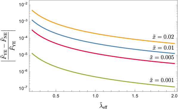
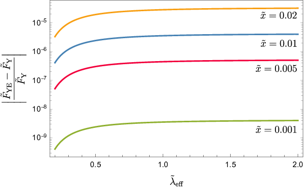
As an alternative representation, in Figs. 6(a) and 6(b) we present, respectively, the relative error for the Yukawa-Ewald vs. Newton-Ewald forces and Yukawa-Ewald vs. plain Yukawa forces for the range at certain fixed points in the box that correspond to and distances from the gravitating source today.
4 Conclusion
In the present work we have provided a thorough comparison of the Yukawa and Newtonian gravitational forces that are generated by a particle in a cubic box with periodic boundaries. As is the conventional method in cosmological N-body simulations, we have employed Ewald sums in expressing both periodic forces. We have additionally investigated how the Yukawa-Ewald force compares to the plain Yukawa force of the free boundary problem to reveal the effects of periodicity for Yukawa-type interactions.
With a detailed analysis, we have shown that regarding the Yukawa-Ewald and Newton-Ewald forces, a relative error of already takes place at 12 Mpc from the gravitating source, followed by an error of at 37 Mpc distance today, while and . As for the plain Yukawa vs. Yukawa-Ewald forces, the corresponding distances are revealed to be 18 and 38 Mpc, respectively. The measure of discrepancy between the plain Newtonian and periodic Newton-Ewald forces has previously been studied in view of cosmological simulations Gadget-4; 2006.10399, with a reported relative error of produced at distances as small as of the box size Gadget-4. Here we have shown that the error associated with different laws of gravitation, i.e. the difference between the Yukawa-Ewald and Newton-Ewald forces is more significant since the error is already encountered at a point closer to the source than . At earlier epochs, for smaller and , the error points are shifted towards the gravitating body. Therefore, in simulations that employ periodic Newtonian forces, non-negligible deviations from the periodic Yukawa force are expected, especially throughout the matter-dominated epoch that is directly associated with structure formation. Meanwhile, imposing periodic boundaries also results in deviations from the plain Yukawa force, but the error associated with periodicity in Yukawa-type interactions is less significant (as it clearly follows from the comparison of Figs. 6(a) and 6(b)).
Finally, we would like to comment on the larger percent errors (see, for instance, the orange curve in Fig. 5(a)) encountered with increasing distance from the source. In our analysis, we have considered a single gravitating body and naturally, the gravitational force due to this particle is decreasing with distance. Though the calculated error is growing significantly as we move further away from the source, it is of no importance at large enough scales because had there been other gravitating bodies included in the configuration, as is the case in the physical setting, the forces induced by neighboring particles in that location would be much larger than the force due to the original source and the latter would eventually become negligible. In this connection, the errors associated with the single particle case in this study are not to be considered relevant to the multi-particle configurations at significantly large scales.
Declarations
Authors’ Contributions: Conceptualization: ME; Methodology: EC and ME; Formal analysis and investigation: EC and ME; Writing - review and editing: EC and ME; Visualization: EC; Supervision: ME; Project administration: ME; Funding acquisition: ME; Writing - original draft preparation: EC.
Funding: The work of Maxim Eingorn was supported by National Science Foundation (HRD Award #1954454).
Availability of data: All data generated or analyzed in the study are included in the article.
Conflicts of interest: The authors have no conflicts of interest to declare that are relevant to the content of this
article.
References
- (1) V. Springel, R. Pakmor, O. Zier and M. Reinecke, Simulating cosmic structure formation with the GADGET-4 code. MNRAS 506, (2021) 2871. arXiv:2010.03567 [astro-ph.IM]
- (2) K. Dolag, S. Borgani, S. Schindler, A. Diaferio and A.M. Bykov, Simulation techniques for cosmological simulations. SSRv 134, (2008) 229. arXiv:0801.1023 [astro-ph]
- (3) J.S. Bagla, Cosmological N-body simulation: techniques, scope and status. Curr. Sci. 88, (2005) 1088. arXiv:astro-ph/0411043
- (4) M. Eingorn, First-order cosmological perturbations engendered by point-like masses. ApJ 825, (2016) 84. arXiv:1509.03835 [gr-qc]
- (5) E. Canay, M. Eingorn, Duel of cosmological screening lengths. Phys. Dark Univ. 29, (2020) 100565. arXiv:2002.00437 [gr-qc]
- (6) O. Hahn, A. Paranjape, General relativistic screening in cosmological simulations. Phys. Rev. D 94, (2016) 083511. arXiv:1602.07699 [astro-ph.CO]
- (7) G. Aslanyan, A.V. Manohar, Constraints on the global topology and size of the universe from the cosmic microwave background. JCAP 06, (2012) 003. arXiv:1104.0015 [astro-ph.CO]
- (8) P. Bielewicz, A.J. Banday, Constraints on the topology of the Universe derived from the 7-year WMAP data. MNRAS 412, (2011) 2104. arXiv:1012.3549 [astro-ph.CO]
- (9) P. Bielewicz, A.J. Banday, K.M. Gorski, Constraints on the topology of the Universe derived from the 7-year WMAP CMB data and prospects of constraining the topology using CMB polarisation maps. Proceedings of the XLVIIth Rencontres de Moriond, eds. E. Auge, J. Dumarchez and J. Tran Thanh Van (ARISF, Paris, 2012). arXiv:1303.4004 [astro-ph.CO]
- (10) P.A.R. Ade et al. [Planck Collaboration], Planck 2015 results. XVIII. Background geometry and topology. A&A 594, (2016) A18. arXiv:1502.01593 [astro-ph.CO]
- (11) M. Eingorn, E. Canay, J.M. Metcalf, M. Brilenkov and A. Zhuk, Effect of the cubic torus topology on cosmological perturbations. Universe 7, (2021) 469. arXiv:2106.14004 [gr-qc]
- (12) B. Marcos, T. Baertschiger, M. Joyce, A. Gabrielli and F.S. Labini, Linear perturbative theory of the discrete cosmological N-body problem. Phys. Rev. D 73, (2006) 103507. arXiv:astro-ph/0601479
- (13) R. Klessen, GRAPESPH with fully periodic boundary conditions: fragmentation of molecular clouds. MNRAS 292, (1997) 11. arXiv:astro-ph/9704004
- (14) L. Hernquist, F.R. Bouchet and Y. Suto, Application of the Ewald Method to Cosmological N-Body Simulations. ApJS 75, (1991) 231.
- (15) G. Rácz, I. Szapudi, I. Csabai, L. Dobos, The anisotropy of the power spectrum in periodic cosmological simulations. MNRAS 503, (2021) 5638. arXiv:2006.10399 [astro-ph.CO]
- (16) N. Aghanim et al. [Planck Collaboration], Planck 2018 results. VI. Cosmological parameters. A&A 641, (2020) A6. arXiv:1807.06209 [astro-ph.CO]