Online Multi-Agent Forecasting with Interpretable Collaborative Graph Neural Networks
Abstract
This paper considers predicting future statuses of multiple agents in an online fashion by exploiting dynamic interactions in the system. We propose a novel collaborative prediction unit (CoPU), which aggregates the predictions from multiple collaborative predictors according to a collaborative graph. Each collaborative predictor is trained to predict the status of an agent by considering the impact of another agent. The edge weights of the collaborative graph reflect the importance of each predictor. The collaborative graph is adjusted online by multiplicative update, which can be motivated by minimizing an explicit objective. With this objective, we also conduct regret analysis to indicate that, along with training, our CoPU achieves similar performance with the best individual collaborative predictor in hindsight. This theoretical interpretability distinguishes our method from many other graph networks. To progressively refine predictions, multiple CoPUs are stacked to form a collaborative graph neural network. Extensive experiments are conducted on three tasks: online simulated trajectory prediction, online human motion prediction and online traffic speed prediction, and our methods outperform state-of-the-art works on the three tasks by , and on average, respectively.
Index Terms:
Online multi-agent forecasting, collaborative graph, collaborative predictor, theoretical regret analysisI Introduction
Dynamic multi-agent systems depict a group of co-evolving agents which perform interactions to activate or constrain the pattern of each other. Dynamic systems are ubiquitous and critical in many real-world scenarios, such as transportation networks and smart grids [1, 2, 3]. In many applications, we need to predict future measurements of a multi-agent system, such as the traffic on various roads within hours for route planning [4].
To forecast the future status of systems, previous works usually train models with finite training datasets and evaluate models with unseen test sets in offline settings. The offline models essentially assume the training and test samples are stationary and share the same distribution, thus fixed models could generalize to arbitrary systemic states [5, 6, 7]. We sketch the offline learning paradigms in Fig. 1 (a).

However, limited training sets are still hard to depict complicated real-world scenarios [8], and the multi-agent system could be highly dynamic, resulting in the infinitely possible states changing over time. To make reliable predictions for the dynamic multi-agent system with streaming states, we need an online model to adapt to a potential varying environment in real-time. Taking streaming data captured along time as inputs, the online multi-agent forecasting model is tested and trained simultaneously step-by-step and never stops. The online learning methods never fix the model parameters, while they always tune the models to capture the dynamic even infinite systemic states along with iteration. The online learning paradigm is sketched in Fig. 1 (b).
Moreover, to learn the pattern of multiple agents, previous methods usually regard every single agent in an isolated manner, such as autoregressive models [9], hidden Markov models [10], Kalman filter [11], and deep sequence-to-sequence models [12], which exhibit increasingly powerful modeling; however, for multi-agent forecasting, these methods might underestimate potential interactions among the co-evolving agents in a dynamic system. For example, traffic flows on neighboring streets are mutually dependent; and human body-parts might constrain each other during moving. To leverage such relations, some works build graphs to model the relations for representation learning [13]. For example, in traffic analysis, [14] builds a road network according to the urban traffic map. To capture more flexible relations, some works build trainable graphs as model parameters, whose edge weights are updated in an end-to-end setting [15, 16]. However, such graphs are typically constructed through trials and errors, lacking direct guidance and theoretical interpretation, leading to the difficulties of rigorous understanding and reasonable improvement. In this work, we propose interpretable update steps to learn a graph that captures the collaboration among agents. We further provide the theoretical justification of this graph.
This work aims to design an online forecasting model, which captures the dynamic interactions among agents for real-time prediction. The core component of our method is a collaborative prediction unit (CoPU), which automatically builds a trainable collaborative graph to represent the systematic interactions. This collaborative graph includes two types of nodes: agents and collaborative pairs. A collaborative pair, essentially formed by a pair of agents, refers to the mutual collaboration between the two agents. Fed with collaborative pairs, a collaborative predictor is built in CoPU to forecast each agent’s status, aiming to leverage the inter-agent impacts, thus the collaborative predictors produce the possible measurements for each agent according to the effects from another agent. Finally, we learn a weight on each edge of the collaborative graph, aggregating all collaborative predictors for the final predictions. The trainable edge weights reflect the influence level of each collaborative pair. Notably, in CoPU, the collaborative predictor is parameterized and trained through online gradient descent, while, in a different way, the edge weights are adjusted by an online multiplicative update step-by-step to reflect the dynamic topology. The update strategy can be motivated by solving an explicit objective function. To understand CoPU, we conduct regret analysis and prove that the performance of CoPU can converge to that of the best single collaborative predictor.
One advantage of the proposed method is its interpretability, which comes from three aspects. 1) Algorithm: the edge weights of our collaborative graph are obtained by solving an explicit optimization, while previous works are based on heuristic designs [5, 17, 18, 19, 20, 13]. 2) Theory: we prove that the gap between the predictions based on our collaborative graph and the optimal collaborative pair is within a bounded range. In other words, our collaborative graph describes the information and importance carried by different collaborative pairs for prediction. In comparison, previous works have no theoretical support at all. 3) Visualization: our interpretability is reflected based on human understanding. In experiments, we visualize the learned collaborative graphs changing over time, reflecting comprehensible, reasonable and dynamic graphs in the online setting.
To produce more precise predictions, we further stack a series of CoPUs to build a collaborative graph neural network (CoGNN), progressively refining the predictions. In CoGNN, each CoPU with a collaborative graph is directly supervised by the ground-truth targets, thus all CoPUs predict agents’ statuses in the original measurement space. Skip-connections across CoPUs are leveraged to stablize prediction. Compared to many spatio-temporal graph neural networks [17, 21, 14], the advantages of CoGNN include its interpretability and simplicity, because the information aggregation is performed according to the importance of collaborative pairs in the clear output space, while previous methods generate graph features in the hidden space.
We conduct extensive experiments to validate the proposed CoGNNs on three important tasks: online simulated trajectory prediction, online human motion prediction and online traffic speed prediction. We note that we formulate a new online setup that simultaneously trains and tests models, and we adapt previous offline state-of-the-art methods to the online setting. According to the results, CoGNNs significantly outperform state-of-the-art methods.
The main contributions are as follows.
- •
We propose a novel collaborative prediction unit (CoPU), which predicts the future statuses of multiple correlated agents based on a collaborative graph. The collaborative graph contains two types of nodes; that is, individual agents and collaborative pairs, which represent the agent dynamics and collaboration status between agents. In this way, an agent could share customized information with each neighboring agent via the collaborative pair.
- •
We employ an online multiplicatively update algorithm to learn the edge weights of the collaborative graph on the fly to solve an explicit objective function; see Eq. (7). In this way, the graph tuned and tested simultaneously in an online setting effectively adapts to the changing states of the dynamic data flows. Moreover, the collaborative graph can be theoretically justified through regret analysis.
- •
We propose a novel collaborative graph neural network (CoGNN), which consists of a sequence of CoPUs and progressively refines multi-agent forecasting.
- •
We conduct extensive experiments to validate the effectiveness, interpretation and convergence of our method, which obtains superior and reasonable results.
The rest of this paper is organized as follows. In section II, we introduce some works related to multi-agent forecasting, graph deep learning and online learning for prediction. In section III, we define and formulate the problem. In section IV, we construct the proposed CoPU, introduce the online training method, and conduct the theoretical regret analysis. In section V, we construct the entire CoGNN model. Finally, the experiments validating the advantages of our model and the conclusion of the paper are provided in Section VI and Section VII.
II Related Works
In this section, we introduce critical methods related to our works from aspects of 1) multi-agent time-series forecasting, 2) graph deep learning and 3) online learning for prediction.
Multi-agent forecasting of time-series. Multi-agent forecasting has attracted huge attention and brought wide applications. In the early era, state models were studied [22, 10, 23, 24]. Recently, data-driven models extract deep representations. DeepState [25], Res-sup. [26], AGED [27] and LSTNet [28] design recurrent networks for stability. TCN [29] proposes feed-forward convolution for temporal dependencies. However, the methods do not consider the informative interactions among agents to benefit forecasting.
Recently, some works construct graphs to explicitly exploit the agent relations. NRI [5] infers graphs via an autoencoder for prediction. S-RNN [30] builds factor graphs to propagate agents’ information. DCRNN [18] and ST-GCN [14] incorporate distance-based graphs for traffic forecasting. GraphWaveNet [31] and Traj-GCN [15] use adaptive topologies to capture potential dependencies. DMGNN [17] builds multiscale graphs. However, most graphs are built with limited human priors or designed through trials and errors, lacking theoretical guarantees and interpretation. In this work, we develop a novel framework for multi-agent forecasting, which infers a collaborative graph with theoretical justification.
Graph deep learning. The expressiveness of graphs contributes to various scenarios such as social networks [32], bioinformatics networks [33] and human behaviors [19, 20]. Graph neural networks (GNNs) [34, 35, 36, 37], which expand deep leading to the non-Euclidean domain, have attracted explosive interests. GNNs can be mainly categorized into the spectral-domain-based [38, 39, 34] and vertex-domain-based [40, 41, 35, 42, 43, 44, 45], which respectively learn the patterns from the graph Fourier representations or the raw topologies. In this work, we learn interpretable graphs for multi-agent forecasting, which captures dynamic and complex correlations for precise prediction.
Online learning for prediction. A dynamic system evolves with potentially infinite states over time, performing on online streaming data [46]. Tailored for the data flows, online prediction models have been designed to update in real-time [47]. Traditional kernel-based works develop budgeted kernel learning [48, 49, 50, 51], RF approximations [52, 53, 54] and multi-kernel learning methods [55]. Recently, some deep-learning-based methods are proposed for online prediction [56, 57, 58], whose network structures are specifically designed. In this work, we train graph-based multi-agent forecasting models in an online setting, and optimize graphs to depict the agents’ interactions in real-time.
III Problem Formulation
With the time-series measurements collected by multiple agents in real-time, the task of online multi-agent forecasting essentially aims to predict the future statuses of each agent at each online time stamp based on the corresponding historical states. Mathematically, for the th agent , at time stamp , let be the measurements of the observed clip with length and feature dimension , recording ’s states within time interval ; and be the measurements of the corresponding ground-truth clip in the future, reflecting ’s states within . We note that the length of historical and future sequences could be different, while we here use to simplify notation. Our online predictor aims to produce
to approximate the ground-truth , where the input data is captured from streaming data flow at time stamp . Note that the model indexed by is updated online. The online setting is crucial because the online predictor can effectively adapt to the unseen, or highly dynamic data distribution.
In contrast, previous works [5, 20, 15, 16, 59] mostly consider an offline setting, which includes training and testing phases. In the training phase, a predictor is optimized based on a training dataset; in the testing phase, the predictor is fixed and deployed on a testing dataset. Mathematically, let be an offline predictor, be the training dataset and be the testing dataset, the training and testing phases work as
These offline methods assume the training and testing time-series should share the same data distribution and the resulting offline predictors would be hardly adapt to domain shift in the testing phase.
To design an online predictor, our core strategy is to exploit the dynamic mutual relations of agents and capture their evolution status through online learning. To model pairwise collaborations, we introduce a key concept, collaborative pair, which groups two agents and can be used to reflect the effect from one agent to another in a multi-agent system. For example, the th agent and the th agent form a collaborative pair to indicate the directed effect from to . In this way, to predict the future status of the th agent, we consider , which exploits information from all the collaborative pairs of to benefit its prediction. This model considers each collaborative pair as a basic element, which is different from previous works that regard each individual agent as a basic element [15, 16].
IV Collaborative Prediction Unit
To develop an online multi-agent forecasting model, we propose a collaborative prediction unit (CoPU) as a basic module, which predicts the status of each agent from associated collaborative pairs via an collaborative graph.
IV-A Collaborative graph
To exploit the interactions among agents, we propose a collaborative graph that explicitly models the pairwise correlations. Let be a collaborative graph, where is the agent set with modeling the th agent, is the set of collaborative pairs with modeling the th collaborative pair; and is the collaborative graph adjacency matrix trained online, whose th element reflects the influence level from to at time stamp . Note that this collaborative graph is asymmetric and dynamic; that is, each collaborative edge represents a directional relationship between agents and each collaborative edge weight is time-varying during the online training process.

Different from many ordinary graphs, the collaborative graph has two types of nodes: agent and collaborative pair. Agents are actual nodes; while collaborative pairs are virtual nodes as they are naturally obtained when agents are given, which have directions. To predict the future status of each agent, we rely on each of its associated collaborative pairs to produce a possible future status for such an agent; and then, the final status is obtained by averaging all the possible statuses based on the weighted collaborative edges.
Different from many previous graph-convolution-based and message-passing-based models [15, 16, 59, 5, 6, 7], where each node shares the same node feature to all of its neighbors without considering the demand of each one of its neighbors, our model, based on a collaborative pair, helps the prediction of by sharing customized information according to ’s status.
IV-B Model design
Based on the collaborative graph, to construct the CoPU, we consider two key operations in series: collaborative-pair-based prediction, which predicts an agent’s future status based on an associated collaborative pair, which generate all possible predictions with the collaborative effects between agents, and weighted collaborative-graph-based aggregation, which obtains the final prediction. Fig. 2 illustrates the CoPU, where the left plot shows the modeling thoughts, and the right plot shows the detailed computation.
Collaborative-pair-based prediction. To explicitly form a collaborative pair, which represent the collaborative states of two agent in history, we propose a combination function to directedly combine the measurements of two agents. Given the observed measurements , , the state of the collaborative pair is
| (1) |
The collaborative state carries the directed effects from the agent to the agent .
Based on the collaborative pairs and their states, we propose a collaborative predictor, which embeds any collaborative pair to predict an agent’s future status under the corresponding effects. Let the collaborative predictor be , where is the parameter trained online at time . To predict under the collaborative effects from , the predicted status is
| (2) |
The physical meaning of is one possible future trajectory for by considering the influence from .
For a collaborative pair, the aggregation function and the predictor could be designed in numerous forms. Here we specifically consider three typical forms:
- •
Autoregressive model. Let concatenate the multi-order differences of two agents, i.e., , which provides a polynomial distance feature. We then vectorize by reshaping it along time, and directly set a linear to learn .
- •
LSTM model. Let concatenate the measurements of the two agents, i.e., . The concatenation of the raw measurements reduces the dimensions and encourages more flexible information. We employ a one-layer LSTM as on to extract the temporal dynamics.
- •
Temporal convolution model. We also consider as the raw measurement concatenation. We then perform two layers of 1-D convolution along time to capture sequential dynamics. A function is used as the activation after the first convolution to enhance flexibility.
Each agent has collaborative pairs, so we predict possible future statuses for one agent. To obtain the final prediction, we need to adaptively aggregate the possibilities.
Collaborative-graph-based aggregation. Given the possible future status for an agent, which is predicted based on each associated collaborative pair, we aggregate these statuses with different weights on the edge of the collaborative graph, where the edge weights are updated online and reflect the influence level from one agent to another. Mathematically, let the graph adjacency matrix at iteration step be , whose the th element is . The final prediction of under the effects from all the associated collaborative pairs is formulated as
| (3) |
where the edge weights are normalized for any agent . In all, the feed-forward operations of the CoPU is formulated as
| (4) |
where denotes the normalized collaborative edge weights.
Compared to most common graph-based models, which bridge the same types of nodes with a scalar edge weight, the proposed CoPU considers the heterogeneous nodes of agents and collaborative pairs, carrying individual dynamics the interactive effects in a hybrid manner. The CoPU essentially aggregates the comprehensive information from the collaborative pairs with different importance. Moreover, the proposed CoPU has a similar framework with the online expert mixture algorithm [60, 55], as the different collaborative predictors associated with an agent could be regarded as experts; however, each collaborative predictor explicitly exploits the customized information for the associated agent based on the corresponding collaborative pair, instead of producing an untargeted prediction independently like most expert mixture methods.
IV-C Optimization
CoPU enables a complete multi-agent forecasting pipeline, and the internal parameters could be trained given the prediction targets. To train the CoPU online, at each iteration , we update the model parameters to minimize the loss function:
| (5) |
where denotes a fixed and convex loss function evaluated at time ; is the length of iterations before the current stamp. Since is a convex function (e.g., loss) w.r.t. , we consider an upper bound of it,
| (6) |
To minimize Eq. (6), instead of using common online gradient descent to update and together, we consider different updating mechanisms, which bring theoretical guarantees. We separately optimize the parameters and with different steps. First, at time , the parameter could be trained by online gradient decent; that is,
where we use to simplify ; is the learning rate. Next, for , we employ a multiplicative exponentiated update, which is inspired from the randomized weighted majority of online learning [60]. We assume the optimal edge weight to be , and is updated through
| (7) | ||||
where denotes the KL-divergence between the optimized and the collaborative weight at the last iteration step. The optimization ensures the continuity and smoothness of the collaborative graph structure by minimizing the element-wise distances and distribution divergence. We also normalize the new collaborative edge weights by .
In previous graph neural networks [17, 21, 15, 16], graphs are obtained through either heuristic designs or end-to-end learning in a black-box, which lack a clear objective and theoretical justification. Compared to these works, the proposed method obtains the edge weights of the collaborative graph through optimizing an explicit objective function (7), which could be derived as an update function based on the input features and historical states in an online setting.
IV-D Comparison with previous works
The proposed CoPU is seemingly similar to spatio-temporal-graph convolution operations [17, 21, 14] and neural-message-passing operations [5, 6, 7]. Here we clarify the differences;
Compared to spatio-temporal-graph convolution operations [17, 21, 14], the proposed CoPU is novel from three aspects:
- •
Interpretable graph learning. Previous models usually build non-grid structures by using predefined graphs or adjusting the graph in an intractable black-box. Each CoPU contains an interpretable graph that optimizes an explicit objective function for model training and has a theoretical implication.
- •
Customized feature propagation. Previous works consider each node shares the same feature to all of its neighbors without considering the demands of neighbors. In CoPU, a node shares a customized feature to each neighbor via the collaborative pairs.
- •
Interpretable output. Previous methods build deep graph networks to learn the agent’s dynamics in the hidden high-dimensional spaces, lacking the interpretation of feature representation; while each CoPU predicts agents’ future statuses, which lie in the original measurement space.
Previous neural-message-passing-based works [5, 6, 7] include two steps to propagate information: v2e, which transforms the information of a pair of nodes to an edge, and e2v, which aggregates the information of edges to a node. Compared to those methods, the proposed CoPU is novel from three aspects:
- •
Interpretable graph learning. Previous works either build predefined graphs based on physical constraints or learn graph structures with errors and trials in black-boxes; while the edge weights of our collaborative graph are obtained by optimizing an explicit objective function and has theoretical justification.
- •
Meaning of v2e. In the v2e step, previous works update the embedding of each edge, which is an intermediate-feature-level fusion; while our CoPU directly generates the prediction of a node conditioned on another node, which is an output-level fusion.
- •
Meaning of e2v. In the e2v step, previous works consider the mean aggregation, which assigns the same weight for each one of the neighbors; while our CoPU adopts the weighted aggregation, where the weights are the edge weights in the collaborative graph, obtained through multiplicative updating.
IV-E Theoretical interpretation
To understand CoPU, we conduct regret analysis. We consider the best single collaborative predictor as our regret baseline and analyze the gap from our CoPU to this predictor. The best predictor has a straightforward meaning and its corresponding collaborative pair makes the most significant effect in predicting an agent’s future status. We aim to demonstrate that the regret tends to be finite in the online setting, which indicates the properties of our CoPU and the training algorithm from two aspects:
- •
The CoPU trained online could converge to a statistically stable state during the training process.
- •
The performance of CoPU achieves a limited gap from the best single collaborative pair in statistics, reflecting that CoPU captures significant and reasonable collaborations for effective and interpretable prediction.
Here we define the collaborative pair in the best collaborative predictor. For the th agent, it has collaborative pairs, . The collaborative pair for in the best collaborative predictor is obtained via
| (8) |
where denotes the parameters of the best collaborative predictor at iteration step . However, it is hard to implement an online model by directly determining and meanwhile optimizing ; that is why CoPU builds a collaborative graph with trainable weights to achieve a soft collaborative mechanism; see Eq.(4).
To measure the performance gap between the best collaborative predictor and CoPU, we define the static regret based on the difference between the accumulated loss of CoPU and that of the best collaborative predictor in hindsight,
where we simplify as . The regret reflects the gap between the CoPU and the best collaborative predictor, as well as the convergence rate of online learning.
To study the CoPU and the performance gap, we aim to calculate an upper bound of the regret. To facilitate the closed-form theoretical analysis, we consider a basic predictor (a linear autoregressive model) and propose the following assumptions that are commonly satisfied by our model:
(AS1) For the collaborative predictor at time , , given any collaborative pair, the loss is convex w.r.t. .
(AS2) For any bounded , where , and any collaborative pair, we have a bounded loss, , and a bounded gradient, .
Then, we propose two lemmas, which help to derive the upper bounds of regret. We first analyze the loss gap between arbitrary collaborative predictors and the best collaborative predictor.
Lemma 1.
Let and be the predictions of the best collaborative predictor and arbitrary one. Under AS1 and AS2, for any collaborative pair , we have
where is the learning rate; is the upper bound of the norm of parameters; and is the Lipschitz constant.
Proof.
Given any determined parameter of the collaborative predictor, for any collaborative pair , we have
| (9) |
Considering the convexity property of the loss function (see AS1), the gradient of the loss function satisfies
| (10) |
Plugging Inequality (10) into Eq. (9), we could easily obtain the following inequality by rearranging some terms,
| (11) | ||||
We further consider the assumption AS2 that points out the upper bound of and the Lipschitz constant of the gradient ; that is, for any collaborative predictor, we have and . We then summing Inequality (11) over , we could easily derive
| (12) |
where we assume the initial parameter to have a very small value, leading to , and consider to be non-negative.
Additionally, we divide by the number of iterations at the both side of Inequality (12) to complete the proof.
| (13) |
∎
Note that Lemma 1 are hold for any collaborative pair, so that, in hindsight, we could choose to be the parameter at iteration step and use the predicted status , which is output from the collaborative predictor corresponding to the single optimal collaborative pair .
We next analyze the gap between CoPU and an arbitrary collaborative predictor.
Lemma 2.
Under AS1 and AS2, for any collaborative pair fed into the predictor , it holds that
where is the number of agents.
Proof.
We first let be the sum of edge weights associated with agent ; that is . Therefore, adjusted through exponentiated update at the time could be formulated as
| (14) |
We represent as for simplification. We consider the inequality for , and Inequality (14) satisfies
Furthermore, according to , we have
| (15) |
And we then consider the updated situation of Inequality (15) along time when , we then obtain
| (16) |
On the other hand, for the agent and any agent , we have the inequality,
| (17) | ||||
Combining Inequality (16) and Inequality (17), we arrive at
| (18) | ||||
Taking the logarithm on both side of Inequality (18) and meanwhile considering , we could obtain
| (19) |
where we note that according to AS2, and Lemma 2 has been proved, where we could divide on both side of the Inequality (19). ∎
Lemma 2 shows that the performance gap between an ensemble of collaborative predictors with the trainable weight and an arbitrary collaborative predictor fed with any collaborative pairs , including the best predictor, can be upper bounded. Combining Lemma 1 and Lemma 2, we derive the upper bound of the regret as in Theorem 1.
Theorem 1.

Proof.
Combining Inequality (13) and Inequality (18), we could obtain that
| (20) | ||||
Note that the loss function is convex w.r.t. any , thus the loss function has an upper bound ; that is,
| (21) |
understanding that Inequality (19) satisfies all the collaborative pairs in the online system, we could easily prove the Theorem 1 to represent the upper bound of the static regret. Plugging (21) in (20), we could easily prove the Theorem 1. ∎
Therefore, the regret of CoPU is upper bounded during online training. Additionally, when becomes large, the regret converges to a very small value, reflecting the finite gap between the CoPU and the best single collaborative predictor. We also validate Theorem 1 by computing the regret along time in our experiment; see Fig. 6 (a).
V Collaborative Graph Neural Networks
Though one collaborative prediction unit (CoPU) can tackle the prediction task, in the experiments, we find that stacking multiple CoPUs can lead to even better performance. Therefore, we develop a deep architecture called collaborative graph neural networks (CoGNN), which employs multiple CoPUs as computational building blocks.
V-A Network architecture
We sketch the architecture of the proposed CoGNN in Fig. 3, where we stack three CoPUs in cascade for example. Each CoPU in CoGNN progressively fine-tunes the predictions and approximates the target measurements step-by-step. According to the examplar Fig. 3, the first and the second CoPUs produce the immediate prediction results for all the agents from the input clips or the first CoPU; the last CoPU generates the final prediction from the results of the second CoPU. For each CoPU, we apply a residual connection between the input and output, reflecting that the internal modules estimate the displacements from the input data to the target.
To train the network, we apply the same form of loss function on each CoPU, because each CoPU tackles a complete prediction task and could be trained directly; see the dash lines in gray in Fig. 3. Moreover, the collaborative edge weights in each CoPU could be learned to directly optimize an explicit objective function, Eq. (7), through the exponentiated update.
 |
 |
 |
| (a) Simulated interaction system. | (b) Human motion. | (c) Traffic speed distribution. |
V-B Comparison with previous works
Compared to previous graph-based prediction networks [17, 21, 14, 5, 6, 7], our model contributes from two aspects.
First, to our best knowledge, the proposed CoGNN is the first online-learning method, which is learned and tested along with the streaming data and never stops. This is crucial because an online method could capture the highly dynamic patterns of the real-time series and reduce the training/testing gaps between the training and testing samples in practice. Our CoGNN is scalable and easy to train, which is suitable for online learning. However, previous methods only sample the multi-agent systems as sets of independent clips but neglect the real-time dynamics and complexity.
Second, the proposed CoGNN is more interpretable. The output of each layer in the proposed CoGNN predicts agents’ future statuses in the original measurement space, reflecting a clear physical meaning. With a cascaded structure, our CoGNN can progressively fine-tune the time-series prediction, achieving effective and stable performance. However, previous methods use hierarchical graph propagation to extract hidden representations without interpretable gradual error reduction.
VI Experiments
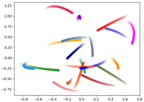
To evaluate the proposed CoGNNs, we conduct extensive experiments on three important multi-agent forecasting tasks in an online setting; that is, online simulated trajectory prediction, online human motion prediction and online traffic speed prediction, where the corresponding scenarios and data examples are sketched in Fig. 4.
In CoGNNs, we respectively use three forms of collaborative predictors in CoPUs; see section IV-B. We note the three forms of models as ‘CoGNN-AR’, ‘CoGNN-LSTM’ and ‘CoGNN-TC’, respectively. In CoGNN-AR, to compute the state, , of any collaborative pair , the order of measurement difference ; for CoGNN-LSTM and CoGNN-AR, the hidden dimension of is . The entire CoGNNs are built with CoPUs, which enable precise and stable forecasting. We train the models on one GTX-1080Ti GPU with PyTorch 1.4 framework. The learning rates are from to for different forms of CoGNNs. We also apply gradient clipping to constrain the absolute values of gradients within for robustness.
VI-A Online simulated trajectory prediction
We first evaluate the proposed CoGNNs in online simulated particle systems, which contains several moving particles whose positions and velocities are determined by their interactions.
Dataset. In our simulated particle systems, there are particle agents, whose initial states (positions and velocities) are set randomly, moving in a 2D space with dynamic mutual interaction. The interactions among the agents could be represent as a graph structure with symmetric adjacency matrix. Here we use a simple interaction rule called ’spring’ to construct the complex systems; that is, each agent has attractions with several other agents that are randomly selected. One example of our simulated system is illustrated in Fig. 4 (a). This system was similarly used by [5], where only agents are set in a simple system. However, different from the previous work [5] which generates a set of independent trajectory sequences with fixed and known interactions, in our simulated systems, agents have randomly changed interactions with different agents to reflect dynamic and changing states online. In each interactive simulation, we change the interaction structures for times randomly; that is, the interaction adjacency matrix is randomly adjusted for times. Moreover, we conduct times of different simulation to demonstrate the effectiveness and robustness. In our experiments, along the streaming data, our CoGNNs are fed with each 10-frame clip one-by-one along time and generate the next 10-frame clip for prediction.
Baselines and evaluation metrics. We compare our CoGNNs with several methods on trajectory prediction, including NRI [5], DNRI [6] and EvolveGraph [7]. These methods are designed for the offline scenarios; thus we modify these works to be run online with the same inputs and outputs as our CoGNNs. We also adjust their hyper-parameters to be reasonable. Besides being compared to the state-of-the-art works, CoGNNs are also compared to two degenerated variants: 1) CoGNNs forecasting without collaborative graphs, i.e., ‘CoGNNs (no )’; and 2) CoGNNs training collaborative graphs via online gradient descent end-to-end in black-boxes, i.e., ‘CoGNNs (e2e )’. To evaluate various methods, we employ the average mean square errors (MSE) between the predicted locations and ground-truth of all the agents over the training/testing process.
| Prediction steps | ||||||
| Methods | 1 | 2 | 5 | 8 | 10 | |
| Baselines | ZeroV | 13.43 1.94 | 13.43 1.95 | 13.48 2.08 | 13.58 2.35 | 13.69 2.64 |
| NRI [5] | 0.56 0.16 | 0.58 0.15 | 0.60 0.18 | 1.03 0.30 | 1.59 0.46 | |
| DNRI [6] | 0.26 0.10 | 0.28 0.12 | 0.31 0.12 | 0.51 0.15 | 0.77 0.19 | |
| EvolveGraph [7] | 0.22 0.10 | 0.24 0.09 | 0.28 0.10 | 0.44 0.13 | 0.68 0.15 | |
| no | CoGNN-AR (no ) | 0.23 0.06 | 0.24 0.07 | 0.41 0.12 | 0.75 0.23 | 1.09 0.32 |
| CoGNN-LSTM (no ) | 0.16 0.04 | 0.16 0.05 | 0.20 0.05 | 0.40 0.14 | 0.61 0.16 | |
| CoGNN-TC (no ) | 0.19 0.08 | 0.23 0.11 | 0.24 0.11 | 0.42 0.16 | 0.63 0.18 | |
| e2e | CoGNN-AR (e2e ) | 0.20 0.04 | 0.21 0.06 | 0.37 0.15 | 0.74 0.22 | 1.06 0.34 |
| CoGNN-LSTM (e2e ) | 0.17 0.06 | 0.16 0.06 | 0.19 0.07 | 0.37 0.13 | 0.60 0.18 | |
| CoGNN-TC (e2e ) | 0.15 0.05 | 0.18 0.07 | 0.20 0.07 | 0.36 0.12 | 0.58 0.17 | |
| Ours | CoGNN-AR | 0.19 0.06 | 0.20 0.06 | 0.37 0.12 | 0.70 0.21 | 1.01 0.30 |
| CoGNN-LSTM | 0.15 0.05 | 0.15 0.06 | 0.19 0.05 | 0.35 0.10 | 0.59 0.17 | |
| CoGNN-TC | 0.16 0.06 | 0.18 0.05 | 0.18 0.06 | 0.35 0.12 | 0.56 0.16 | |
Results. For various methods, Table I presents the average forecasting results over the online learning processes, where we show the prediction performance at prediction steps of the generated 10-frame clips, respectively. Since all the models are run on different interaction systems, the mean values and standard deviations of the prediction MSEs are presented for comparison. We see that, 1) compared to the state-of-the-art methods, our CoGNNs achieve more precise forecasting and outperform the baselines, especially CoGNN-LSTM and CoGNN-TC achieve much more effective prediction at various prediction steps; 2) compared to the model variants, ‘no ’ and ‘e2e ’, the proposed CoGNNs consistently outperforms these two variants, demonstrating the importance and effectiveness of our intepretable collaborative graphs and the exponentiated update strategy.
VI-B Online human motion prediction
We next conduct experiments on online human motion prediction to verify the effectiveness of our CoGNN.
Dataset. Various models are trained and tested on two motion capture datasets: Human3.6M (H3.6M) [61] and CMU Mocap11 1 http://mocap.cs.cmu.edu/. H3.6M contains classes of activities. There are body joints with their 3D coordinates. An examplar motion clip in H3.6M is shown in Fig. 4 (b). CMU Mocap contains activities with joints. Following the previous settings [26, 62, 15], we downsample all motion sequences along time by two for both datasets. We take the motion clips of the past ms ( frames) as input, and forecast the future ms.
| Motions | Walking | Eating | Smoking | Discussion | |||||||||||||
|---|---|---|---|---|---|---|---|---|---|---|---|---|---|---|---|---|---|
| Methods | 80 | 160 | 320 | 400 | 80 | 160 | 320 | 400 | 80 | 160 | 320 | 400 | 80 | 160 | 320 | 400 | |
| Baselines | Res-sup [26] | 23.0 | 32.1 | 37.8 | 44.4 | 20.6 | 30.2 | 37.1 | 46.0 | 23.2 | 27.6 | 35.8 | 42.7 | 30.1 | 41.8 | 46.8 | 52.0 |
| NRI [5] | 21.6 | 30.4 | 36.0 | 42.4 | 19.5 | 28.7 | 36.4 | 42.5 | 22.4 | 26.8 | 33.2 | 40.1 | 28.7 | 39.3 | 44.9 | 51.3 | |
| CSM [62] | 22.1 | 31.5 | 39.4 | 43.3 | 19.9 | 29.1 | 39.7 | 43.9 | 21.3 | 26.5 | 32.4 | 38.6 | 31.2 | 38.0 | 44.4 | 50.8 | |
| Traj-GCN [15] | 22.9 | 30.1 | 38.9 | 43.6 | 19.0 | 24.9 | 35.8 | 38.6 | 19.7 | 25.3 | 28.2 | 35.9 | 24.1 | 36.2 | 43.4 | 47.3 | |
| DNRI [6] | 22.3 | 31.8 | 39.2 | 43.7 | 19.3 | 27.6 | 36.7 | 40.5 | 20.5 | 26.3 | 29.1 | 36.7 | 26.8 | 37.2 | 43.8 | 49.0 | |
| DMGNN [17] | 22.6 | 31.1 | 39.2 | 44.1 | 18.2 | 24.2 | 32.5 | 39.2 | 19.9 | 24.3 | 27.8 | 35.7 | 24.6 | 35.8 | 43.4 | 49.5 | |
| HisRep [63] | 22.6 | 29.0 | 37.3 | 42.1 | 17.3 | 22.5 | 33.6 | 37.3 | 19.2 | 25.4 | 29.9 | 36.3 | 22.8 | 33.6 | 40.7 | 46.5 | |
| EvolveGraph [7] | 22.2 | 30.7 | 38.3 | 43.5 | 18.1 | 23.8 | 34.3 | 38.9 | 20.4 | 26.0 | 29.7 | 37.1 | 24.2 | 34.7 | 42.9 | 48.4 | |
| no | CoGNN-AR (no ) | 26.2 | 39.9 | 62.3 | 65.4 | 20.3 | 27.8 | 43.0 | 48.7 | 23.2 | 30.5 | 46.0 | 52.7 | 24.8 | 35.6 | 55.7 | 63.7 |
| CoGNN-LSTM (no ) | 23.3 | 23.9 | 29.8 | 40.1 | 19.8 | 20.0 | 26.4 | 35.0 | 20.3 | 20.8 | 28.0 | 33.9 | 29.5 | 30.0 | 40.6 | 48.9 | |
| CoGNN-TC (no ) | 25.8 | 27.3 | 37.2 | 47.2 | 19.6 | 20.1 | 30.1 | 38.3 | 17.8 | 19.1 | 29.7 | 36.3 | 22.2 | 25.3 | 36.7 | 48.3 | |
| e2e | CoGNN-AR (e2e ) | 24.9 | 35.1 | 50.5 | 57.9 | 17.6 | 26.8 | 38.7 | 40.3 | 22.3 | 28.2 | 43.6 | 48.7 | 24.9 | 34.3 | 51.7 | 58.6 |
| CoGNN-LSTM (e2e ) | 23.5 | 23.7 | 33.7 | 40.9 | 18.4 | 17.0 | 27.6 | 34.1 | 19.4 | 20.0 | 27.3 | 24.2 | 28.4 | 29.6 | 40.1 | 47.5 | |
| CoGNN-TC (e2e ) | 22.6 | 25.2 | 35.3 | 41.7 | 18.3 | 19.9 | 29.2 | 35.7 | 18.0 | 18.8 | 28.4 | 35.5 | 22.0 | 26.7 | 36.1 | 47.5 | |
| Ours | CoGNN-AR | 22.3 | 33.7 | 51.5 | 56.8 | 16.6 | 23.0 | 36.5 | 41.5 | 19.5 | 27.7 | 41.6 | 45.4 | 24.1 | 30.1 | 50.4 | 58.0 |
| CoGNN-LSTM | 22.6 | 23.3 | 33.6 | 40.7 | 18.2 | 19.2 | 26.1 | 33.7 | 19.7 | 19.4 | 25.2 | 33.8 | 28.7 | 29.3 | 38.9 | 47.3 | |
| CoGNN-TC | 21.5 | 21.4 | 31.0 | 39.7 | 16.8 | 16.2 | 28.7 | 36.0 | 16.4 | 16.6 | 26.6 | 33.6 | 19.9 | 18.5 | 34.1 | 45.2 | |
| Motions | Average | ||||
|---|---|---|---|---|---|
| Methods | 80 | 160 | 320 | 400 | |
| Baselines | Res-sup [26] | 22.9 | 30.7 | 40.4 | 47.4 |
| CSM [62] | 21.0 | 28.5 | 35.6 | 41.7 | |
| NRI [5] | 19.7 | 26.7 | 33.6 | 41.1 | |
| Traj-GCN [15] | 17.3 | 24.5 | 31.8 | 37.9 | |
| DNRI [6] | 18.3 | 25.5 | 32.4 | 38.9 | |
| DMGNN [17] | 16.8 | 23.8 | 30.6 | 37.7 | |
| HisRep [63] | 15.6 | 21.9 | 28.7 | 35.2 | |
| EvolveGraph [7] | 17.0 | 24.1 | 33.4 | 38.6 | |
| no | CoGNN-AR (no ) | 27.1 | 34.7 | 52.7 | 57.0 |
| CoGNN-LSTM (no ) | 18.6 | 21.0 | 30.0 | 37.2 | |
| CoGNN-TC (no ) | 17.0 | 19.1 | 28.4 | 34.7 | |
| e2e | CoGNN-AR (e2e ) | 23.1 | 30.6 | 45.4 | 51.2 |
| CoGNN-LSTM (e2e ) | 16.9 | 18.7 | 24.6 | 30.2 | |
| CoGNN-TC (e2e ) | 16.4 | 18.2 | 25.4 | 31.4 | |
| Ours | CoGNN-AR | 21.6 | 28.5 | 43.5 | 50.3 |
| CoGNN-LSTM | 16.7 | 17.7 | 23.3 | 29.0 | |
| CoGNN-TC | 15.4 | 17.2 | 23.8 | 28.5 | |
Baselines and evaluation metrics. We compare our model to state-of-the-art works, including two non-graph methods, Res-sup [26] and CSM [62], and six graph-based methods, NRI [5], Traj-GCN [15], DNRI [6], DMGNN [17], HisRep [63] and EvolveGraph [7]. For these offline methods, we also adjust them to take the same streaming data as our CoGNNs and generate future poses as effectively as possible in an online setting. For evaluation, we calculate the Mean Per Joint Postion Error (MPJPE) between each predicted pose and the corresponding ground-truth.
Results. We first evaluate various methods on H3.6M. Besides being compared to the state-of-the-art works, CoGNNs are also compared to two degenerated variants: i.e., ‘CoGNN (no )’ and ‘CoGNN (e2e )’; see introduction in the experiments of online simulated trajectory prediction. Table II shows the forecasting MPJPEs on 4 representative actions: ‘Walking’, ‘Eating’, ‘Smoking’ and ‘Discussion’, presenting the average MPJPEs at the future ms, ms, ms and ms. We see that, 1) compared to the state-of-the-art methods, our CoGNNs achieve more precise forecasting and outperform the baselines; 2) compared to the model variants, ‘no ’ and ‘e2e ’, the proposed CoGNNs consistently outperforms these two variants, demonstrating the importance and effectiveness of our intepretable collaborative graphs and the exponentiated update strategy. See the forecasting results of another 11 actions in Appendix.
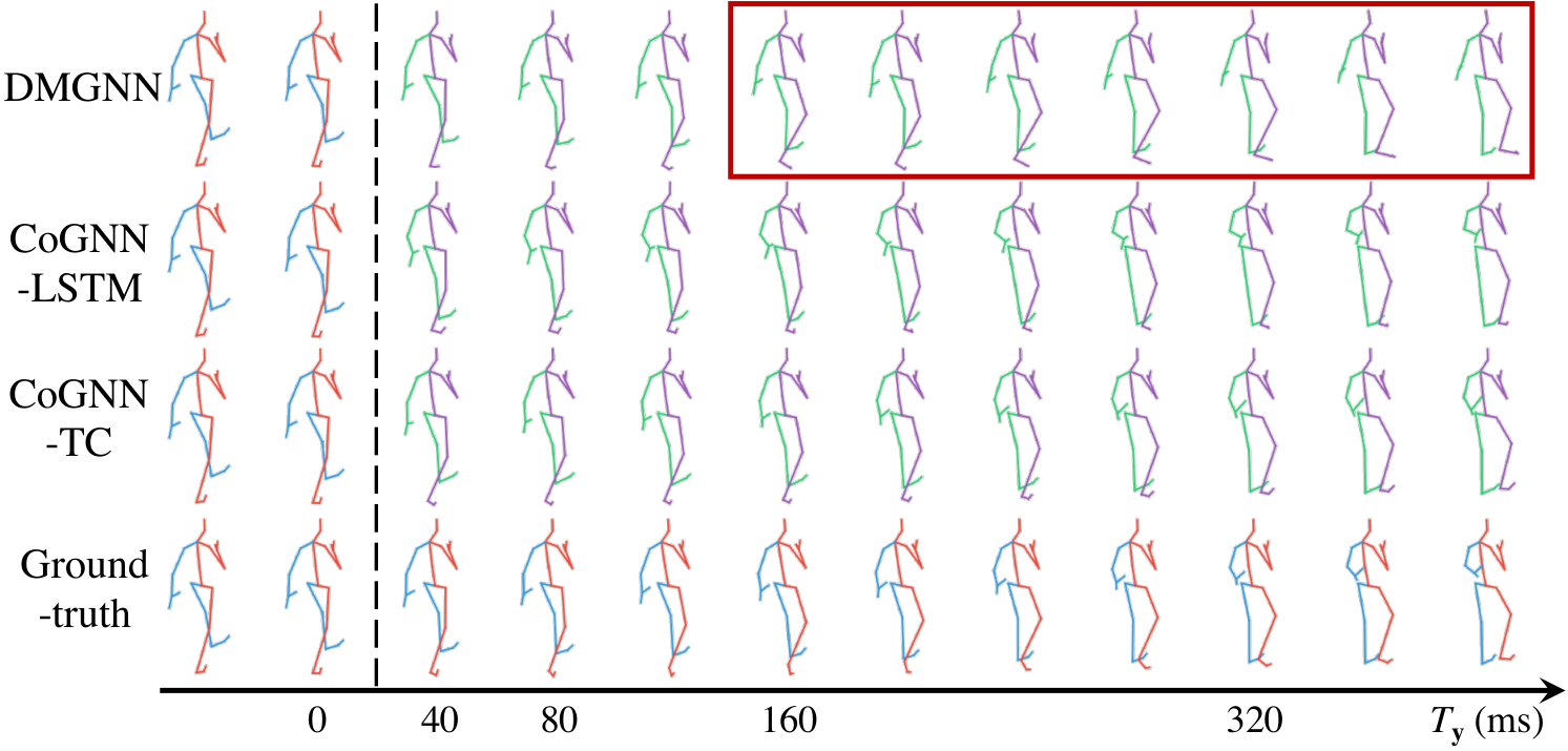
To further qualitatively evaluate our CoGNNs, we visualize the future poses produced by various methods for human motion prediction on H3.6M dataset. We illustrate the motions of a clip of ‘Walking’ within the future 400 ms, which are predicted by DMGNN [17], CoGNN-LSTM and CoGNN-TC; see Fig. 5. We see that, for the baseline model, DMGNN, there are large errors after the 160th ms of the prediction time, where the left arm on the human body cannot bend flexibly. As for the CoGNN-LSTM and CoGNN-TC, the generated poses are much closet to the ground-truths than the DMGNN model. Moreover, we note that, the illustrated human poses is the predicted samples at one certain iteration step. To evaluate the online prediction system, we should focus more on the continuous performance and the prediction errors during the whole online learning process.
Additionally, We also various methods on another large-scale datatset, CMU Mocap, for online motion prediction. The average prediction results (MPJPE) across all the actions at the future ms ms ms and ms are presented in Table III. We see that, 1) the proposed CoGNN models outperform the state-of-the-art methods with a large margin; 2) the proposed versions of CoGNNs achieve consistent better performances than the other two types of model variants to show the effectiveness of our collaborative mechanism. The detailed forecasting results of each class of activities are presented in Appendix.
| Datasets | METR-LA | PeMS-BAY | PeMS-D4 | PeMS-D8 | |||||||||
|---|---|---|---|---|---|---|---|---|---|---|---|---|---|
| Methods | MAE | RMSE | MAPE | MAE | RMSE | MAPE | MAE | RMSE | MAPE | MAE | RMSE | MAP | |
| Baselines | ST-GCN [14] | 5.68 | 8.92 | 13.0% | 3.09 | 6.57 | 7.7% | 37.28 | 46.44 | 30.5% | 30.49 | 39.57 | 24.8% |
| DCRNN [18] | 5.45 | 8.76 | 12.6% | 3.07 | 6.69 | 7.8% | 37.67 | 46.95 | 31.1% | 31.31 | 39.35 | 25.4% | |
| ASTGCN [13] | 4.66 | 7.43 | 11.7% | 2.51 | 4.29 | 6.0% | 32.15 | 43.72 | 28.8% | 28.85 | 36.97 | 23.0% | |
| G-WaveNet [31] | 4.42 | 7.10 | 11.2% | 2.31 | 4.07 | 5.3% | 28.58 | 39.59 | 25.6% | 27.81 | 36.03 | 19.8% | |
| STSGCN [4] | 4.73 | 7.62 | 11.6% | 2.44 | 4.31 | 6.8% | 23.82 | 30.85 | 18.9% | 24.47 | 33.11 | 16.4% | |
| AGCRN [64] | 4.19 | 6.40 | 8.3% | 2.16 | 3.74 | 4.7% | 19.65 | 28.54 | 16.0% | 22.72 | 29.03 | 13.4% | |
| no | CoGNN-AR (no ) | 4.42 | 6.61 | 8.8% | 1.72 | 2.65 | 4.1% | 19.37 | 28.02 | 17.3% | 16.92 | 26.61 | 12.7% |
| CoGNN-LSTM (no ) | 6.08 | 8.35 | 14.6% | 2.74 | 3.68 | 4.4% | 27.45 | 35.14 | 19.3% | 20.12 | 29.73 | 13.7% | |
| CoGNN-TC (no ) | 3.61 | 5.89 | 8.0% | 1.43 | 2.41 | 3.0% | 20.27 | 29.48 | 16.1% | 16.99 | 24.14 | 11.9% | |
| Ours | CoGNN-AR | 4.09 | 6.22 | 8.3% | 1.59 | 2.42 | 3.8% | 19.07 | 26.94 | 15.3% | 15.75 | 23.74 | 11.4% |
| CoGNN-LSTM | 5.04 | 7.28 | 13.4% | 2.21 | 3.52 | 4.2% | 26.95 | 32.31 | 18.9% | 19.62 | 28.87 | 13.1% | |
| CoGNN-TC | 3.46 | 5.75 | 7.8% | 1.36 | 2.24 | 2.8% | 18.93 | 27.71 | 14.7% | 15.51 | 22.35 | 10.8% | |
VI-C Online traffic speed prediction
Furthermore, the proposed CoGNNs are also evaluated on the tasks of online traffic speed prediction.
Datasets. We conduct experiments on four large-scale traffic datasets in the real world, including the traffic data of Los Angeles county [65] or different regions of the California highway [66]:
METR-LA contains traffic speed collected by 207 sensors around Los Angeles from March to June in 2012.
PeMS-BAY contains traffic speed at Bay Area collected by 325 sensors on CalTrans Performance Measurement System (PeMS) from Jan. to May in 2017.
PeMS-D4 contains traffic speed collected by 307 sensors at San Francisco from Jan. to Feb. in 2018.
PeMS-D8 contains traffic speed collected by 170 sensors in San Bernardino from July to Aug. in 2016.
We illustrate the traffic speed distribution of METR-LA in Fig. 4 (c) as an example, where we denote that each sensor captures the dynamic traffic speed along time. For these datasets, we aggregate the data sequence into 5-minute intervals from 30-second frequency. We take the past -frame-length ( hour) sequence as the input and forecast the next frames.
Baselines and evaluation metrics. To evaluate the effectiveness our CoGNNs on the online traffic speed prediction, we introduce several state-of-the-art models for comparison,including ST-GCN [14], DCRNN [18], ASTGCN [13], G-WaveNet [31], STSGCN [4] and AGCRN [64]. To test various methods, we utilize three metrics, which are mean absolute error (MAE), root mean square error (RMSE) and mean absolute percentage error (MAPE) over the whole iterative training and test process.
Results. We compare CoGNNs to various algorithms on four datasets. We also test the degenerated variants of CoGNNs without collaborative graphs, i.e., CoGNNs (no ). We evaluate on the mean MAE, mean RMSE and mean MAPE as shown in Table IV. We see that, 1) compared to the previous works, our CoGNNs obtain the lowest errors on all the datasets; 2) compared to the model variants without collaborative graphs, the complete CoGNNs also achieve the much better prediction performances. The detailed traffic forecasting at different prediction time are presented in Appendix.
VI-D Model analysis
Regrets of various forms of CoGNNs.
| (a) Regret curves. | (b) Effects of learning rates. |
According to our theoretical regret analysis, the static regrets converge with . Here we compute and visualize the static regrets of different forms of CoGNNs to verify our analysis. For online motion prediction on H3.6M, we illustrate the regret curves along time within iterations; see Fig. 6 (a). The regrets of three forms of CoGNNs could converge to very low values within approximately iterations. Additionally, the regret curves reflect that CoGNNs quickly close the performance gaps with the models that only consider the best collaborative pairs, showing the effectiveness and interpretation of our CoPUs.
Effect of learning rate . The learning rate affects the training of the collaborative predictor and the collaborative graph in each CoPU. Here we vary the learning rate from to to test the model performance for online motion prediction on H3.6M. The mean MPJPEs of different forms of CoGNNs are illustrated in Fig. 6 (b). We see that, CoGNN-AR, CoGNN-LSTM and CoGNN-TC achieve their best performance when is , and , respectively. CoGNN-AR tends to be more stable with various than others; CoGNN-LSTM and CoGNN-TC obtain better performance given the reasonable .
Effect of number of CoPUs in CoGNNs.
| Methods | 1 CoPU | 2 CoPUs | 3 CoPUs | 4 CoPUs |
|---|---|---|---|---|
| CoGNN-AR | 38.16 | 34.42 | 34.46 | 35.15 |
| CoGNN-LSTM | 28.48 | 26.73 | 27.47 | 26.92 |
| CoGNN-TC | 26.07 | 24.39 | 24.74 | 25.03 |
Here we analyze how different numbers of CoPUs in the CoGNN architectures affect the performance. We test different forms of CoGNNs with to CoPUs for online human motion prediction on H3.6M. The mean MPJPEs are presented in Table V. For three forms of CoGNNs, two CoPUs help to achieve the lowest MPJPEs, which outperform the models with only one CoPU to different extents, showing the effectiveness of the progressively refinement. For or CoPUs, the model performance shows sub-par results due to the slight over-smoothing, but it still converges to stable values.
Visualization of the learned collaborative graphs. To show that our model effectively captures the implicit systematic dependencies by learning collaborative graphs, here we visualize the learned collaborative graphs on the various tasks of online simulated trajectory prediction, human motion prediction and traffic speed prediction, respectively.
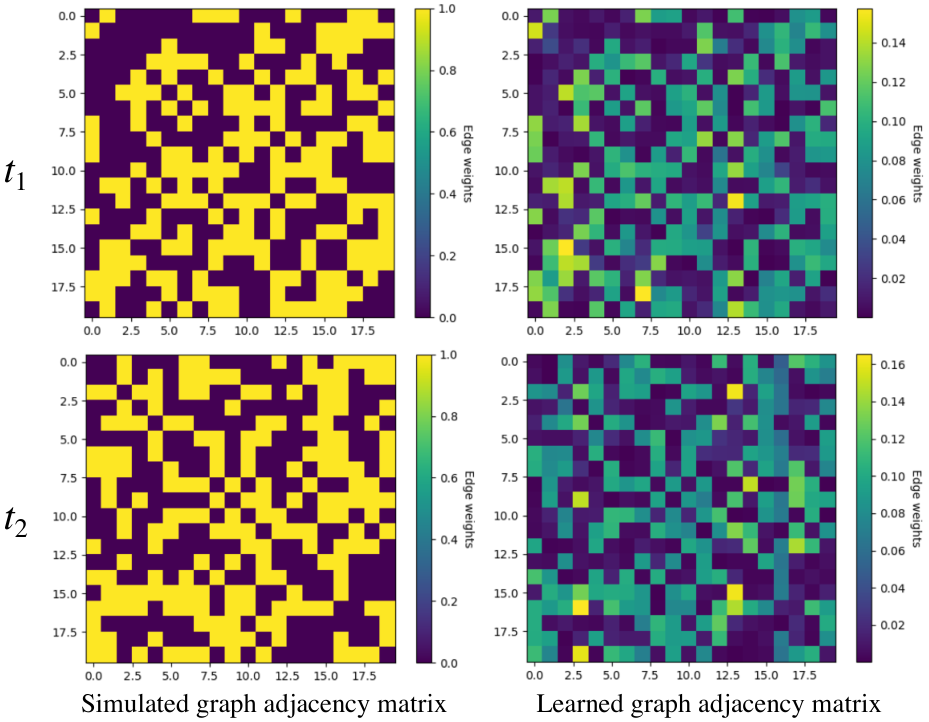
We first visualize the collaborative graphs for online simulated trajectory prediction. We compare the learned collaborative graphs and the predefined interactions that are used to simulate the particle interaction systems. We illustrate the adjacency matrices of both simulated graphs and learned graphs. To reflect that our model could adapt to the changing states of the interaction systems, we show the learned graphs at different iteration steps during the online learning process. The adjacency matrices are illustrated in Fig. 7. We see that, at one iteration step, or , the learned collaborative graph captures similar topologies to the simulated graphs with weighted edges to different extents. At different iteration steps, the collaborative graphs could adapt to the changing simulated interaction structures. Note that the element values of the graph adjacency matrices are not similar due to the normalization in our weight update algorithm, while we focus more on the visual similarity of topologies. In this way, we verify that the collaborative graph could reasonably depict the implicit interactions in the complex systems.
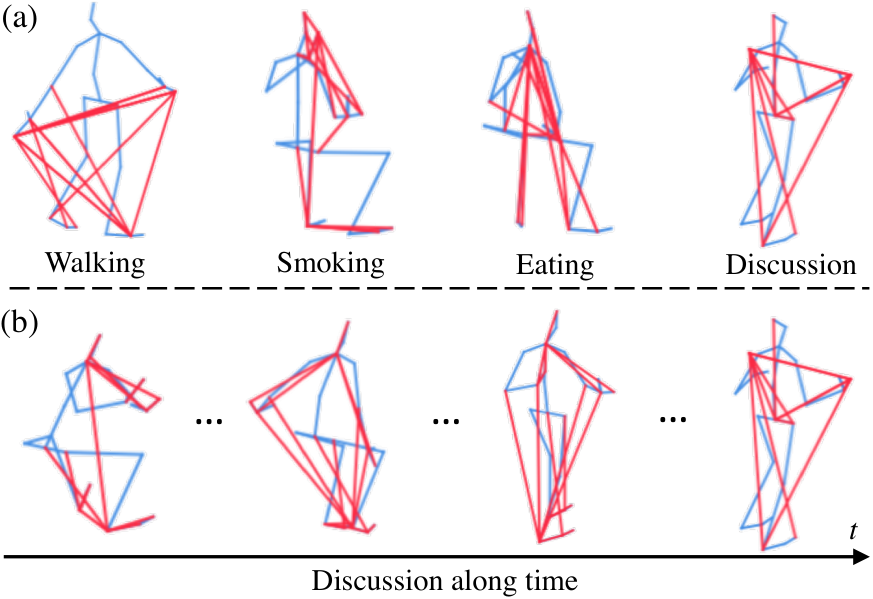
Here we visualize the learned collaborative graphs on H3.6M dataset. We use red segments to plot the graph edges whose weights are larger than on human poses. Since any edge weights range from to , and most of them are lower than , thus the plotted edges show the important collaborative pairs, i.e., the important influence between two agents. The graphs are illustrated in Fig. 8. In plot (a), different actions have different graphs, indicating distinct relations on specific actions; for example, arms and legs affect across left and right for walking, while hands are highly related to other joints for eating and smoking. In plot (b), we show the dynamic graphs changing along time during discussion.
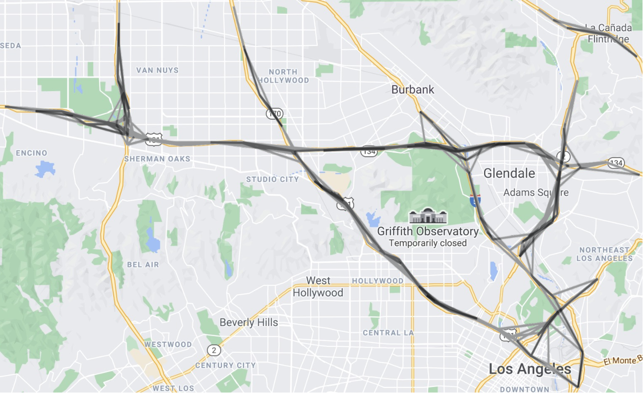
We also show the learned collaborative graph for online traffic speed prediction. As an example, we show the learned graph on METR-LA dataset. We illustrate the edges whose collaborative weights are larger than in Fig. 9, which reflects the most important collaborative effects among the nodes to some extent. We see that, the traffic speed data collected by different sensors are mainly affected by their geographically nearby traffic. For example, a certain node on a single long high-way is mainly affected by other nodes on the same high-way, because a single long high-way could be regarded as an isolated systems, in which the the vehicles move and stop collaboratively. Moreover, near the intersections or the traffic circles, one node tends to be affected by the traffic around across roads, since many vehicles perform agglomeration effects in these local regions. Fig. 9 shows a reasonable structure to depict the collaborative effects. The collaborative graphs for online human motion prediction have been illustrated in Figure 3 of our main text. Different from the human motion data, in a traffic scenario, the interactions and relations between two nodes with a relatively long distance is usually weak. That is because traffic data has very strong spatial location attributes, and higher synergy tends to appear in more local areas, such as local congestion during peak hours; and two nodes farther apart are difficult to affect each other because of the decay of collaborative effects along distances.
VII Conclusion
We develop a novel method to predict the future statuses of a multi-agent system online. We propose a novel CoPU, which uses a collaborative graph to aggregate multiple collaborative predictors that learn dynamics from collaborative pairs. The collaborative graph depicts the influence level of collaborative pairs, which are adjusted with the guidance from an explicit objective. The regret analysis show that our method achieves the similar performance with the best single collaborative predictor. Multiple CoPUs are stacked as a CoGNN. Experiments demonstrate the effectiveness of our method for various multi-agent forecasting tasks.
References
- [1] A. Jahangiri and H. A. Rakha, “Applying machine learning techniques to transportation mode recognition using mobile phone sensor data,” IEEE Transactions on Intelligent Transportation Systems (TITS), vol. 16, no. 5, pp. 2406–2417, 2015.
- [2] J. Wojtusiak, T. Warden, and O. Herzog, “Machine learning in agent-based stochastic simulation: Inferential theory and evaluation in transportation logistics,” Computers & Mathematics with Applications, vol. 64, no. 12, pp. 3658 – 3665, 2012.
- [3] W. Yu, D. An, D. Griffith, Q. Yang, and G. Xu, “Towards statistical modeling and machine learning based energy usage forecasting in smart grid,” ACM SIGAPP Applied Computing Review, vol. 15, pp. 6–16, 2015.
- [4] C. Song, Y. Lin, S. Guo, and H. Wan, “Spatial-temporal synchronous graph convolutional networks: A new framework for spatial-temporal network data forecasting,” in Proceedings of the AAAI Conference on Artificial Intelligence (AAAI), 2020, pp. 914–921.
- [5] T. Kipf, E. Fetaya, K.-C. Wang, M. Welling, and R. Zemel, “Neural relational inference for interacting systems,” in Proceedings of International Conference on Machine Learning (ICML), 2018, pp. 2688–2697.
- [6] C. Graber and A. G. Schwing, “Dynamic neural relational inference,” in IEEE/CVF Conference on Computer Vision and Pattern Recognition (CVPR), 2020, pp. 8513–8522.
- [7] J. Li, F. Yang, M. Tomizuka, and C. Choi, “Evolvegraph: Multi-agent trajectory prediction with dynamic relational reasoning,” in Advances in Neural Information Processing Systems (NeurIPS), 2020, pp. 19 783–19 794.
- [8] S. C. H. Hoi, D. Sahoo, J. Lu, and P. Zhao, “Online learning: A comprehensive survey,” CoRR, vol. abs/1802.02871, 2018.
- [9] E. Zivor and J. Wang, “Vector autoregressive models for multivariate time series,” Modeling Financial Time Series with S-PLUS®, pp. 385–429, 2006.
- [10] A. Lehrmann, P. Gehler, and S. Nowozin, “Efficient nonlinear markov models for human motion,” in The IEEE Conference on Computer Vision and Pattern Recognition (CVPR), 2014, pp. 1314–1321.
- [11] K. P. Vishwakarma, “Prediction of economic time-series by means of the kalman filter,” International Journal of Systems Science, 1970.
- [12] S. Hochreiter and J. Schmidhuber, “Long short-term memory,” Neural computation, vol. 9, no. 8, pp. 1735–1780, 1997.
- [13] S. Guo, Y. Lin, N. Feng, C. Song, and H. Wan, “Attention based spatial-temporal graph convolutional networks for traffic flow forecasting,” in AAAI Conference on Artificial Intelligence (AAAI), 2019, pp. 922–929.
- [14] B. Yu, H. Yin, and Z. Zhu, “Spatio-temporal graph convolutional networks: A deep learning framework for traffic forecasting,” in Proceedings of International Joint Conference on Artificial Intelligence (IJCAI), 2018, pp. 3634–3640.
- [15] W. Mao, M. Liu, M. Salzmann, and H. Li, “Learning trajectory dependencies for human motion prediction,” in Proceedings of the IEEE/CVF International Conference on Computer Vision (ICCV), 2019, pp. 9489–9497.
- [16] Q. Cui, H. Sun, and F. Yang, “Learning dynamic relationships for 3d human motion prediction,” in Proceedings of the IEEE/CVF Conference on Computer Vision and Pattern Recognition (CVPR), 2020, pp. 6519–6527.
- [17] M. Li, S. Chen, Y. Zhao, Y. Zhang, Y. Wang, and Q. Tian, “Dynamic multiscale graph neural networks for 3d skeleton based human motion prediction,” in Proceedings of the IEEE/CVF Conference on Computer Vision and Pattern Recognition (CVPR), 2020, pp. 214–223.
- [18] Y. Li, R. Yu, C. Shahabi, and Y. Liu, “Diffusion convolutional recurrent neural network: Data-driven traffic forecasting,” in International Conference on Learning Representations (ICLR), 2018.
- [19] M. Li, S. Chen, X. Chen, Y. Zhang, Y. Wang, and Q. Tian, “Actional-structural graph convolutional networks for skeleton-based action recognition,” in Proceedings of the IEEE/CVF Conference on Computer Vision and Pattern Recognition (CVPR), 2019, pp. 3595–3603.
- [20] Y. Hu, S. Chen, Y. Zhang, and X. Gu, “Collaborative motion prediction via neural motion message passing,” in Proceedings of the IEEE/CVF Conference on Computer Vision and Pattern Recognition (CVPR), 2020, pp. 6319–6328.
- [21] L. Shi, Y. Zhang, J. Cheng, and H. Lu, “Two-stream adaptive graph convolutional networks for skeleton-based action recognition,” in Proceedings of the IEEE/CVF Conference on Computer Vision and Pattern Recognition (CVPR), 2019, pp. 12 026–12 035.
- [22] B. Williams and L. Hoel, “Modeling and forecasting vehicular traffic flow as a seasonal arima process: Theoretical basis and empirical results,” Journal of Transportation Engineering, vol. 129, no. 6, pp. 664–672, 2003.
- [23] J. Wang, A. Hertzmann, and D. Fleet, “Gaussian process dynamical models,” in Advances in Neural Information Processing Systems (NeurIPS), 2006, pp. 1441–1448.
- [24] G. Taylor and G. Hinton, “Factored conditional restricted Boltzmann machines for modeling motion style,” in International Conference on Machine Learning (ICML), 2009, pp. 1025–1032.
- [25] S. S. Rangapuram, M. W. Seeger, J. Gasthaus, L. Stella, Y. Wang, and T. Januschowski, “Deep state space models for time series forecasting,” in Advances in Neural Information Processing Systems (NeurIPS), 2018, pp. 7785–7794.
- [26] J. Martinez, M. Black, and J. Romero, “On human motion prediction using recurrent neural networks,” in The IEEE Conference on Computer Vision and Pattern Recognition (CVPR), 2017, pp. 4674–4683.
- [27] L.-Y. Gui, Y.-X. Wang, X. Liang, and J. M. F. Moura, “Adversarial geometry-aware human motion prediction,” in The European Conference on Computer Vision (ECCV), 2018, pp. 786–803.
- [28] G. Lai, W.-C. Chang, Y. Yang, and H. Liu, “Modeling long- and short-term temporal patterns with deep neural networks,” in International ACM SIGIR Conference on Research & Development in Information Retrieval (SIGIR), 2018, pp. 95–104.
- [29] S. Bai, J. Z. Kolter, and V. Koltun, “An empirical evaluation of generic convolutional and recurrent networks for sequence modeling,” CoRR, vol. abs/1803.01271, 2018.
- [30] A. Jain, A. Zamir, S. Savarese, and A. Saxena, “Structural-rnn: Deep learning on spatio-temporal graphs,” in The IEEE Conference on Computer Vision and Pattern Recognition (CVPR), 2016, pp. 5308–5317.
- [31] Z. Wu, S. Pan, G. Long, J. Jiang, and C. Zhang, “Graph wavenet for deep spatial-temporal graph modeling,” in Proceedings of International Joint Conference on Artificial Intelligence (IJCAI), 2019, pp. 1907–1913.
- [32] M. Li, S. Chen, Y. Zhang, and I. Tsang, “Graph cross networks with vertex infomax pooling,” in Advances in Neural Information Processing Systems (NeurIPS), 2020.
- [33] P. D. Dobson and A. J. Doig, “Distinguishing enzyme structures from non-enzymes without alignments,” Journal of Molecular Biology (JMB), vol. 330, no. 4, pp. 771–783, 2003.
- [34] T. Kipf and M. Welling, “Semi-supervised classification with graph convolutional networks,” in International Conference on Learning Representations (ICLR), 2017.
- [35] P. Veličković, G. Cucurull, A. Casanova, A. Romero, P. Liò, and Y. Bengio, “Graph attention networks,” in International Conference on Learning Representations (ICLR), 2018.
- [36] S. Liu, M. Sun, L. Feng, H. Qiao, S. Chen, and Y. Liu, “Social neighborhood graph and multigraph fusion ranking for multifeature image retrieval,” IEEE Transactions on Neural Networks and Learning Systems (TNNLS), vol. 32, no. 3, pp. 1389–1399, 2021.
- [37] L. C. B. Torres, C. L. Castro, F. Coelho, and A. P. Braga, “Large margin gaussian mixture classifier with a gabriel graph geometric representation of data set structure,” IEEE Transactions on Neural Networks and Learning Systems (TNNLS), vol. 32, no. 3, pp. 1400–1406, 2021.
- [38] J. Bruna, W. Zaremba, A. Szlam, and Y. LeCun, “Spectral networks and locally connected networks on graphs,” in International Conference on Learning Representations (ICLR), 2014.
- [39] M. Defferrard, X. Bresson, and P. Vandergheynst, “Convolutional neural networks on graphs with fast localized spectral filtering,” in Advances in Neural Information Processing Systems (NeurIPS), 2016, pp. 3844–3852.
- [40] W. Hamilton, Z. Ying, and J. Leskovec, “Inductive representation learning on large graphs,” in Advances in Neural Information Processing Systems (NeurIPS), 2017, pp. 1024–1034.
- [41] M. Niepert, M. Ahmed, and K. Kutzkovl, “Learning convolutional neural networks for graphs,” in Proceedings of the International Conference on Machine Learning (ICML), 2016.
- [42] Y. Li, D. Tarlow, M. Brockschmidt, and R. Zemel, “Gated graph sequence neural networks,” in International Conference on Learning Representations (ICLR), 2016.
- [43] H. Dai, B. Dai, and L. Song, “Discriminative embeddings of latent variable models for structured data,” in Proceedings of the International Conference on Machine Learning (ICML), 2016.
- [44] K. Xu, W. Hu, J. Leskovec, and S. Jegelka, “How powerful are graph neural networks?” in International Conference on Learning Representations (ICLR), 2019.
- [45] X. Xu, T. Wang, Y. Yang, A. Hanjalic, and H. T. Shen, “Radial graph convolutional network for visual question generation,” IEEE Transactions on Neural Networks and Learning Systems, vol. 32, no. 4, pp. 1654–1667, 2021.
- [46] S. Thrun, “Lifelong learning algorithms,” Learning to Learn, pp. 181–209, 1998.
- [47] J. Lu, D. Sahoo, P. Zhao, and S. C. H. Hoi, “Sparse passive-aggressive learning for bounded online kernel methods,” ACM transactions on intelligent systems, vol. 9, no. 4, pp. 216–242, 2018.
- [48] J. Kivinen, A. J. Smola, and R. C. Williamson, “Online learning with kernels,” IEEE Transactions on Signal Processing, vol. 52, no. 8, pp. 2165–2176, 2004.
- [49] O. Dekel, S. Shalev-Shwartz, and Y. Singer, “The forgetron: A kernel-based perceptron on a budget,” SIAM Journal on Computing, vol. 37, no. 5, p. 1342–1372, 2008.
- [50] Z. Wang, K. Crammer, and S. Vucetic, “Breaking the curse of kernelization: Budgeted stochastic gradient descent for large-scale svm training,” Journal of Machine Learning Research, vol. 13, no. 100, pp. 3103–3131, 2012.
- [51] J. Zhang, H. Ning, X. Jing, and T. Tian, “Online kernel learning with adaptive bandwidth by optimal control approach,” IEEE Transactions on Neural Networks and Learning Systems (TNNLS), vol. 32, no. 5, pp. 1920–1934, 2021.
- [52] J. Lu, S. C. Hoi, J. Wang, P. Zhao, and Z.-Y. Liu, “Large scale online kernel learning,” Journal of Machine Learning Research, vol. 17, no. 47, pp. 1–43, 2016.
- [53] P. Bouboulis, S. Chouvardas, and S. Theodoridis, “Online distributed learning over networks in rkh spaces using random fourier features,” IEEE Transactions on Signal Processing, vol. 66, no. 7, pp. 1920–1932, 2018.
- [54] Y. Ding, C. Liu, P. Zhao, and S. C. H. Hoi, “Large scale kernel methods for online auc maximization,” in IEEE International Conference on Data Mining (ICDM), 2017, pp. 91–100.
- [55] Y. Shen, T. Chen, and G. B. Giannakis, “Random feature-based online multi-kernel learning in environments with unknown dynamics,” Journal of Machine Learning Research, vol. 20, no. 22, pp. 1–36, 2019.
- [56] Y. Xiu, J. Li, H. Wang, Y. Fang, and C. Lu, “Pose flow: Efficient online pose tracking,” in British Machine Vision Conference (BMVC), 2018, pp. 1–12.
- [57] J. Bütepage, H. Kjellström, and D. Kragic, “Anticipating many futures: Online human motion prediction and generation for human-robot interaction,” in International Conference on Robotics and Automation (ICRA), 2018, pp. 4563–4570.
- [58] F. Marchetti, F. Becattini, L. Seidenari, and A. D. Bimbo, “Mantra: Memory augmented networks for multiple trajectory prediction,” in IEEE/CVF Conference on Computer Vision and Pattern Recognition (CVPR), 2020, pp. 7143–7152.
- [59] Y. Cai, L. Huang, Y. Wang, T.-J. Cham, J. Cai, J. Yuan, J. Liu, X. Yang, Y. Zhu, X. Shen, D. Liu, J. Liu, and N. M. Thalmann, “Learning progressive joint propagation for human motion prediction,” in European Conference on Computer Vision (ECCV), 2020, pp. 226–242.
- [60] E. Hazan, “Introduction to online convex optimization,” Foundations and Trends in Machine Learning, vol. 2, no. 3-4, pp. 157–325, 2016.
- [61] C. Ionescu, D. Papava, V. Olaru, and C. Sminchisescu, “Human3.6m: Large scale datasets and predictive methods for 3d human sensing in natural environments,” IEEE Transactions on Pattern Analysis and Machine Intelligence, vol. 36, no. 7, pp. 1325–1339, 2014.
- [62] C. Li, Z. Zhang, W. Sun Lee, and G. Hee Lee, “Convolutional sequence to sequence model for human dynamics,” in The IEEE Conference on Computer Vision and Pattern Recognition (CVPR), 2018, pp. 5226–5234.
- [63] W. Mao, M. Liu, and M. Salzmann, “History repeats itself: Human motion prediction via motion attention,” in European Conference on Computer Vision (ECCV), 2020, pp. 474–489.
- [64] L. Bai, L. Yao, C. Li, X. Wang, and C. Wang, “Adaptive graph convolutional recurrent network for traffic forecasting,” in Advances in Neural Information Processing Systems (NeurIPS), 2020.
- [65] H. V. Jagadish, J. Gehrke, A. Labrinidis, Y. Papakonstantinou, J. M. Patel, R. Ramakrishnan, and C. Shahabi, “Big data and its technical challenges,” Commun. ACM, vol. 57, no. 7, p. 86–94, 2014.
- [66] C. Chen, K. Petty, and A. Skabardonis, “Freeway performance measurement system: Mining loop detector data,” Transportation Research Record, vol. 1748, pp. 96–102, 2001.
![[Uncaptioned image]](2107.00894v1/msli.png) |
Maosen Li recieved the B.E. degree in optical engineering from University of Electronic Science and Technology of China (UESTC), Chengdu, China, in 2017. He is working toward the Ph.D. degree at Cooperative Meidianet Innovation Center in Shanghai Jiao Tong University since 2017. His research interests include computer vision, machine learning, graph representation learning, and video analysis. He is the reviewer of some prestigious international journals and conferences, including IEEE-TPAMI, IEEE-TNNLS, IJCV, IEEE-TMM, PR, ICML, NeurIPS and AAAI. He is a student member of the IEEE. |
![[Uncaptioned image]](2107.00894v1/sihengc.png) |
Siheng Chen is an associate professor at Shanghai Jiao Tong University. Before that, he was a research scientist at Mitsubishi Electric Research Laboratories (MERL). Before joining MERL, he was an autonomy engineer at Uber Advanced Technologies Group, working on the perception and prediction systems of self-driving cars. Before joining Uber, he was a postdoctoral research associate at Carnegie Mellon University. Chen received the doctorate in Electrical and Computer Engineering from Carnegie Mellon University in 2016, where he also received two masters degrees in Electrical and Computer Engineering and Machine Learning, respectively. He received his bachelor’s degree in Electronics Engineering in 2011 from Beijing Institute of Technology, China. Chen was the recipient of the 2018 IEEE Signal Processing Society Young Author Best Paper Award. His coauthored paper received the Best Student Paper Award at IEEE GlobalSIP 2018. He organized the special session ”Bridging graph signal processing and graph neural networks” at ICASSP 2020. His research interests include graph signal processing, graph neural networks and autonomous driving. He is a member of IEEE. |
![[Uncaptioned image]](2107.00894v1/Portraits/yanningshen.png) |
Yanning Shen received her Ph.D. degree from the University of Minnesota (UMN) in 2019. She was a finalist for the Best Student Paper Award at the 2017 IEEE International Workshop on Computational Advances in Multi-Sensor Adaptive Processing, and the 2017 Asilomar Conference on Signals, Systems, and Computers. She was selected as a Rising Star in EECS by Stanford University in 2017, and received the UMN Doctoral Dissertation Fellowship in 2018. Her research interests span the areas of machine learning, network science, data science and statistical-signal processing. |
![[Uncaptioned image]](2107.00894v1/Portraits/genjialiu.jpg) |
Genjia Liu is an undergraduate student at Shanghai Jiao Tong University since 2017. He is going to work toward the Ph.D. degree at Cooperative Medianet Innovation Center in Shanghai Jiao Tong University from 2021. His research interests include graph signal processing and graph representation learning. |
![[Uncaptioned image]](2107.00894v1/Portraits/Ivor_Card.jpg) |
Ivor Tsang is Professor of Artificial Intelligence with the University of Technology Sydney. He is also the Research Director of the Australian Artificial Intelligence Institute. His research interests include transfer learning, deep generative models, and big data analytics. In 2013, Prof Tsang received his prestigious ARC Future Fellowship for his research regarding Machine Learning on Big Data. In 2019, his JMLR paper titled ”Towards ultrahigh dimensional feature selection for big data” received the International Consortium of Chinese Mathematicians Best Paper Award. In 2020, Prof Tsang was recognized as the AI 2000 AAAI/IJCAI Most Influential Scholar in Australia for his outstanding contributions to the field of AAAI/IJCAI between 2009 and 2019. His research on transfer learning granted him the Best Student Paper Award at CVPR 2010 and the 2014 IEEE TMM Prize Paper Award. In addition, he received the IEEE TNN Outstanding 2004 Paper Award in 2007. He serves as a Senior Area Chair/Area Chair for NeurIPS, ICML, AISTATS, AAAI and IJCAI, and the Editorial Board for JMLR, MLJ, and IEEE TPAMI. |
![[Uncaptioned image]](2107.00894v1/Portraits/ZhangYa2018.jpg) |
Ya Zhang is currently a professor at the Cooperative Medianet Innovation Center, Shanghai Jiao Tong University. Her research interest is mainly in machine learning with applications to multimedia and healthcare. Dr. Zhang holds a Ph.D. degree in Information Sciences and Technology from Pennsylvania State University and a bachelor’s degree from Tsinghua University in China. Before joining Shanghai Jiao Tong University, Dr. Zhang was a research manager at Yahoo! Labs, where she led an R&D team of researchers with strong backgrounds in data mining and machine learning to improve the web search quality of Yahoo international markets. Prior to joining Yahoo, Dr. Zhang was an assistant professor at the University of Kansas with a research focus on machine learning applications in bioinformatics and information retrieval. Dr. Zhang has published more than 70 refereed papers in prestigious international conferences and journals, including TPAMI, TIP, TNNLS, ICDM, CVPR, ICCV, ECCV, and ECML. She currently holds 5 US patents and 4 Chinese patents and has 9 pending patents in the areas of multimedia analysis. She was appointed the Chief Expert for the ’Research of Key Technologies and Demonstration for Digital Media Self-organizing’ project under the 863 program by the Ministry of Science and Technology of China. She is a member of IEEE. |