Reconsidering Dependency Networks from an Information Geometry Perspective

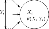
The structure of dependency networks resembles the structure of Bayesian networks. A dependency network is represented by a directed graph with $n$ nodes indexed by the numbers $0,...,n-1$. As shown in Figure 1, each node has a variable $X_{i}$ and a conditional probability table (CPT) $\theta_{i}(X_{i}|Y_{i})$, where $Y_{i}$ denotes certain variables in $X_{-i}$. We call $Y_{i}$ input variables (or simply inputs) of node $i$.

It is possible to consider that $X_{i}$ takes continuous values. In this case, $\theta_{i}$ is a density function, and CPT is implemented using a regression technique for continuous variables. However, for simplicity, we focus on the cases where $X_{i}$ takes discrete finite values in this paper.

The dependency network graph consists of edges directed from node $i$’s input variables to node $i$. Unlike the Bayesian network, the graph of a dependency network can be cyclic.

Here, we explain how to synthesize a joint distribution from CPTs owned by the nodes.

Pseudo-Gibbs sampling (Heckerman et al. 2000) is a Markov chain Monte Carlo method that is applied to synthesize a joint distribution $\pi(X)$ from CPTs owned by the nodes. The following algorithm is an example of pseudo-Gibbs sampling.

There are two ways to select a node in line 4. One is to select a node in a sequential and cyclic manner such as $0,1,...,n-1,0,1,...$. We refer to this type of pseudo-Gibbs sampling as ordered-pseudo-Gibbs sampling. The second option is to randomly select a node $i$ with probability $c_{i}$ such that

Typically, $c_{i}=1/n$ is used unless there is a particular reason (Section 2.4). We refer to this type of pseudo-Gibbs sampling as random-pseudo-Gibbs sampling. The operation in line 5 is mentioned frequently in this paper; therefore, we will refer to this operation as firing node $i$.

Let $O^{N}=\{X^{0},...,X^{N-1}\}$ be $N$ samples of output data—as a sequence of random variables—of pseudo-Gibbs sampling algorithm. Here, we assume the ergodicity of random-pseudo-Gibbs sampling. Then, the following consequences hold (Gilks et al. 1995, Chapter 3).

• •

  There uniquely exists a distribution $\pi(X)$, called stationary distribution, such that for any initial value $x^{0}$,

  $$\pi(X)=\lim_{t\to\infty}p(X^{t}|x^{0}).$$

  (4)

• •

  For any real valued function $f(X)$ that satisfies $\left<|f(X)|\right>_{\pi(X)}<\infty$,

  $$\lim_{N\to\infty}\frac{f(X^{0})+...+f(X^{N-1})}{N}=\left<f(X)\right>_{\pi(X)}\quad(a.s.).$$

  (5)

Substituting $1(X=x)$ (indicator function) for $f$ in Eq.(5), we obtain

where $N_{x}$ denotes the number of occurrences of $X^{t}=x(t=0,...,N-1)$ in the output dataset. Equation (6) implies that, even if it is not possible to know $\pi(x)$ directly, we can estimate $\pi(x)$ by a Monte Carlo method.

Ordered-pseudo-Gibbs sampling is an inhomogeneous Markov chain (Seneta 2006, Chapter 4) and does not have a stationary distribution. Even in this case, the subsequence $X^{i}X^{i+n}X^{i+2n}...$ becomes a homogeneous Markov chain and has a stationary distribution $\pi_{i}(X)$ under the assumption of ergodicity. Therefore, the limit in the left side of Eq.(6) still exists and

Contrary to pseudo-Gibbs sampling, we refer to usual Gibbs sampling as actual-Gibbs sampling in this paper. Actual-Gibbs sampling is a special case of the pseudo-Gibbs sampling such that there exists a joint distribution $p(X)$ that satisfies

for all $i$. In this case, $p$ becomes the stationary distribution because firing any node $i$ does not move $p$.

Here, we build the following rough hypothesis.

Hypothesis 1.

If every CPT is a good estimation of $p^{*}(X_{i}|X_{-i})$, then the stationary distribution of pseudo-Gibbs sampling becomes a good estimation of $p^{*}(X)$.

Hypothesis 1 plays the central role in dependency network learning. We will justify this hypothesis in Section 3.

The learning task involves building a distribution $\pi(X)$ that is a good estimation of the true distribution $p^{*}(X)$. In dependency networks, controlling the stationary distribution $\pi(X)$ by adjusting CPTs is difficult. Therefore, rather than learning $p^{*}(X)$ directly, each node in the dependency network learns the full-conditional distribution $p^{*}(X_{i}|X_{-i})$ independently from training data. A favorable property here is that node $i$ can learn $p^{*}(X_{i}|X_{-i})$ without knowing other nodes’ behavior.

Local learning is realized using regression algorithms with input variable selection. For example, Heckerman et al. 2000 used a decision tree algorithm. In the process of constructing the tree, variables $Y_{i}$ are automatically selected from $X_{-i}$.

We will present our proposed learning algorithm in Section 4.

Let $U$ and $V$ be certain variables in the network. Probabilistic inference involves estimating the posterior distribution $p^{*}(U|v)$. Estimating $p^{*}(X)$ described in Section 2.2 is a special case where $U=X,V=\emptyset$.

We can use pseudo-Gibbs sampling again to estimate $p^{*}(U|v)$ here. After learning CPTs, the value of $V$ is clamped to $v$, and only the nodes out of $V$ are fired in pseudo-Gibbs sampling. We refer to this type of pseudo-Gibbs sampling as clamped-pseudo-Gibbs sampling³³ 3 In contrast, we refer to the pseudo-Gibbs sampling described in Section 2.2 as free-pseudo-Gibbs sampling.. Then, the stationary distribution of clamped-pseudo-Gibb sampling is used as the estimation of $p^{*}(U|v)$.

The following algorithm is an example of clamped-pseudo-Gibbs sampling.

In line 4, if we select a node in a random manner (random-pseudo-Gibbs sampling) then the probability to select node $i$ becomes as follows:

where $|V|$ is the number of nodes in $V$.

Let define as $\overline{V}:=X\setminus V$ and $Z_{i}:=X_{-i}\setminus V$. Note that $\theta_{i}(X_{i}|Y_{i})$, which is a function of $X_{i}Y_{i}$, is a special case of $\theta_{i}(X_{i}|X_{-i})$, which is a function of $X$, because $X_{i}Y_{i}\subseteq X$, that is, we can always rewrite $\theta_{i}(X_{i}|Y_{i})$ as $\theta_{i}(X_{i}|X_{-i})$. Then, the clamped-pseudo-Gibbs sampling is equivalent to the free-pseudo-Gibbs sampling with CPTs $\{\theta_{i}(X_{i}|Z_{i}v)\}(i\in\overline{V})$. Let $\pi_{v}(\overline{V})$ be the stationary distribution of clamped-pseudo-Gibbs sampling. If $\theta_{i}(X_{i}|X_{-i})$ is a good estimation of $p^{*}(X_{i}|X_{-i})$, then $\theta_{i}(X_{i}|Z_{i}v)$ is also considered a good estimation of $p^{*}(X_{i}|Z_{i}v)$. Therefore, $\pi_{v}(\overline{V})$ is considered a good estimation of $p^{*}(\overline{V}|v)$ by Hypothesis 1. Let $N_{u}$ be the number of samples such that $U=u$ in the $N$ samples of output data of clamped-pseudo-Gibbs sampling. Then, $N_{u}/N$ becomes a good estimation of $p^{*}(u|v)$ for sufficiently large $N$.

Output data obtained by Algorithm 2 are far from i.i.d. data. To make output data closer to i.i.d. data, we use burn-in and thinning techniques (Gilks et al. 1995, Chapter 7 and 8), that is, we discard the first $b$ samples and use only every $k$-th samples. Then, Algorithm 2 is modified as follows:

As described in Section 2.2, in pseudo-Gibbs sampling, there are two options to select a node to fire. The theoretical analysis for ordered-pseudo-Gibbs sampling is complicated because ordered-pseudo-Gibbs sampling is an inhomogeneous Markov chain. However, ordered-pseudo-Gibbs sampling behavior is easily understood when represented graphically.

Figure 3 illustrates the movements of $p^{t}$ in ordered-actual-Gibbs sampling. In this case, the all full-conditional-manifolds intersect at a unique point $\pi$ because $\theta_{i}(X_{i}|Y_{i})=\pi(X_{i}|X_{-i})$ for all $i$. At first, node 0 fires, then the manifold $E(\theta_{0})$ attracts $p^{0}$, and $p^{0}$ vertically falls down onto $E(\theta_{0})$. Next, node 1 fires, and $p^{1}$ falls down onto $E(\theta_{1})$, and so on. Given the depiction of the movement of $p^{t}$ in ordered-actual-Gibbs sampling shown in Figure 3, we can understand the convergence $p^{t}\to\pi$ intuitively.

On the other hand, Figure 4 illustrates the case of ordered-pseudo-Gibbs sampling. In this case, the full-conditional-manifolds do not have a common intersection. However, if we consider a situation where every full-conditional-manifold is close to a certain point $\pi^{\prime}$, as in Figure 4, $p^{t}$ is trapped in a small area around $\pi^{\prime}$ after sufficient times of transitions. To be more rigorous, $p^{t}$ moves along the cyclic orbit $\pi_{0}\to\pi_{1}\to...\to\pi_{n-1}\to\pi_{0}$, where $\pi_{i}$ is denoted in Eq.(7). As shown in Eq.(7), $\pi$ is the centroid of $\{\pi_{i}\}(i=0,...,n-1)$. Figure 4 gives us an intuition that $\pi$ is close to $\pi^{\prime}$.

Comparing with ordered-pseudo-Gibbs sampling, we can perform more formal analysis for random-pseudo-Gibbs sampling because it is a homogeneous Markov chain and has a stationary distribution. This formal analysis supports Hypothesis 1 “If every CPT $\theta_{i}(X_{i}|Y_{i})$ is a good estimation of $p^{*}(X_{i}|X_{-i})$ then the stationary distribution of pseudo-Gibbs sampling becomes a good estimation of $p^{*}(X)$.”

Under the condition that node $i$ fires at time $t$, $p^{t}$ moves to $p^{t+1}(X|i)=m_{p}(p^{t},E(\theta_{i}))$ as shown in Theorem 2. Therefore, under the condition that $i$ is unknown,

that is, a single step of random-pseudo-Gibbs sampling moves $p^{t}$ to $\sum_{i}c_{i}m_{p}(p^{t},E(\theta_{i}))$. Here, since $\pi$ is the stationary distribution,

holds.

We here define KL-divergence between a distribution $p$ and a manifold $\mathcal{M}$ as

and introduce the following pseudo-distance:

We refer to this pseudo-distance as full-conditional-divergence.

Figure 5 illustrates the geometrical interpretation of full-conditional-divergence, which is the average of KL-divergence between $p$ and the manifolds $E_{i}(q)$. $FC(p||q)$ takes a finite value if it satisfies the condition $\forall x,p(x)>0\Rightarrow q(x)>0$.

The relationship between full-conditional-divergence and Besag’s pseudo-likelihood (Besag 1975; Koller and Friedman 2009, Chapter 20) resembles the relationship between KL-divergence and likelihood. We can rewrite Eq.(3.2) as

and the KL-divergence is given as:

In Eqs.(14) and (15), the first terms cancel the second terms when $p=q$.

Pseudo-(log-)likelihood was introduced by Besag as a convenient alternative to (log-)likelihood to avoid the expensive computation of the partition function (Besag 1975). Note that minimizing KL-divergence is equivalent to maximizing likelihood; thus, minimizing full conditional divergence is equivalent to maximizing pseudo-likelihood.

Furthermore, KL-divergence and full-conditional-divergence are special cases of Bregman divergence (Censor and Zenious 1997, Chapter 2). Here, let $\Lambda$ be a convex subset of $\mathbb{R}^{k}$. For a strictly convex differentiable function $f:\Lambda\to\mathbb{R}$, which is called the Bregman function, the Bregman divergence is defined as:

where $\nabla f(q)$ denotes the gradient vector of $f$ at $q$, and $\cdot$ denotes the Euclidean inner product. We can treat a distribution $p\in\mathcal{P}$ as a vector in $\mathbb{R}^{|X|}$ whose $x$-th component is $p(x)$. The KL-divergence is a Bregman divergence whose Bregman function is the negative entropy:

and the full-conditional-divergence is a Bregman divergence whose Bregman function is the average of negative conditional entropies:

A noticeable feature of full-conditional-divergence is that it depends on the dependency among variables. KL-divergence treats variables as a single concatenated variable; therefore, it does not reflect any dependency among variables.

The following theorem that indicates where the stationary distribution of random-pseudo-Gibbs sampling exists.

The proof is given in Appendix. This theorem implies that if every full-conditional-manifold is close to a distribution $p$, then the stationary distribution $\pi$ is also close to $p$. Thus, Hypothesis 1 is justified.

In the following, we focus on only random-pseudo-Gibbs sampling to simplify the theoretical analysis.

We here prepare some quantities used in information theory. For a distribution $p(X)$, the entropy $H_{p}(X)$ is defined by

and for a distribution $p(XY)$, the conditional entropy $H_{p}(X|Y)$ is defined by

Both quantities are always non-negative.

In Eq.(16), we use a regularization term $R_{i}$ that does not depend on the parameters; therefore, we can ignore $R_{i}$ in parameter learning. Here, the following theorem holds.

The proof is given in Appendix.

Equation (18) directly provides a parameter learning algorithm. Since $\tilde{p}^{*}$ is the empirical distribution of training data,

where $N_{x_{i}y_{i}}$ is the number of occurrence of $X_{i}=x_{i}\wedge Y_{i}=y_{i}$ in the training data. Then, the parameter learning algorithm becomes as follows:

As shown in Eq.(17), structure learning is the task to find $\hat{Y}_{i}\subseteq X_{-i}$ such that

Therefore, the cost function to be minimized in structure learning becomes as follows:

Here, $H_{\tilde{p}^{*}}(X_{i}|Y_{i})$ is obtained by

Various information criteria such as AIC (Akaike 1974) and MDL (Rissanen 1989) are applicable for the regularization term:

where $k_{i}=(|X_{i}|-1)|Y_{i}|$ is the degrees of freedom that CPT $\theta_{i}(X_{i}|Y_{i})$ has, and $|X_{i}|,|Y_{i}|$ are the number of values $X_{i},Y_{i}$ possibly takes.

It is practical to use a greedy search to minimize $scost_{i}$. The following algorithm is an example of greedy search for structure learning.

“Candidate” in line 3 is a set of input variables obtained by adding a single node into $Y_{i}$ or removing a single node from $Y_{i}$.

Other than this greedy algorithm, tabu search (Glover and Taillard 1993) is also practical to search $\hat{Y}_{i}$.

A significant interest is determining whether stationary distribution $\pi$ converges to the true distribution $p^{*}$ at the limit of $N\to\infty$, where $N$ is the number of samples in the training data.

Here, let $d^{\infty}=\{x^{0},x^{1},...\}$ be a set of infinite training data, $d^{N}$ be the first $N$ samples of $d^{\infty}$ and $\tilde{p}^{*}(X)$ be the empirical distribution of $d^{N}$. Given $d^{N}$, the structure/parameter learning algorithm of the node $i$ determines its inputs $Y_{i}$ and the parameters $\theta_{i}$; therefore $Y_{i}$ and $\theta_{i}$ are the functions of $N$. Here, we consider the regularization term $R_{i}$ as a function $R_{i}(Y_{i},N)$. For simplicity, we assume that Algorithm 6 actually finds the minimizer of Eq.(21) here. The following theorem demonstrates that the full-conditional-manifolds approach $\tilde{p}^{*}$ as $N$ increases.

The proof is given in Appendix. It is clear that the regularization terms in Eqs.(22) and (23) satisfy the condition $\lim_{N\to\infty}R_{i}(X_{-i},N)=0$.

Note that the greedy search algorithm, such as Algorithm 6, may not find the global minimum of $scost_{i}$. However, we can guarantee the convergence in Eq.(24) by employing a trick to such cases. If we add the following step as the last step of any search algorithm then the convergence is guaranteed.

Last step)

If $scost_{i}(Y_{i},N)>scost_{i}(X_{-i},N)$ then $Y_{i}\leftarrow X_{-i}$ and output $Y_{i}$.

References

- Akaike (1974) Hirotugu Akaike. A new look at the statistical model identification. IEEE transactions on automatic control, 19(6):716–723, 1974.
- Amari (2016) Shun-ichi Amari. Information geometry and its applications. Springer, 2016.
- Besag (1975) Julian Besag. Statistical analysis of non-lattice data. Journal of the Royal Statistical Society: Series D (The Statistician), 24(3):179–195, 1975.
- Censor and Zenious (1997) Yair Censor and Stravos A. Zenious. Parallel Optimization: theory, algorithms and applications. Oxford University Press, 1997.
- Gilks et al. (1995) Walter R Gilks, Sylvia Richardson, and David Spiegelhalter. Markov chain Monte Carlo in practice. Chapman and Hall/CRC, 1995.
- Glover and Taillard (1993) Fred Glover and Eric Taillard. A user’s guide to tabu search. Annals of operations research, 41(1):1–28, 1993.
- Heckerman et al. (2000) David Heckerman, David Maxwell Chickering, Christopher Meek, Robert Rounthwaite, and Carl Kadie. Dependency networks for inference, collaborative filtering, and data visualization. Journal of Machine Learning Research, 1(Oct):49–75, 2000.
- Knuth (1997) Donald Ervin Knuth. The art of computer programming, volume 1. Addison-Wesley, 1997.
- Koller and Friedman (2009) Daphne Koller and Nir Friedman. Probabilistic graphical models: principles and techniques. MIT press, 2009.
- Liu and Nocedal (1989) Dong C Liu and Jorge Nocedal. On the limited memory bfgs method for large scale optimization. Mathematical programming, 45(1-3):503–528, 1989.
- Rissanen (1989) Jorma Rissanen. Stochastic complexity in statistical inquiry. World Scientific, 1989.
- Seneta (2006) Eugene Seneta. Non-negative matrices and Markov chains. Springer Science & Business Media, 2006.
- Takabatake and Akaho (2012) Kazuya Takabatake and Shotaro Akaho. Constraint-free graphical model with fast learning algorithm. arXiv preprint arXiv:1206.3721, 2012.