Adaptive Regularized Zero-Forcing Beamforming
in Massive MIMO with Multi-Antenna Users
Abstract
Modern wireless cellular networks use massive multiple-input multiple-output (MIMO) technology. This technology involves operations with an antenna array at a base station that simultaneously serves multiple mobile devices which also use multiple antennas on their side. For this, various precoding and detection techniques are used, allowing each user to receive the signal intended for him from the base station. There is an important class of linear precoding called Regularized Zero-Forcing (RZF). In this work, we propose Adaptive RZF (ARZF) with a special kind of regularization matrix with different coefficients for each layer of multi-antenna users. These regularization coefficients are defined by explicit formulas based on Singular Value Decomposition (SVD) of user channel matrices. We study the optimization problem, which is solved by the proposed algorithm, with the connection to other possible problem statements. We prove theoretical estimates of the number of conditionality of the inverse covariance matrix of the ARZF method and the standard RZF method, which is important for systems with fixed computational accuracy. Finally, We compare the proposed algorithm with state-of-the-art linear precoding algorithms on simulations with the Quadriga channel model. The proposed approach provides a significant increase in quality with the same computation time as in the reference methods.
keywords
Massive MIMO, Telecom, Optimization, MU-Precoding, Zero Forcing, SVDb Huawei Technologies, Russian Research Institute, Moscow Research Center, Russia,
c National Research University Higher School of Economics, Russia
d A. Ishlinsky Institute for Problems in Mechanics RAS, Russia
* Corresponding author
1 Introduction
In multiple-input multiple-output (MIMO) systems with numerous antennas, precoding is an important part of downlink signal processing, since this procedure can focus the transmission signal energy on smaller areas and allows for greater spectral efficiency with less transmitted power [1, 2]. Various linear precodings allow directing the maximum amount of energy to the user as Maximum Ratio Transmission (MRT) or completely get rid of inter-user interference as Zero-Forcing (ZF) [3]. In the case of Regularized Zero-Forcing (RZF) algorithms (aka the Wiener filter), we balance between maximizing the signal power and minimizing the interference leakage [4, 5, 6, 7, 8] and still have low complexity compared to the non-linear precoding. Note that usually a “scalar” regularization is considered, i.e. regularization with a scalar multiplied by a unitary matrix of the corresponding size. E. Björnson in [5] uses the primal-dual approach and proves that the optimal regularization has the form of a diagonal matrix (generally speaking, with different elements). This proof is not constructive and does not provide any particular formula or algorithm for this optimal regularization. In the current paper, we propose an explicit heuristic formula for a diagonal regularization that provides better results compared with scalar RZF. We support the proposal with theoretical justification and tests using Quadriga [9].
There are also approaches for linear precoding, like Transceivers (detection-aware precoding, see e.g. [10]), Block-diagonal precoding (see e.g. [11]), and Power Allocation problem (see the involved study in [12]). There are also different non-linear precoding techniques such as Dirty Paper Coding (DPC) and Vector Perturbation (VP) but they have much higher implementation complexity [13] and in the case of usage of numerous antennas in massive MIMO, linear precoding techniques are more preferable. There also are many good surveys of precoding techniques [14, 15, 16] and papers that consider different aspects and variations of these algorithms (see e.g. [17, 18, 19]). In particular, the work [19] presents various variants of RZF in the case of multiple base stations, which help to reduce inter-cell interference.
Most works do not pay much attention to multi-antenna user equipment (UE) for simplicity. In our work, we consider a single base station serving multi-antenna users who simultaneously receive fewer data channels than their number of antennas. This approach is necessary because, in practice, the channels between different antennas of one UE are often spatial correlated [20]. Therefore, the matrix of the user channel is ill-conditioned (or even has incomplete rank), thus one can not efficiently transmit data using the maximum number of streams. To solve this problem, instead of the full matrix of the user channel, vectors from its singular value decomposition (SVD) with the largest singular values are used for precoding [21]. In the case of UE with one antenna, the channel matrix can be normalized [6] and normalization coefficients are the path losses of each UE that can differ by several orders, common Reference Signal Received Power (RSRP) values vary from to . When we use SVD, the singular values of different UEs have the order of the corresponding path-losses and therefore vary greatly.
We managed to find a simple heuristic formula that provides gain over known RZF algorithms. Motivated by the above issue, we propose Adaptive RZF (ARZF) precoding with diagonal regularization. Algorithms of the Wiener filter type [4] have a scalar regularization of the form , and ARZF belongs to the narrow class of precoding which uses a diagonal regularization matrix. Such algorithms effectively use different regularization parameters for different UEs by taking into account the singular values of transmitted layers (streams).
The idea of ARZF is well-known, for example, in [5] it is shown that maximization of the SINR function (including the considered sum SE (19)) is achieved by an algorithm with appropriate diagonal regularization, and in [22] the authors derive a similar formula for the single-antenna MU-SIMO user system.
The results of this paper are the adaptation of the formula together with Theorem 2.8 for Multi-User (MU)-MIMO systems.
The rest of this paper is organized as follows. In Section 2.1 we formulate the problem, which consists of the Channel and System Model, quality measures, and power constraints. The downlink MIMO channel model is simplified using SVD-decomposition of the channel (sec. 2.1.1) and useful idealistic detection (sec. 2.1.3); quality measures and power constraints are discussed in sec. 2.1.5, 2.1.6. In Section 2.2 we propose an adaptive precoding algorithm that utilizes UE singular values. Then, we study its relation with known precoding, including MRT, ZF, and RZF. Comparison of these algorithms on numerical experiments with Quadriga is provided in Section 3.2. Conclusions are drawn in Section 4. Symbols and notations are shown in Tab. 1.
Throughout the paper, we assume that the transmitter has perfect channel state information (CSI) of all downlink channels, this assumption is reasonable in time division duplex (TDD) systems, which allows the transmitter to employ reciprocity to estimate the downlink channels, and that each user only has access to their own CSI, but not the CSI of the downlink channels of the other users.
Throughout the paper we use the following notations. We consider one cell with UE, the number of transmit antennas is and the number of receive antennas and transmit symbols of UE are and with total and : . By bold lower case letters we denote vectors: either columns or rows, which will be clear from the context. We denote matrices by bold upper case letters, considering them as sets of vectors, e.g. channel matrix is a set of vector-rows and precoding matrix is a set of vector-columns . Matrix elements are denoted by ordinary lower case letters with the first index standing for rows and the second one – for columns: . Hermitian conjugate is denoted by . Diagonal and block-diagonal matrices are written as and correspondingly, the identity matrix of size is . Trace of a square matrix is denoted by , and Frobenius norm is .
2 Methods
2.1 Channel and System Model
| Symbols | Notations |
|---|---|
| Complex conjugate operator | |
| Matrices | |
| -th column of matrix | |
| -th row of matrices | |
| -th element of matrices | |
| diagonal matrix | |
| the number of users | |
| the number of transmit antennas | |
| the total number of receive antennas | |
| the number of receive antennas for each user | |
| the total number of layers in the system | |
| the number of layers for each user |
According to [2, 23, 12] we consider a MIMO broadcast channel. The Multi-User MIMO model is described using the following linear system:
| (1) |
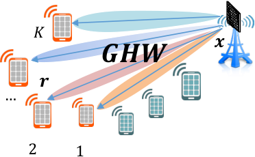
where are correspondingly transmitted and received vectors, is a downlink channel matrix, is a precoding matrix, and is a block-diagonal detection matrix; noise-vector is assumed to be independent Gaussian with noise level (Fig. 1). Note that the linear precoding and detection are implemented by simple matrix multiplications. The constant is the number of transmit antennas, is the total number of receive antennas, and is the total number of transmitted symbols in the system. They are usually related as . Each of the matrices decomposes by users: as it is shown on fig. 2, here are matrices correspond to UE .
2.1.1 Singular Value Decomposition of the Channel
It is convenient [21] to represent the channel matrix of UE via its reduced Singular Value Decomposition (SVD):
| (2) |
Where the channel matrix for user , contains channel vectors by rows, the singular values are sorted by descending, is a unitary matrix of left singular vectors, and matrix consists of right singular vectors vector-rows
Collecting all users together, we may write the following channel matrix decomposition: (Lemma 2.1 and Fig. 3), where each of the decomposition matrices consists of submatrices of which consist of vectors .
Lemma 2.1 (Main Decomposition).
For the linear system there exists a matrix expansion , Where — diagonal matrix of singular numbers, — matrix of general form, and the matrix — block-diagonal and unitary.
Note that this representation is not actually SVD-decomposition of the matrix : vectors that correspond to different UE are not generally orthogonal. Nonetheless, this representation has important properties that make it useful: the matrix is a diagonal matrix and is a block-diagonal unitary matrix. This allows to compensate factor by detection on UE side (each UE deals with its own ). Thus, on the transmitter side, it is sufficient to invert only the matrix , which in itself is much simpler than the channel : first, its rows have a unit norm and, second, it is a natural object for Rank adaptation problem [24]. We heavily use the Lemma 2.1 in the following.
2.1.2 Idea of Proposed Precoding Algorithm
Let us briefly formulate the resulting algorithm. The intuitive idea of the proposed precoding method is that it should provide maximum signal power and eliminate the so-called inter-user interference. It is known that maximal signal power is provided by Maximum Ratio Transmission (MRT) precoding, , and the interference is vanished by the Zero-Forcing (ZF) precoding, [3]. Both of these algorithms have disadvantages and can be improved by using Regularized Zero-Forcing (RZF) precoding , where the regularization parameter depends on noise level and average path-losses [4].
When users have significantly different path-losses, it is better to use regularization with a diagonal matrix. Non-scalar (matrix) regularization is introduced by E. Björnson in [5], where it is constructed using the primal-dual technique and demonstrated that the optimal regularization takes the shape of a diagonal matrix (generally speaking, with different elements). This proof is not constructive since it does not propose a specific formula or procedure for optimum regularization. In our work, we propose an explicit heuristic formula for diagonal regularization, Adaptive Regularized Zero-Forcing (ARZF) for the MU-MIMO system, as follows:
Theoretical justification is given below (Sec. 2.2). Experiments with Quadriga [9] show that proposed ARZF outperforms known scalar RZF algorithms (see Sec. 3.2).
2.1.3 Number of Transmitted Streams and Conjugate Detection
In the previous section, we have introduced the notation of SVD (eq. 2). Usually, the transmitter sends to UE several layers and the number of layers (rank) is less than the number of UE antennas (). In this case, it is natural to choose for transmission the first vectors from that correspond to the largest singular values from . Denote by the first largest singular values from , and by the first left and right singular vectors that correspond to :
| (3) |
where the wave sign denotes the contraction of singular vectors, i.e. . Numbers (and particular selection of ) are defined during the Rank Adaptation problem that, along with Scheduler, is solved before precoding. For the Rank adaptation problem, we refer for example to [24] and in what follows we consider , already chosen.
After precoding and transmission, on the UE side, we have to choose the detection matrix that takes into account UE Rank . The way, how UE performs detection, heavily affects the total performance and different detection algorithms require different optimal precodings (see [4] where precoding is a function of the detection matrix). The best way would be to choose precoding and detection consistently but it is hardly possible due to the distributed nature of wireless communication. Nevertheless, there are ideas on how to adjust the precoding matrix assuming a particular way of detection on the UE side at the transmitter [10]. We do not consider such an approach in this paper, though it can be used to further improve our main proposal.
To conduct analytical calculations, we assume the Conjugate Detection (CD) [25] in the following form:
| (4) |
where the unitary matrix contains the first singular vectors. The diagonal matrix contains the first of the largest singular values. A block-diagonal unitary matrix consists of blocks. The diagonal matrix consists of blocks . Finally, the block-diagonal detection matrix consists of the blocks on the main diagonal or, which is the same, the product of the matrices .
Theorem 2.2.
Conjugate Detection deletes unused singular vectors: , and the model equation (1) takes the form
| (5) |
Corollary 2.3.
Under the assumption of independent Gaussian noise the distribution of the effective noise vector (that appears with Conjugate Detection) is .
Proof.
| (7) |
∎
Remark 1.
The Corollary 2.3 is essential for our study, since it gives the idea to use in regularization part of precoding to take into account the correct effective noise .
Remark 2.
The formulated Theorem sufficiently simplifies the initial problem, decreases its dimensions, and allows notation to be uniform. Namely, we can work with user layers of shapes and instead of considering user antennas space. Note also that it is sufficient to only perform Partial SVD of the channel , keeping just the first singular values and vectors for each user such as
| (8) |
Based on this, in what follows we omit the tilde and write instead of correspondingly.
Remark 3.
The introduced Conjugate Detection is “ideal” and can not be implemented in practice. However, one can show that realistic detection policies as MMSE or IRC detection [26] often behave similarly to Conjugate Detection. In simulations, we use MMSE detection to compare various precoding methods.
2.1.4 Known MMSE Detection
Signal detection aims at pseudo-reversing the product of the channel and precoding matrices. The most common form of the detection matrix is studied, which are called minimum MSE (MMSE) [27]. In statistics and signal processing, MMSE — is an estimation method that minimizes the MSE function, which in turn is a general measure of the quality of the estimation of fitted values of the dependent variable.
The definition of MMSE detection implements the following rule:
| (9) |
The parameter — is the base station power, and — the system noise. The MMSE detection method seeks to eliminate noise by assuming it is the same for all symbols: , which may be violated in practice.
Lemma 2.4.
Proof.
Let’s substitute the system expression into the loss function .
The second summand will go to zero from introducing the expectation of noise with zero mean, and the third summand will go to zero
Let’s open the brackets using the sum norm squared formula:
| (10) |
Next, applying expectation over the symbols with the condition :
| (11) |
If the conditions are met: :
| (12) |
Let’s calculate the gradient of the function (12) and equate it to zero:
| (13) |
We get the desired solution (9).
∎
2.1.5 Quality Measures
The following functions are used to measure the quality of the precoding methods. These functions are based not on the actual sending symbols , but some distribution of them [5]. Thus, we get the common function for all assumed symbols, which can be sent using the specified precoding matrix.
Let us consider the end-to-end numbering of symbols for all UE and index function that returns the index of UE that receives the symbol . The Signal-to-Interference-and-Noise functional of the -th symbol of user is defined as:
| (14) |
The formula (14) shows the ratio between the useful and harmful parts of the signal. It depends on the whole precoding matrix , where the complex vector denotes the precoding for the -th symbol, on the channel matrix of the -th user, the detection vector of the -th symbol; after detection noise level of UE becomes . The formula (14) can be efficiently computed for all layers using several matrix multiplications and summations. It can be further simplified, using Theorem 2.2.
Corollary 2.5.
The important criterion of network performance is the spectral efficiency of UE , which refers to the information rate that can be transmitted over a given bandwidth for a certain UE. In the case of one symbol it is bounded by Shannon’s entropy that depends on SINR in the following way:
| (16) |
This is theoretically supreme for the possible transmission Rate, and recent modulation and coding schemes along with Hybrid Automatic Repeat Request (HARQ) retransmission and Block Error Rate (BLER) management allow us to achieve a Rate very close to Shannon’s entropy. Note that SINR here is taken in linear values, not in dB.
In the case of several transmitted symbols, generally speaking, of UE is not a sum over its layers because there is one common transport block to be transmitted and thus the coding and modulation algorithms are also common. Usually, one would introduce an effective SINR as a function of per-symbol SINR: , and so using (16) we obtain:
| (17) |
There are different approaches to estimate this effective SINR for QAM64 and QAM256 (see [28]) and in simulations, we use the QAM256 model. Also, we consider approximate formula using the geometric mean of per-symbol SINR. That is the same as the usual average of per-symbols in dB. This heuristic approximation will be used later in numerical optimization by gradient search:
| (18) |
The most general problem statement is the multi-criteria optimization of the whole vector . For such a problem, the Pareto optimality can be studied (see [29, 30]), which is hard and does not provide a unique solution, that is why usually a suitable decomposition into one-criterial optimization is considered: or [5]. Such decomposition can be done in different ways, we consider the sum of Spectral Efficiencies (17) over all UEs:
| (19) |
Such criterion is natural as UE Rates are additive values. There are other possible targets, e.g. performance of cell edge UE (CEU). In [12, sec. 7] interested readers can find Pareto analysis of the multi-criteria statement and comparison of several target functions, including
| (20) |
Finally, we consider Single-User SINR for the -th user and the average of SU SINR is an important parameter in simulations:
| (21) |
| (22) |
The formula (22) reflects the quality of the channel (geometrical average of per-symbol SINR) for the specified UE without taking into account other users. It depends on the greatest singular values of the -th user channel matrix and may be derived from the (14) and (18) formulas assuming Single-User case, MRT or ZF precoding matrix and Conjugate Detection (4). We will use this function in our experiments as a universal channel characteristic, including system noise and station power .
2.1.6 Problem Statement and Power Constraints
First of all, we assume that the total channel , the number of UE, and their ranks are known given values. This means that the Scheduler problem (which UE are to be served from the set of active UE) and Rank adaptation problem (which rank is provided to each UE) are already solved. This is usually the case in real networks. Scheduler and Rank adaptation problems are complicated and important radio resource management problems themselves but are out of the scope of this study (for example of Scheduler problem we refer to [31] and bibliography within, for Rank adaptation, [24] and [10]. These algorithms affect the properties of matrix , e.g. Scheduler can choose only UE with small enough correlations . We take this into account and consider scenarios with small correlations of UE channels.
Next, we consider the channel model in the form (1) that particularly means exact measurements of the channel. To further simplify the problem we suppose detection policy to be a known function, moreover we assume Conjugate Detection (4) that simplifies channel model to (5). Based on this channel model we calculate SINR of transmitted symbols by (15) and effective SINR of UE, which can be approximately calculated by (18).
Finally, denote the total power of the system as and that the sent vector has unit norm . The total power constraints and the more realistic per-antenna power constraints (see [12]) impose the following conditions on the precoding matrix:
| (23) |
The ultimate goal is to find a precoding matrix that maximizes sum Spectral Efficiency (17) subject to power constraints (23), e.g.:
| (24) |
Even after all the above simplifications, the formulated problem is too complicated to solve analytically. Moreover, it is not convex or concave, hence it could have a lot of (essentially) different local maximums. That’s why our strategy in this paper is to propose some heuristic formula that will prove to be better than known algorithms on some reliable simulations. After defining the particular form of precoding (anzats) we can always satisfy power constraints by normalizing constant, e.g. for (23):
| (25) |
In simulations, we use more realistic per-antenna power constraints.
2.2 Reference Precoding Methods
We repeat known reference precoding algorithms and present our solution.
2.2.1 Maximum Ratio Transmission (MRT)
A Maximum Ratio Transmission precoding algorithm takes single-user weights from the SVD-decomposition. This approach leads to the maximization of single-user power, ignoring the interference. The MRT approach is preferred in noisy systems when the noise power is higher than inter-user interference [3]:
| (27) |
where normalizing constant is defined from power constraint (25). This algorithm outputs a set of interfering channels assuming the model (5):
2.2.2 Zero-Forcing (ZF)
The next modification of the precoding algorithm performs decorrelation of the symbols using the inverse correlation matrix of the channel vectors. Such precoding construction sends the signal beams to the users without creating any interference between them. Different from the MRT method, the Zero-Forcing approach is preferred when the potential inter-user interference is higher than the noise power, and the Spectral Efficiency quality improves by eliminating this interference [3].
| (28) |
The following receiver model is:
Denote .
Theorem 2.6.
Assume the channel matrix has the form of (Lemma 2.1). Then, the following relation for Zero-Forcing holds:
| (29) |
Proof.
| (30) |
∎
2.2.3 Regularized Zero-Forcing (RZF)
In the geometrical sense, in the ZF method (28), beams are sent not directly to the users but with some deviation, which reduces the useful signal. The following modification corrects the beams, which allows some inter-user interference and significantly increases the payload.
In the practical sense, in the ZF method (28), the channel right inversion may not exist or matrix may be ill-conditioned, making ZF poorly perform. There are many practical solutions to this problem based on regularization.
| (31) |
Regularized Zero-Forcing is the most common method in real practice, and therefore we use it as the main reference method. As the baseline, we use the analytical form of the regularization matrix using [8].
This method cannot cancel all multi-user and multi-layer interference. It admits some interference to maximize single-user power. It is used as a trade-off between using MRT and ZF precoding [5] balancing between maximizing the signal power and minimizing the interference leakage, and thus we need to appropriately manage them by optimizing the regularization parameter depending on the noise level.
The RZF method has the following asymptotic properties [3]: if , it becomes equivalent to , which is optimal in low SINR cases. And if we set , the formula becomes equal to ZF precoding: , which is optimal in high SINR cases.
The precoding matrix based on the un-normalized channel [6] in the case when the number of sending symbols is less than the number of receiver antennas may be written in the following form of RZF:
| (32) |
Here, parameter and [8] are chosen taking into account noise level . Actually, this method is equivalent to an un-normalized channel matrix , which in our case is the matrix , obtained after splitting user channel into multiple streams.
Let us formulate the following well-known fact about RZF method (31).
Theorem 2.7.
Consider the channel decomposition from the Lemma 2.1. The precoding with any parameter is the solution of the following optimization problem:
| (33) |
Proof.
Calculating the gradient and equating it to zero, we get:
| (34) | ||||
The last identity may be proved using multiplication by the matrix from the right side of the identity and by the from the left side of it.
∎
Remark 4.
The algorithm is also the solution to the constrained optimization problem (26) in assumption (see [4]):
| (35) |
Constraint optimization problem (35) is decomposed to (33) with Lagrangian multiplier . In other words, is a special case of the Wiener filter [4, Eq. (34),(35)], when covariance matrices of signal and noise are and and at assumption of special detection .
2.2.4 Wiener Filter Zero-Forcing (WRZF)
In [4] authors study the Wiener filter that provides optimum in the problem (35) for arbitrary symbol and noise covariance matrices and in the case of known detection matrix . We take Conjugate Detection (4) and apply the Wiener filter for normalized channel and symbol and corresponding noise covariance . The algorithm
| (36) |
is the solution to the constrained optimization problem (26) in assumption of CD ( so that according to Theorem 2.2):
| (37) |
where .
2.3 Proposed Precoding Methods
2.3.1 Proposed Adaptive Regularized Zero-Forcing (ARZF)
Algorithms and (and even the Wiener filter in more general cases) are precodings with scalar Regularization. Taking into account effective noise from Corollary 2.3, we propose Adaptive RZF (ARZF) algorithm with diagonal matrix regularization:
| (38) |
ARZF allows the application of different regularization for different users and layers corresponding to their singular values that also include UE path loss.
Using , let’s write out the quadratic error of the received and sent symbols and :
| (39) |
Let’s introduce the inverse noise covariance matrix into the definition of norm, and we get the following weighted least squares function (40):
| (40) |
Theorem 2.8.
Proof.
Calculating the gradient and equating it to zero, we get:
| (42) |
The last identity may be proved using multiplication by the matrix from the right side of the identity and by the from the left side. ∎
Remark 5.
Optimization problem (41) is not common, and it can not be formulated in the form similar to (35). Nevertheless, such a problem statement is a more adequate approximation to sum SE maximization problem (24): because ARZF provides a larger sum SE than RZF of WRZF. Detailed simulation results are given below.
Remark 6.
The proposed algorithm along with Theorem 2.8 is the main result of the paper. Transmit Wiener Filter [4] algorithms have scalar regularization of the form , so ARZF is not from this class. As it is shown in [5], the maximum of the function of UE SINR (incl. considered the sum of SE (17)) is achieved by an algorithm with a proper diagonal regularization, and ARZF is a suboptimal heuristic of such form.
The possible interpretation of the function (33) is as follows. The second term is the standard noise regularization part and the first term, the norm , weighted by the matrix , weights more for the layers with higher singular values. And, therefore, the function is optimized more precisely for the layers with a higher signal quality compared to the layers with lower signal quality. In other words, precoding vectors for layers with higher singular values become similar to Zero-Forcing precoding, and for layers with lower singular values become similar to Maximum-Ratio Transmission, i.e. ARZF provides adaptive regularization. In the next section, we will see that this approach leads to a uniform increase in spectral efficiency compared to the basic method with unit weights.
Let us study the relation of ARZF with other algorithms. Firstly, we see that regularization parameter in WRZF is the (arithmetical) average of ARZF regularization:
In the case when path-losses of all UE are similar ARZF and WRZF provide a similar result. Secondly, the relation between and precoding is formulated as follows:
Theorem 2.9.
Assume the channel matrix has the form of (Lemma 2.1) and denote . Then, the following relation for ARZF holds:
| (43) |
Proof.
| (44) |
∎
Right factor in the r.h.s. of (43) can be interpreted as a special type of Power Allocation algorithm (see an interesting study in [12, sec. 7]) that distributes the total transmission power between layers. In practice, it is better to use rather than , because the norms of the rows of the matrix can differ sufficiently (up to several orders!), which leads to unbalanced power distribution between layers (as state Theorem 2.8 another way is to apply a proper Power allocation for . On the other hand, the regularization parameter of is more natural and correct. The proposed combines the benefits from these two approaches and provides an envelope of them.
Remark 7.
In this work we prove theoretical estimates of the number of conditionality of the inverse covariance matrix of the ARZF method and the standard RZF method, which is important for systems with fixed computational accuracy
Theorem 2.10.
Let , and given matrices and , that are inverted in the corresponding precodings , and . Then the conditioning numbers of and matrices are equal, respectively:
| (45) |
and are also related by the ratio:
- 1.
, if ,
- 2.
, if ,
where
Proof.
The assumption that the matrix of singular user vectors is close to unitary is valid under low correlation user selection: , with . Then the matrices under study are reduced to diagonal:
Their conditionality functions are equal (45).
By comparing these functions, we get transition points where it is clearly better to use the first formula : , it is better to use the second : . ∎
Remark 8.
In the situation nothing can be said and further investigation is required. Note that only case 1) is used in real networks. Singular vectors whose singular values are smaller than the noise power are not used, so the condition is always satisfied.
The mathematical notation improves the conditionality of the system under low to medium noise conditions, which makes the algorithm computationally more accurate under limited discharge grid conditions compared to another mathematical notation of the method . An experimental comparison of the conditionality value is shown in Fig. 4.
2.3.2 Asymptotic properties of ARZF
Using the Neumann series [33], we formulate the following
Lemma 2.11.
Consider square Hermit matrices and of the same size and full rank. Introduce a small parameter . The following and same size square matrices the following asymptotic holds:
| (46) |
where as .
Proof.
We are looking for the inverse in the form of formal series . Calculating product of and its inverse, we get the chain of equations for each power of :
| (47) | ||||||
| (48) |
∎
The following theorem 2.12 gives the asymptotic properties of ARZF.
Theorem 2.12.
Assume that matrix is of full rank equals to . It holds:
| (49) | ||||||
| (50) |
Proof.
Property at low noise is the same as for . Another asymptotic from Theorem 2.12 means that, when noise is greater than signal even for UE with the best channel, ARZF only serves UE with the best channel.
2.3.3 Gradient-Based Optimal Regularization (OPT)
Define detection function using (9);
Define target function of (14), (16), (19);
Set tolerance grad , termination tolerance on first order optimality (1e-5);
Set tolerance change , termination tolerance on function and parameters (1e-9);
Initialize regularization by ;
for to do
The proposed algorithm provides minimum to quadratic optimization problem (41), but still, there is a question: how good is it w.r.t. to sum SE function (19)? In [5] it is proved that optimal solution to the function with total power constraint is given by algorithm of the form
| (51) |
It is hardly possible to explicitly express the particular values of for optimal precoding but the structure itself is useful. According to this result, we are going to study the effectiveness of the proposed ARZF algorithm comparing it with gradient search over the sum of SE (17).
To this end we formulate an iterative solution with differentiable embedded parts. The proposed parametric solution preserves the structure of the basic RZF algorithm and optimizes the target functional of SE, which leads to a significant improvement in quality. We set the constrained smooth optimization problem. The problem is to find the local maximum of the Spectral Efficiency (19):
| (52) |
A parametric solution uses the RZF formula as follows:
| (53) | ||||
We restrict the maximum power of antennas by multiplying the precoding matrix by the scalar, which allows us to satisfy the power constraints and save the geometry and desired properties of the constructed precoding.
In further experiments, we will make the real diagonal matrix differentiable and optimize it for the target Spectral Efficiency functional, which is one of our contributions. The optimization of precoding matrix is given in the corresponding article [35].
Detection is involved in the calculation of the gradient, it can be considered as an integral part of the Spectral Efficiency. That is, the differentiable variables here are the diagonal of the regularization matrix, then the precoding matrix is calculated using the regularization, then this precoding is substituted into the detection. Finally, the calculated precoding and detection are both substituted into the gradient. The regularization diagonal is involved in all these operations as an internal variable of a composite function, and its gradient can be calculated using a chain rule, back-propagation algorithm, as it happens using automatic differentiation of the PyTorch library.
Remark 9.
In considered gradient optimization precoding is constructed, assuming some particular detection that could be performed on the UE side (namely, MMSE detection). This idea is widely discussed in state-of-the-art (see e.g. [10]) and can be used to improve merely any precoding policy with a corresponding iterative procedure.
3 Simulation Results and Discussion
3.1 Setup in Quadriga
In this section, we describe how we obtain data from Quadriga, open-source software for generating a realistic radio channel. The considered scenario is Urban Non-Line-of-Sight 3GPP_38.901_RMa_NLOS [23, 36].
Fig. 5 shows an example of user placement, and users are assigned either in a cluster of one of the buildings or on the ground next to a building. The users are highlighted with blue circles, and the base station — one in red. The distances between the individual antennas of the station and the users are negligible compared to the distances between the users and the station, so the station and users are depicted as separate circles, each containing multiple antennas within it.
The overall procedure is as follows, for each random seed:
- 1.
We generate a random environment around the base station;
- 2.
We select random user positions near the base station;
- 3.
We select relevant users based on correlations.
Next, we describe the procedure in detail.
First, we fix the position of the base station at the coordinates and set the random seed in Quadriga [9] to generate a random environment.
Second, we select the random user positions around the base station. To do this, we locate users in the urban landscape (see example at Fig 5):
- 1.
We sample up to 8 cluster centers , in the 120∘ sector from the base station within 2000m from the base station. Each cluster represents a part of a city building;
- 2.
We assign a random cluster height m , selecting the cluster floor in a building from the uniform distribution ;
- 3.
For each user, we assign a cluster id and sample position randomly over the 60m circle around the cluster centre;
- 4.
We sample the height of each user in addition to the height of the cluster, at the same time, 80% of users are placed near the cluster floor m. and 20% of users are placed outdoors m.
Third, after generating channel matrices for a fairly large number of users , we perform the user selection to choose subsets of users that will be served together (this procedure simulates Scheduler). We select one subset of users, such that there is no pair of too high correlated users (in real life users with high correlations are served at a different time or on different frequency intervals). The correlation between users is measured as the squared cosine between the main singular vectors: . The number of transmitted symbols for each UE is (it is the simplest Rank Selection policy).
We also consider two different situations (scenarios):
- 1.
When UE have different path-losses (PL), when we add random factor
, which is the realistic channel variance for close UE (in real networks path-loss variance for UE within one cell can be up to ). - 2.
When UE have almost equal path-losses, i.e. first singular values of each two UE are the same (this is the default option for Quadriga channel generation);
Presented results are the average over 40 considered random realizations of channel matrix and UE subsets. Namely, for each scenario we generate 40 different channels: :
- •
base station antennas;
- •
users;
- •
total user antennas;
- •
total user layers.
The carrier frequency for each channel matrix is selected randomly over the bandwidth. The base station antenna array forms a grid with placeholders along the axis and placeholders along the axis, the receiver antenna array consists of two placeholders along the . Each placeholder contains two cross-polarized antennas. Our user generation algorithm produces realistic setups for the Urban case and can be convenient for other studies. An interested reader can find detailed hyperparameters for antenna models and generation processes in Table 6 in Appendix.
3.2 Results and Discussion
We compare the proposed algorithm (ARZF) with reference algorithms (MR, ZF, RZF, WRZF) and the estimation of the precoding with optimal diagonal regularization (OPT). In Fig. 6 (Tab. 2) and Fig. 7 (Tab. 3) the Average Spectral Efficiency (19) and the Minimal SE (20) of the described algorithms are presented for the different path-loss scenarios. In Fig. 8 (Tab. 2) and Fig. 9 (Tab. 5) the same quality functions are compared for the equal path-loss scenario.
ARZF (the red line, 38) provides the best Average Spectral Efficiency (19) compared to all other analytical methods up to the highest SUSINR region (see Fig. 6, 8). The advantages of the ARZF algorithm are revealed due to adaptive regularization for a specific path-loss (and thus singular values order) for each user. In detail, the situation is as follows. ZF ( and ) are better than MRT () on high SUSINR region, and are worse for low SUSINR ( is always better than ). RZF is better than both MRT and corresponding ZF, e.g. is better than and . One can say that RZF provides an envelope of MRT and ZF. It is worth saying that although outperforms on high SUSINR region is better for low SUSINR. Due to the adaptive approach, ARZF makes an envelope of both RZF algorithms. It is quite natural that on equal path-loss scenario, WRZF and ARZF work similarly: it happens because all the singular values are almost the same. Well, on the different path-loss scenarios, WRZF degrades significantly and ARZF is better.
One may notice, that the gradient-based iterative method OPT (the black line, (1)) provides superior results. On the other hand, OPT is computationally expensive and cannot be used in practice. However, OPT is very good for upper bound estimation: the results for OPT show that the ARZF method can be improved in further research. We also measure the quality of Minimal Spectral Efficiency (20) (see Fig. 7, 9) to investigate the performance of the weakest user.
These results show that the ARZF method, configuring the regularization in a special adaptive way, outperforms the Average SE at the expense of Minimal SE, i.e. of the weaker users. This follows from the fact that in terms of the Minimal SE function, the ARZF method can lose compared to other algorithms, especially in the low SUSINR region. The Average SE quality of the system, however, increases significantly. The contradiction between Average and Minimal SE functions is well-known (see. e.g. [12]).
Fig. 8 (Tab. 4) and Fig. 9 (Tab. 5) represent Average and Minimal scenarios and show the experimental results for users with almost equal path-losses. The general tendency is the same as for different path-loss scenarios: The proposed ARZF method outperforms all other analytical references in the Average SE, but it is not the best from the Minimal SE point of view. In this scenario the gain in Average SE is not so big, particularly, ARZF behaves almost the same way as WRZF. The last observation in Fig (8) (Tab. (4)) is very important. The red line of coincides with the blue line of . This result shows that both algorithms work the same when users have equal path-losses, which is also confirmed by theoretical calculations
4 Conclusions
Multi-user precoding optimization is a key problem in modern cellular wireless systems, which are based on massive MIMO technology. In this paper, we analyze the performance of different transmission precoding techniques in a downlink multi-user scenario. Linear techniques are computationally less expensive. On the other hand, non-linear techniques can provide better performance. The first technique that we propose in this paper is a low-complexity heuristic formula of the Adaptive Regularized Zero-Forcing (ARZF) algorithm. This technique is especially attractive in cases when the users and the base station are equipped with multiple antennas and have various path losses. We study analytically the relation of ARZF with known RZF-like algorithms and its asymptotic properties. Finally, we study the properties of the proposed ARZF method on simulations, using a realistic Quadriga channel. Simulations show uniform improvement over the reference methods to Average Spectral Efficiency for all considered scenarios. This particularly means that weighted MSE problem statement (41) is a more adequate approximation of (24) than the standard MMSE statement. Minimal Spectral Efficiency function is not the best, but is still acceptable over ARZF. We also introduce a non-linear technique Gradient-Based Optimal Regularization (OPT) that performs gradient optimization on the target Spectral Efficiency function and finds the optimal diagonal regularization matrix this way. This algorithm can be used for the upper bound study.
Declarations
4.1 Availability of data and materials
The Quadriga-generated channel matrices, as well as the full Python implementation of the proposed approach and baselines, are publicly available in the Github repository at https://github.com/eugenbobrov/Adaptive-Regularized-Zero-Forcing-Beamforming-in-Massive-MIMO-with-Multi-Antenna-Users
4.2 Authors Contribution
EB and BC formulated the proposed formula of ARZF; EB, BC, DM and DY formulated, proved, and wrote the theoretical results section; EB did the main work of conducting the experiments and drafting the manuscript; BC also did the main work of the literature review and the introduction; EB and DM conceived the study; ST helped with dataset preparation; VK and DM were involved in methodology; HL and DZ contributed to project administration and supervision. All authors read and approved the final manuscript.
4.3 Acknowledges
Authors are grateful to E. Barinova and E. Levitskaya for support.
4.4 Funding
Authors have received research support from Huawei Technologies.
4.5 Competing Interest
The authors declare that they have no competing interests.
| Precoding | ||||||||
|---|---|---|---|---|---|---|---|---|
| SU SINR | ||||||||
| 0 | 1.45 | 2.27 | 0.02 | 2.37 | 2.46 | 1.48 | 3.91 | 4.07 |
| 4 | 1.75 | 3.13 | 0.05 | 3.19 | 2.79 | 1.84 | 4.91 | 5.10 |
| 8 | 2.08 | 4.16 | 0.11 | 4.19 | 3.10 | 2.33 | 6.03 | 6.32 |
| 12 | 2.41 | 5.29 | 0.26 | 5.31 | 3.37 | 3.02 | 7.17 | 7.63 |
| 16 | 2.71 | 6.51 | 0.54 | 6.52 | 3.61 | 4.02 | 8.23 | 9.01 |
| 20 | 2.99 | 7.79 | 1.03 | 7.79 | 3.66 | 5.48 | 9.26 | 10.42 |
| 24 | 3.24 | 9.05 | 1.75 | 9.05 | 3.76 | 7.29 | 10.23 | 11.74 |
| 28 | 3.47 | 10.40 | 2.77 | 10.40 | 4.08 | 9.58 | 11.24 | 13.09 |
| 32 | 3.65 | 11.65 | 3.95 | 11.65 | 4.73 | 11.60 | 12.19 | 14.17 |
| 36 | 3.76 | 12.83 | 5.16 | 12.83 | 5.55 | 13.10 | 13.13 | 15.24 |
| 40 | 3.83 | 13.90 | 6.34 | 13.90 | 6.52 | 14.21 | 14.05 | 16.17 |
| Precoding | ||||||||
|---|---|---|---|---|---|---|---|---|
| SU SINR | ||||||||
| 0 | 0.02 | 0.01 | 0.02 | 0.01 | 0.00 | 0.02 | 0.00 | 0.00 |
| 4 | 0.05 | 0.02 | 0.04 | 0.02 | 0.01 | 0.05 | 0.00 | 0.00 |
| 8 | 0.12 | 0.04 | 0.10 | 0.04 | 0.06 | 0.13 | 0.00 | 0.00 |
| 12 | 0.28 | 0.11 | 0.19 | 0.11 | 0.21 | 0.29 | 0.02 | 0.03 |
| 16 | 0.57 | 0.26 | 0.34 | 0.26 | 0.59 | 0.56 | 0.08 | 0.11 |
| 20 | 1.04 | 0.58 | 0.54 | 0.58 | 1.12 | 1.01 | 0.28 | 0.23 |
| 24 | 1.62 | 1.16 | 0.76 | 1.16 | 1.46 | 1.67 | 0.75 | 0.52 |
| 28 | 2.24 | 2.19 | 0.99 | 2.19 | 1.56 | 2.68 | 1.74 | 0.89 |
| 32 | 2.67 | 3.67 | 1.18 | 3.67 | 1.47 | 4.05 | 3.34 | 1.63 |
| 36 | 2.89 | 5.45 | 1.34 | 5.45 | 1.47 | 5.70 | 5.29 | 2.74 |
| 40 | 3.00 | 7.52 | 1.47 | 7.52 | 1.51 | 7.67 | 7.49 | 4.25 |
| Precoding | ||||||||
|---|---|---|---|---|---|---|---|---|
| SUSINR | ||||||||
| 0 | 1.00 | 0.54 | 0.25 | 0.96 | 1.19 | 1.12 | 1.19 | 1.39 |
| 4 | 1.60 | 1.11 | 0.57 | 1.56 | 1.86 | 1.92 | 1.99 | 2.26 |
| 8 | 2.25 | 2.08 | 1.23 | 2.46 | 2.71 | 3.03 | 3.09 | 3.49 |
| 12 | 2.85 | 3.54 | 2.40 | 3.81 | 3.81 | 4.46 | 4.47 | 5.03 |
| 16 | 3.30 | 5.41 | 4.09 | 5.57 | 5.12 | 6.14 | 6.12 | 6.86 |
| 20 | 3.57 | 7.52 | 6.11 | 7.60 | 6.73 | 8.00 | 7.99 | 8.83 |
| 24 | 3.73 | 9.64 | 8.23 | 9.69 | 8.56 | 9.94 | 9.90 | 10.83 |
| 28 | 3.81 | 11.56 | 10.19 | 11.59 | 10.36 | 11.73 | 11.70 | 12.74 |
| 32 | 3.85 | 13.29 | 11.99 | 13.31 | 12.07 | 13.38 | 13.36 | 14.59 |
| 36 | 3.87 | 14.57 | 13.34 | 14.58 | 13.38 | 14.62 | 14.60 | 16.02 |
| 40 | 3.88 | 15.50 | 14.36 | 15.51 | 14.38 | 15.53 | 15.52 | 17.15 |
| Precoding | ||||||||
|---|---|---|---|---|---|---|---|---|
| SUSINR | ||||||||
| 0 | 0.42 | 0.16 | 0.24 | 0.33 | 0.33 | 0.45 | 0.09 | 0.11 |
| 4 | 0.85 | 0.38 | 0.56 | 0.60 | 0.83 | 0.91 | 0.30 | 0.33 |
| 8 | 1.48 | 0.86 | 1.21 | 1.08 | 1.71 | 1.60 | 0.83 | 0.91 |
| 12 | 2.18 | 1.77 | 2.36 | 1.96 | 3.05 | 2.58 | 1.85 | 1.89 |
| 16 | 2.67 | 3.22 | 4.00 | 3.34 | 4.70 | 3.88 | 3.40 | 3.35 |
| 20 | 2.90 | 5.12 | 5.86 | 5.19 | 6.51 | 5.55 | 5.34 | 5.33 |
| 24 | 2.99 | 7.25 | 7.67 | 7.28 | 8.07 | 7.49 | 7.41 | 7.38 |
| 28 | 3.02 | 9.19 | 9.16 | 9.21 | 9.35 | 9.33 | 9.30 | 9.67 |
| 32 | 3.04 | 10.84 | 10.31 | 10.85 | 10.40 | 10.92 | 10.91 | 11.54 |
| 36 | 3.04 | 11.93 | 11.02 | 11.93 | 11.06 | 11.97 | 11.96 | 12.83 |
| 40 | 3.05 | 12.61 | 11.44 | 12.62 | 11.45 | 12.63 | 12.63 | 13.74 |
| Parameter | Value |
| Base station parameters | |
| number of base stations | |
| position, m: (x, y, z) axes | |
| number of antenna placeholders (y axis) | |
| number of antenna placeholders (z axis) | |
| distance between placeholders ( axis) | wavelength |
| distance between placeholders ( axis) | wavelength |
| antenna model | 3gpp-macro |
| half-Power in azimuth direction, deg | 60 |
| half-Power in elevation direction, deg | 10 |
| front-to back ratio, dB | 20 |
| total number of antennas | 64 |
| Receiver parameters | |
| number of placeholders at the receiver ( axis) | |
| distance between placeholders ( axis) | wavelength |
| antenna model | half-wave-dipole |
| total number of antennas | 4 |
| Quadriga simulation parameters | |
| central band frequency | GHz |
| 1 sample per meter (default value) | 1 |
| include delay of the LOS path | 1 |
| disable spherical waves (use_3GPP_baseline) | 1 |
| Quadriga channel builders parameters | |
| shadow fading sigma | 0 |
| cluster splitting | False |
| bandwidth | MHz |
| number of subcarriers | 42 |
Abbreviations
| MIMO | Multiple-input multiple-output |
| ZF | Zero-Forcing |
| RZF | Regularized Zero-Forcing |
| MRT | Maximum Ratio Transmission |
| DPC | Dirty Paper Coding |
| UE | User equipment |
| CEU | Cell Edge User equipment |
| RSRP | Reference Signal Received Power |
| VP | Vector Perturbation |
| CD | Conjugate Detection |
| SINR | Signal-to-Interference-and-Noise |
| HARQ | Hybrid Automatic Repeat Request |
| BLER | Block Error Rate |
| SE | Spectral Efficiency |
| MSE | Mean Squared Error |
| MMSE | Minimum Mean Squared Error |
| WRZF | Wiener Filter Zero-Forcing |
| ARZF | Adaptive Regularized Zero-Forcing |
| OPT | Gradient-Based Optimal Regularization |
| LOS | Line-of-Sight |
| NLOS | Non-Line-of-Sight |
| SVD | Singular Value Decomposition |
| CSI | Channel state information |
| TDD | Time division duplex |
References
- [1] Hien Quoc Ngo, Erik G Larsson, and Thomas L Marzetta. Energy and spectral efficiency of very large multiuser MIMO systems. IEEE Transactions on Communications, 61(4):1436–1449, 2013.
- [2] Jeffrey G Andrews, Stefano Buzzi, Wan Choi, Stephen V Hanly, Angel Lozano, Anthony CK Soong, and Jianzhong Charlie Zhang. What will 5G be? IEEE Journal on selected areas in communications, 32(6):1065–1082, 2014.
- [3] Tebe Parfait, Yujun Kuang, and Kponyo Jerry. Performance analysis and comparison of ZF and MRT based downlink massive MIMO systems. In 2014 sixth international conference on ubiquitous and future networks (ICUFN), pages 383–388. IEEE, 2014.
- [4] Michael Joham, Wolfgang Utschick, and Josef A Nossek. Linear transmit processing in MIMO communications systems. IEEE Transactions on signal Processing, 53(8):2700–2712, 2005.
- [5] Emil Björnson, Mats Bengtsson, and Björn Ottersten. Optimal multiuser transmit beamforming: A difficult problem with a simple solution structure [lecture notes]. IEEE Signal Processing Magazine, 31(4):142–148, 2014.
- [6] Long D Nguyen, Hoang Duong Tuan, Trung Q Duong, and H Vincent Poor. Multi-user regularized zero-forcing beamforming. IEEE Transactions on Signal Processing, 67(11):2839–2853, 2019.
- [7] Jiankang Zhang, Sheng Chen, Robert G Maunder, Rong Zhang, and Lajos Hanzo. Regularized zero-forcing precoding-aided adaptive coding and modulation for large-scale antenna array-based air-to-air communications. IEEE Journal on Selected Areas in Communications, 36(9):2087–2103, 2018.
- [8] Christian B Peel, Bertrand M Hochwald, and A Lee Swindlehurst. A vector-perturbation technique for near-capacity multiantenna multiuser communication-part i: channel inversion and regularization. IEEE Transactions on Communications, 53(1):195–202, 2005.
- [9] Stephan Jaeckel, Leszek Raschkowski, Kai Börner, and Lars Thiele. QuaDRiGa: A 3-D multi-cell channel model with time evolution for enabling virtual field trials. IEEE Transactions on Antennas and Propagation, 62(6):3242–3256, 2014.
- [10] Shuying Shi, Martin Schubert, and Holger Boche. Downlink MMSE transceiver optimization for multiuser MIMO systems: Duality and sum-MSE minimization. IEEE Transactions on Signal Processing, 55(11):5436–5446, 2007.
- [11] Giuseppe Caire and Shlomo Shamai. On the achievable throughput of a multiantenna Gaussian broadcast channel. IEEE Transactions on Information Theory, 49(7):1691–1706, 2003.
- [12] Emil Björnson, Jakob Hoydis, and Luca Sanguinetti. Massive MIMO networks: Spectral, energy, and hardware efficiency. Foundations and Trends in Signal Processing, 11(3-4):154–655, 2017.
- [13] Le-Nam Tran, Markku Juntti, Mats Bengtsson, and Bjorn Ottersten. Beamformer designs for MISO broadcast channels with zero-forcing dirty paper coding. IEEE transactions on wireless communications, 12(3):1173–1185, 2013.
- [14] Nusrat Fatema, Guang Hua, Yong Xiang, Dezhong Peng, and Iynkaran Natgunanathan. Massive MIMO linear precoding: A survey. IEEE systems journal, 12(4):3920–3931, 2017.
- [15] Kan Zheng, Long Zhao, Jie Mei, Bin Shao, Wei Xiang, and Lajos Hanzo. Survey of large-scale MIMO systems. IEEE Communications Surveys & Tutorials, 17(3):1738–1760, 2015.
- [16] Sunil Dhakal. High rate signal processing schemes for correlated channels in 5G networks. 2019.
- [17] Tadilo Endeshaw Bogale and Luc Vandendorpe. Sum MSE optimization for downlink multiuser MIMO systems with per antenna power constraint: Downlink-uplink duality approach. In 2011 IEEE 22nd International Symposium on Personal, Indoor and Mobile Radio Communications, pages 2035–2039. IEEE, 2011.
- [18] Ami Wiesel, Yonina C Eldar, and Shlomo Shamai. Zero-forcing precoding and generalized inverses. IEEE Transactions on Signal Processing, 56(9):4409–4418, 2008.
- [19] Jakob Hoydis, Stephan Ten Brink, and Mérouane Debbah. Massive MIMO in the UL/DL of cellular networks: How many antennas do we need? IEEE Journal on selected Areas in Communications, 31(2):160–171, 2013.
- [20] Emil Björnson, Eduard Jorswieck, and Bjorn Ottersten. Impact of spatial correlation and precoding design in OSTBC MIMO systems. IEEE Transactions on Wireless Communications, 9(11):3578–3589, 2010.
- [21] Liang Sun and Matthew R McKay. Eigen-based transceivers for the MIMO broadcast channel with semi-orthogonal user selection. IEEE Transactions on Signal Processing, 58(10):5246–5261, 2010.
- [22] Duy HN Nguyen and Tho Le-Ngoc. MMSE precoding for multiuser MISO downlink transmission with non-homogeneous user SNR conditions. EURASIP Journal on Advances in Signal Processing, 2014(1):1–12, 2014.
- [23] David Tse and Pramod Viswanath. Fundamentals of wireless communication. Cambridge university press, 2005.
- [24] Nurul H Mahmood, Gilberto Berardinelli, Fernando ML Tavares, Mads Lauridsen, Preben Mogensen, and Kari Pajukoski. An efficient rank adaptation algorithm for cellular MIMO systems with IRC receivers. In 2014 IEEE 79th Vehicular Technology Conference (VTC Spring), pages 1–5. IEEE, 2014.
- [25] Evgeny Bobrov, Boris Chinyaev, Viktor Kuznetsov, Dmitrii Minenkov, and Daniil Yudakov. Power allocation algorithms for massive mimo systems with multi-antenna users. Wireless Networks, pages 1–22, 2023.
- [26] Bin Ren, Yingmin Wang, Shaohui Sun, Yawen Zhang, Xiaoming Dai, and Kai Niu. Low-complexity MMSE-IRC algorithm for uplink massive MIMO systems. Electronics Letters, 53(14):972–974, 2017.
- [27] Ahmed Hesham Mehana and Aria Nosratinia. Diversity of mmse mimo receivers. IEEE Transactions on information theory, 58(11):6788–6805, 2012.
- [28] Sandra Lagen, Kevin Wanuga, Hussain Elkotby, Sanjay Goyal, Natale Patriciello, and Lorenza Giupponi. New radio physical layer abstraction for system-level simulations of 5G networks. In ICC 2020-2020 IEEE International Conference on Communications (ICC), pages 1–7. IEEE, 2020.
- [29] Harold W Kuhn and Albert W Tucker. Nonlinear programming. In Traces and emergence of nonlinear programming, pages 247–258. Springer, 2014.
- [30] Tjalling Koopmans. Activity analysis of production and allocation. 1951.
- [31] Le-Nam Tran. An iterative precoder design for successive zero-forcing precoded systems. IEEE communications letters, 16(1):16–18, 2011.
- [32] Karl Pearson. LIII. on lines and planes of closest fit to systems of points in space. The London, Edinburgh, and Dublin philosophical magazine and journal of science, 2(11):559–572, 1901.
- [33] Dengkui Zhu, Boyu Li, and Ping Liang. On the matrix inversion approximation based on neumann series in massive mimo systems. In 2015 IEEE international conference on communications (ICC), pages 1763–1769. IEEE, 2015.
- [34] Dong C Liu and Jorge Nocedal. On the limited memory BFGS method for large scale optimization. Mathematical programming, 45(1):503–528, 1989.
- [35] Evgeny Bobrov, Dmitry Kropotov, Sergey Troshin, and Danila Zaev. Finding better precoding in massive MIMO using optimization approach, 2021.
- [36] Frode Bohagen, Pål Orten, and GE Oien. Construction and capacity analysis of high-rank line-of-sight MIMO channels. In IEEE Wireless Communications and Networking Conference, 2005, volume 1, pages 432–437. IEEE, 2005.