The Relevance of Electronic Perturbations in the Warm Dense Electron Gas
Abstract
Warm dense matter (WDM) has emerged as one of the frontiers of both experimental and theoretical physics and is challenging traditional concepts of plasma, atomic, and condensed-matter physics. While it has become common practice to model correlated electrons in WDM within the framework of Kohn-Sham density functional theory, quantitative benchmarks of exchange-correlation (XC) functionals under WDM conditions are yet incomplete. Here, we present the first assessment of common XC functionals against exact path-integral Monte Carlo calculations of the harmonically perturbed thermal electron gas. This system is directly related to the numerical modeling of X-Ray scattering experiments on warm dense samples. Our assessment yields the parameter space where common XC functionals are applicable. More importantly, we pinpoint where the tested XC functionals fail when perturbations on the electronic structure are imposed. We indicate the lack of XC functionals that take into account the needs of WDM physics in terms of perturbed electronic structures.
I Introduction
Understanding transient states in warm dense matter (WDM) is one of the grand challenges of plasma physics that is currently being tackled in a number of experimental facilities Moses et al. 2009; Tschentscher et al. 2017; MacDonald et al. 2021; Ren et al. 2018. In these experiments, WDM is generated, for example, due to laser-induced shock compression Fortov et al. 2006; Graziani et al. 2014; Falk 2018. At the foundational level, probing WDM facilitates a better understanding of astrophysical objects such as planetary interiors Alfè, Gillan, and Price 1999; Nguyen and Holmes 2004; Militzer et al. 2008; Schöttler and Redmer 2018; Nettelmann et al. 2011; Kramm et al. 2012 and stars Chabrier et al. 2000; Saumon et al. 1992; Daligault and Gupta 2009; Haensel, Potekhin, and Yakovlev 2006. Furthermore, understanding WDM has great technological potential as it occurs during the fuel compression processes in inertial confinement fusion Hu et al. 2011. Finally, exploring novel materials properties by driving matter through the WDM regime is an active area of research Skiff and Wurtele 2017; Tamblyn, Raty, and Bonev 2008; Brongersma, Halas, and Nordlander 2015; Kandyla, Shih, and Mazur 2007.
The interpretation of WDM experiments relies on a strong interplay with theory and simulation, because typical parameters like density and temperature cannot be inferred solely from the experimental data. The use of quantum Monte Carlo (QMC) techniques has recently paved the way for determining the exact properties of interacting electrons in the uniform electrons gas under WDM conditions Dornheim, Groth, and Bonitz 2018a; Dornheim et al. 2019a; Dornheim et al. 2018a; Dornheim et al. 2018b; Dornheim, Vorberger, and Bonitz 2020a. However, this method is computationally expensive and does not take into account the coupling of the electrons to the ions explicitly. Kohn-Sham density functional theory (KS-DFT)Kohn and Sham 1965 has therefore emerged as the standard method to model the electronic structure in WDM, because it includes both electron-electron and electron-ion interactions. Due to its balance of accuracy and computational efficiency Pribram-Jones, Gross, and Burke 2015, KS-DFT enables calculating materials properties such as structural and electronic transport properties under the conditions relevant to the WDM community Desjarlais, Kress, and Collins 2002a; Desjarlais 2003; Mazevet et al. 2005a; Holst, Redmer, and Desjarlais 2008; Lorenzen, Holst, and Redmer 2009; Knudson et al. 2012; Knudson et al. 2015.
Here, the central quantity is the KS potential – a mean-field potential that mimics the electron-electron interaction, in principle, exactly. The key ingredient to the KS potential is the exchange-correlation (XC) functional. In practice, the XC functional needs to be approximated. From a historical perspective, the development of XC approximations has focused on the electronic structure of molecules and solids under ambient conditions Burke 2012. These are commonly ranked in terms of increasing accuracy and computational cost on the so-called Jacob’s ladder Perdew and Schmidt 2001. Starting at the lowest rung with the local density approximation (LDA) Kohn and Sham 1965, an array of XC approximations has been developed including, for instance, the generalized gradient approximation (GGA) Becke 1988; Perdew, Burke, and Ernzerhof 1996, the meta-GGA Tao et al. 2003; Sun, Ruzsinszky, and Perdew 2015, and hybrid functionals Becke 1993; Perdew, Ernzerhof, and Burke 1996; Heyd, Scuseria, and Ernzerhof 2003. A key step most relevant for WDM modeling is the generalization of KS-DFT to finite temperature Mermin 1965. Based on this, several works have fleshed out the theoretical aspects of functional construction at finite temperature Pittalis et al. 2011; Dufty and Trickey 2011; Burke et al. 2016; Pribram-Jones and Burke 2016. Most recently, these have led to the construction of XC functionals that have an explicit temperature dependence Karasiev, Sjostrom, and Trickey 2012; Karasiev et al. 2014; Karasiev et al. 2013; Sjostrom and Daligault 2013; Groth et al. 2017; Mihaylov, Karasiev, and Hu 2020.
Despite these efforts, functional development has not taken into account the needs of WDM physics to a large extent beyond the inclusion of finite-temperature effects in the electronic structure Karasiev, Calderin, and Trickey 2016; Zhang et al. 2021. Some exact conditions imposed for chemistry and solid-state physics are not relevant to WDM. For example, in contrast to solid-state physics, the surface energy has no significance in WDM, because the generated samples have no well defined surface, but rather transition to a plasma state Olson et al. 2004; Saunders et al. 2018; Reinholz et al. 2003. Conversely, there are properties that are highly important in WDM, but have little value for solid-state physics. The most prominent example are perturbations imposed on the electronic structure with respect to the wave number . An accurate description of such perturbations across a large range of is essential for WDM modeling. Accuracy is not only required in the long wavelength regime which is dominated by collective electronic excitations, but also at large wave numbers where so-called single-particle effects become important Hamann et al. 2020a; Hamann et al. 2020b; Moldabekov, Bonitz, and Ramazanov 2018; Moldabekov et al. 2015. Achieving a high accuracy on a wide range of wave numbers is essential, e.g., for modeling X-Ray Thomson scattering (XRTS) experiments, which is a technique of paramount importance in WDM diagnostics Glenzer et al. 2003.
In this paper, we therefore analyze the accuracy of common XC functionals in the WDM regime when perturbations on the electronic structure are imposed across a large range of wave numbers . To that end, we benchmark the results of KS-DFT calculations against path-integral QMC data which are considered exact within the given error bars. Specifically, we employ four common XC functionals the LDA in the Perdew-Zunger parametrization Perdew and Zunger 1981, the GGAs PBE Perdew, Burke, and Ernzerhof 1996 and PBEsol Perdew et al. 2008, and the meta-GGA SCAN Sun, Ruzsinszky, and Perdew 2015. We focus on the sensitivity of these XC functionals towards a perturbed electronic structure at a finite wave number . Thereby, we uncover failures of these XC approximations. Our result strongly highlights the need for novel XC functionals that remain accurate under a perturbed electronic structure that is typically present in WDM. Furthermore, to our knowledge, this assessment of KS-DFT against QMC data with respect to electronic density perturbations in the WDM regime has not been performed yet. While recent developments introduced above have addressed the explicit temperature dependence of XC functionals, they do not account for the physics that stems from perturbations at finite . In our analysis, we therefore separate the influence of finite temperature in the electronic states from the effect of perturbations in . We follow the common practice of using the listed ground-state XC approximations and including only the implicit temperature dependence of the electronic structure in terms of a Fermi-Dirac occupation of the KS states.
The paper is organized as follows: we introduce the theoretical aspects and the simulation methods in Section II; we present our results on benchmarking common XC approximations in Section III; we address the issue of finite size effects in Section IV; we assess the performance of the aforementioned XC functionals in terms of the total energy in Section V; we provide conclusions and an outlook on future perspectives in Section VI. We provide methodological details on KS-DFT and path-integral Monte Carlo (PIMC) in the Appendix.
II Theory and Simulation Methods
We begin our assessment with the following Hamiltonian that imposes electronic perturbations on a warm dense uniform electron gas (UEG):
| (1) |
where denotes the standard Hamiltonian of the UEG Loos and Gill 2016; Giuliani and Vignale 2008; Dornheim, Groth, and Bonitz 2018b, the number of electrons, the number of external harmonic perturbations, their amplitude, and the wave vector of the perturbations. In this work, we consider both one harmonic perturbation and the combination of two harmonic perturbations . Note that we work within atomic units throughout.
It has been shown that the electronic states described by Eq. (1) are generated in WDM experiments Dornheim, Vorberger, and Bonitz 2020b. Furthermore, Eq. (1) has been used to rigorously examine various fundamental physical properties of the electronic structure in WDM, such as the local field correction (LFC) Moroni, Ceperley, and Senatore 1995; Moroni, Ceperley, and Senatore 1992; Dornheim et al. 2017; Groth, Dornheim, and Bonitz 2017 and the non-linear response Dornheim, Vorberger, and Bonitz 2020b; Dornheim et al. 2020; Dornheim et al. 2021 that are used to describe XRTS signals. Moreover, it turns out that the UEG model provides an excellent description of many electronic properties in WDM, because the electron-ion coupling can be relatively weak Dornheim et al. 2020; Clérouin et al. 2015; Grabowski et al. 2020.
The Hamiltonian in Eq. (1) is a convenient device to control the degree of inhomogeneity and the wave number of the imposed perturbations on the UEG by tuning the parameters and , respectively. We analyze the performance of XC functionals with respect to electronic density perturbations by considering an amplitude range . This range covers regimes from weak density perturbations with to strongly inhomogeneous electronic systems with , where . Additionally, we consider perturbations imposed by tuning the wave number in the range . Thereby, we assess the performance of XC functionals at different length scales ranging from the long wavelength regime defined by collective behavior Hamann et al. 2020a; Hamann et al. 2020b to the scale defined by the single-particle limit Moldabekov, Bonitz, and Ramazanov 2018; Dornheim et al. 2019a. This covers the entire range of wave numbers relevant to WDM generated in experiments.
WDM conditions prevail when we consider matter at solid density and a temperature Bonitz et al. 2008; Moldabekov et al. 2018, where denotes the Fermi temperature defined in terms of the Fermi energy and the Boltzmann constant . In our analysis, we consider the densities and and a temperature , where defines the number density of electrons which is given as the ratio between the Wigner-Seitz radius and the first Bohr radius . At , the parameter also characterizes electronic non-ideality Ott, Torben et al. 2018; Moldabekov, Dornheim, and Bonitz 2021. Therefore, it is used also as a coupling parameter. These parameters are typically encountered in experiments with laser-driven and shock-compressed solid targets Landen et al. 2001; Glenzer et al. 2007; Ciricosta et al. 2012.
The KS-DFT calculations were performed with the GPAW code Mortensen, Hansen, and Jacobsen 2005; Enkovaara et al. 2010; Larsen et al. 2017; Bahn and Jacobsen 2002, which is a real-space implementation of the projector augmented-wave method. Details of the KS-DFT simulation parameters such as the number of -points and number of bands are given in the Appendix.
We provide unassailable data for benchmarking our KS-DFT results by carrying out direct path-integral QMC calculations based on Eq. (1) without any restrictions on the nodal structure of the thermal density matrix. Therefore, the calculations are computationally expensive due to the fermion sign problem Dornheim 2019; Dornheim 2021, but exact within the given Monte Carlo error bars. The corresponding simulation details, such as the number of imaginary-time propagators, can be found in the Appendix Appendix: PIMC simulation details.


III Results
III.1 Single Harmonic Perturbation
Let us begin our analysis by considering the case of a single harmonic perturbation, i.e., in Eq. (1). First, we investigate the electronic density distribution at a density (coupling) parameter for a range of perturbation amplitudes and wave numbers. Then, we consider a stronger coupling regime at . These parameters are of particular interest in WDM experiments.
III.1.1 Metallic Density,
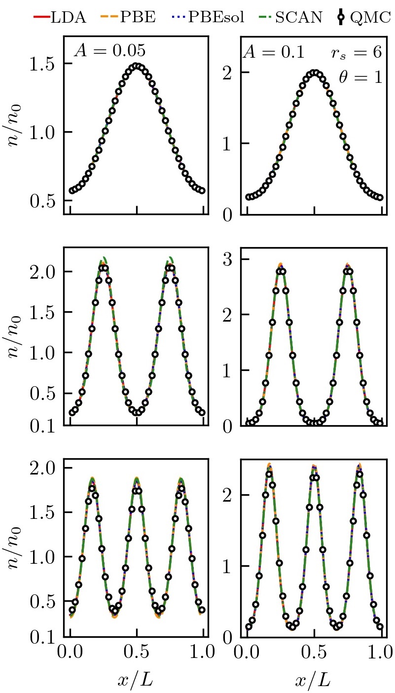
The density distribution along the direction of the density perturbation is shown for two amplitudes and and increasing wave number in Fig. 1. The top panel displays the results for , the middle panel for , and the bottom panel for . On the scale of the total density, all considered XC functionals are in overall agreement with each other and with the QMC data.
Let us now consider the actual deviation of the KS-DFT data from the reference QMC data in closer detail. To that end, we consider the relative density deviation between the KS-DFT data and the reference QMC data, where is the maximum deviation of the QMC data from the mean density. We use for the analysis of the KS-DFT results because the physically important quantity in the case of a weak perturbation is the deviation of the density from rather than the total density itself. Indeed, defines the density response of the system which is a cornerstone of linear response theory describing all related physical properties of electrons in equilibrium. More specifically, when the external field defined via Eq. (1) is weak, the density perturbation defines the static response function . Therefore, measures the error in the response function. On the other hand, to keep the present analysis general, we provide the values of along with . This allows a simple conversion of data from or .
In Fig. 2, we show the relative difference between the KS-DFT data and the reference QMC data at for the amplitudes (from left to right) and for the wave numbers (from top to bottom). Additionally, the corresponding largest absolute value of the discrepancy is given in Table 1.
| LDA | 6.59 | 2.01 | 4.07 | 2.20 | 1.55 | 4.86 | 2.37 | 1.57 | 4.22 | 2.49 | 2.10 | 1.42 | ||||
| PBE | 6.59 | 2.02 | 4.09 | 2.20 | 1.72 | 5.34 | 2.41 | 3.20 | 7.50 | 2.52 | 3.36 | 2.18 | ||||
| PBEsol | 6.72 | 2.08 | 2.73 | 2.40 | 1.40 | 5.60 | 2.56 | 2.28 | 5.52 | 2.72 | 2.71 | 1.92 | ||||
| SCAN | 5.66 | 5.16 | 7.09 | 0.95 | 4.24 | 8.75 | 0.69 | 4.33 | 6.27 | 0.86 | 2.29 | 1.49 | ||||


Our assessment of the results presented in Fig. 2 and Table 1 can be summarized as follows. At and , the results computed with the LDA, PBE, and PBEsol functionals have about the same level of accuracy. They are consistent with the QMC reference densities to within . With a maximum deviation of from the QMC data, the SCAN functional yields slightly more accurate results. Note that here the statistical uncertainty of the QMC results is of the same order as the relative difference between the KS-DFT and QMC data (see the top left corner in Fig. 2). Upon increasing the perturbation strength up to , the relative error of the KS-DFT obtained from the LDA and GGA functionals remains less than , while the use of SCAN provides a remarkable accuracy better than . Therefore, the KS-DFT calculations using SCAN are virtually exact at for both weak and strong perturbations. Contrarily, the accuracy provided by the SCAN functional is not maintained with an increase of the perturbation in terms of its wave number to and . Across the perturbation amplitdes (), the relative differences for calculations using SCAN are about and . The LDA and PBEsol functionals provide an accuracy of about () at (). The PBE functional provides a comparable accuracy to LDA and PBEsol at , but becomes less accurate at and reaching an error of . In the strong-perturbation regime ( and ), all functionals LDA, PBE, PBEsol functionals now provide about the same level of accuracy when compared to the QMC data. In summary, overall the LDA and PBEsol show a more robust performance compared to SCAN and PBE for all perturbation amplitudes and relatively small wave numbers at the typical mass density of metals.
Next in Fig. 3, we assess the performance of the XC functionals in the limit of large perturbation wave numbers by setting , but keeping the mass density metallic (). We consider the perturbation amplitudes (with ) and (with ). At , we find that for LDA, PBEsol, and SCAN, the relative difference between the KS-DFT data and the QMC data is less than , while the PBE functional yields an error of . When we increase the perturbation amplitude to , the KS-DFT results from all considered functionals are in agreement with each other, but exhibit a strong disagreement with the QMC data of up to about . In this extreme regime, the deviation of the KS-DFT data from the QMC results is significant even on the scale of the total density . This is illustrated in Fig. 4. In summary, all tested XC functionals fail dramatically in yielding an accurate electronic density for and at metallic density. We argue that a large number of other XC functionals that are derived from LDA, GGA, and meta-GGA classes are afflicted with the same limitation.

III.1.2 Strong Coupling,
Next, we investigate strongly correlated electronic systems where . Such low densities can be realized, for example, in evaporation experiments Zastrau et al. 2014. From a theoretical perspective, these conditions are particularly challenging due to the substantial impact of electronic XC effects Mazevet et al. 2005b; Desjarlais, Kress, and Collins 2002b on physical observables like the electrical conductivity or the density.
Again, we consider weak as well as strong perturbation amplitudes corresponding to a density enhancement in the range . The electronic density distribution along the direction of the perturbation is shown in Fig. 5 for , and (from top to bottom) at (left) and (right). The agreement between the KS-DFT data and QMC data is excellent when . With increasing wave number, the accuracy decreases. For example, the errors are larger than in the previous case where a metallic density is considered (see Fig. 1).
We further delineate the relative difference between the KS-DFT data and the reference QMC results in Fig. 6. There, the relative difference is illustrated for the amplitudes and (from left to right) and the wave number , and (top to bottom) at . The largest absolute values of the differences are listed in Table 2.
The main conclusions of our assessment in this parameters range are as follows. At and all perturbation amplitudes, the SCAN functional yields the most reliable results with an accuracy better than . The other tested functionals provide an accuracy better than . In contrast to that, when we increase the wave number to , SCAN performs much worse with a maximum deviation of at and at . Both the LDA and PBEsol functional yield an accuracy better than . Similarly, PBE yields an error of and at and , respectively. However, irrespective of the wave number, the SCAN functional provides the most accurate results with the maximum deviation of at a stronger perturbation amplitude . Finally, increasing the wave number of the perturbation to renders KS-DFT data less accurate with a maximal deviation in the range of about and (for ) when LDA and PBE are used. The PBEsol functional is in better agreement with the QMC results showing a maximum deviation in the range between and . The SCAN functional provides very low accuracy when the perturbation is weak(), with a deviation of almost . This improves in the case of strong perturbation , where the maximum deviation is . In summary, the overall performance of the considered XC functionals is worse when strongly coupled electronic systems are considered. We observe failures of the functionals, in particular, when the wave number of the perturbation increases.
| LDA | 2.37 | 1.18 | 11.81 | 2.66 | 2.29 | 10.60 | 3.01 | 3.44 | 7.85 | |||
| PBE | 2.37 | 1.18 | 11.84 | 2.61 | 4.02 | 15.57 | 3.04 | 5.08 | 10.68 | |||
| PBEsol | 2.63 | 2.04 | 5.63 | 2.80 | 1.16 | 9.45 | 3.13 | 3.48 | 8.86 | |||
| SCAN | 0.91 | 12.58 | 29.85 | 1.55 | 9.97 | 14.02 | 1.64 | 2.63 | 6.20 | |||
III.2 Double Harmonic Perturbation
Furthermore, we assess the accuracy of the considered XC functionals when more complex perturbations are applied. To that end, we consider a double harmonic perturbation with and . This allows us to check if the observed poor performance of the XC functionals manifests itself when the perturbations of different wave numbers are superimposed. Again, we consider both metallic densities () and strongly coupled systems (). When , we set the perturbation amplitude to resulting in a density perturbation of the order of . When , we set leading to a similar density perturbation of the order of .
The resulting electronic density distributions are shown in Fig. 7. At , the KS-DFT results show good agreement with the QMC data when gauged on the scale of the total density. At , the SCAN functional deviates from the QMC data significantly, while the results obtained from the other XC functionals are indistinguishable from the QMC data on this scale. We take a closer look at the performance of the various XC functionals in Fig. 8, where we use the relative deviation in the density between the KS-DFT data and the reference QMC results. The corresponding largest absolute values of the differences are given in Table 3.
The results in Fig. 8 and Table 3 show that LDA, PBE, and PBEsol provide an accuracy better than for both and . Contrarily, the densities computed using SCAN have a maximum deviation of and at and , respectively. These numbers are similar to the deviations observed in the case of a single harmonic perturbation at the wave number . This provides a strong indication about the general applicability of the present findings to other systems, as any external potential can be expressed as a superposition of harmonic perturbations in reciprocal space.
| 2.0 | 6.0 | |
|---|---|---|
| LDA | 1.89 | 1.66 |
| PBE | 2.26 | 1.66 |
| PBEsol | 1.82 | 2.27 |
| SCAN | 4.31 | 12.05 |


IV Finite size effects


The results presented so far were computed for electrons in a simulation cell. Naturally, it is important to inquire whether the large deviations of the KS-DFT results from the QMC data observed at and compared to the case with are indeed genuine results or an artifact due to finite size effects. To exclude this possibility, we consider and electrons in the simulation cell at and . The density distribution along the direction of the density perturbation for the case with electrons is shown in Fig. 9. The top panel displays the results for and the bottom panel for . We observe that on the scale of the total density, the KS-DFT results are in agreement with the QMC data. The corresponding relative difference between the KS-DFT results and the reference QMC data is displayed in Fig. 10, where the top panel is for and the bottom panel is for . Fig. 10 shows that at the relative difference between KS-DFT results obtained using the SCAN functional and the QMC data is within the given uncertainty range, whereas it increases to up to with an increase in the wave number of the perturbation to . The other considered XC functionals lead to slightly worse agreement at , with about maximum relative difference, and to much better results at , with a maximum relative difference of about .
Next, we further increase the number of electrons in the simulation cell to . The density distribution for particles along the direction of the density perturbation is shown in Fig. 11 at (top panel) and at (bottom panel). Again, on the scale of the total density we observe agreement of KS-DFT results with the QMC data. The corresponding relative differences, shown in Fig. 12, confirm this assessment. At (top panel) the KS-DFT results agree with the QMC data within the given numerical uncertainty. At (the bottom panel in Fig. 12), KS-DFT results obtained with the SCAN functional exhibit a relative deviation from QMC data of about . The other XC functionals yield a maximum relative difference of about . Note the statistical uncertainty of the QMC data at is noticeably larger due to the infamous fermion sign problem. See Appendix for more details and Ref. Dornheim 2019 for a topical review of this issue.
This analysis of the densities and relative differences between KS-DFT results and QMC data for and electrons clearly shows that our conclusions at electrons are not affected by finite size effects.
V Energy perturbation


Finally, we analyze the correlation of the revealed inaccuracies in the densities with the total energy. To that end, we focus on the change in the total energy compared to the unperturbed case. This is quantified by the reduced perturbation in the total energy
| (2) |
where is the total energy of electrons in the presence of the external perturbation with the amplitude , is the total energy of the unperturbed system, and is the total energy of the unperturbed system from QMC simulations.
The results for at and at for different amplitudes and wave numbers are presented in Fig. 13 and Fig. 14, respectively. In these figures we also plot using the data point at () for (). This dependence is known to be exact in the limit of small in the ground state at and is referred to as the stiffness theorem Giuliani and Vignale 2005. At finite temperature, the stiffness theorem applies to the total free energy. Figs. 13 and 14 can be understood as an empirical indication of validity of stiffens theorem for the total energy at finite temperature. The deviation of the simulation data from the dependence is related to the emergence of the higher-order non-linear effects.
In Fig. 13, in addition to KS-DFT results within LDA, PBE, PBEsol, and SCAN, we also show results computed using null XC functional, i.e., the electron-electron interaction approximated only using the mean Hartree field. First of all, in Fig. 13 we clearly see that neglecting the XC energy leads to less accurate results compared to the QMC data at amplitudes , and . At , the change in the energy due to the external field is comparable with statistical uncertainty. This prevents us from quantifying the accuracy of the KS-DFT results for a reduced perturbation in the energy at that perturbation strength. At , all KS-DFT data points, except the null XC functional case, are in agreement with the QMC data within the given statistical uncertainty. Furthermore, in Table 4, we provide the relative difference of the reduced perturbation in the total energy, , which is defined by
| (3) |
| LDA | 3.05 | 3.62 | 2.52 | 3.63 | 0.70 | 2.29 | ||
| PBE | 2.93 | 5.84 | 0.75 | 3.31 | 0.47 | 4.24 | ||
| PBEsol | 3.31 | 4.24 | 1.77 | 3.62 | 1.36 | 3.23 | ||
| SCAN | 0.54 | 9.92 | 5.56 | 1.11 | 6.61 | 0.52 | ||
| Null XC | 15.44 | 8.8 | 11.43 | 12.84 | 7.47 | 2.98 | ||
| LDA | 1.16 | 1.95 | 6.91 | 1.96 | 0.26 | 5.25 | ||
| PBE | 1.16 | 0.1 | 10.84 | 1.35 | 2.19 | 8.81 | ||
| PBEsol | 1.57 | 3.88 | 4.14 | 1.80 | 0.55 | 5.80 | ||
| SCAN | 0.43 | 17.80 | 30.93 | 3.07 | 3.15 | 7.42 | ||
From Table 4 we infer that in the case of null XC functional, is about () and () for and at (). This large difference mainly stems from an inaccurate density due to neglecting the XC functional (see Appendix). This clearly demonstrates the importance of including the XC functional in the considered KS-DFT calculations. Also, as shown in Table 4, the LDA, PBE, and PBEsol functionals show similar performance. The fact that SCAN is more accurate for at and less accurate at correlates with the previous assessment of the densities.
In the case of (Fig. 14), the dependence of on is similar to that at . At , the KS-DFT results computed using different XC functionals is in agreement with the QMC data within the given statistical uncertainty. At and , the SCAN results tend to overestimate with increasing wave number from to and . The LDA, PBE, and PBEsol results are very similar across all considered and values.
In Table 5 we list as defined by Eq. (3) in order to better delineate the differences. Similar to , also at the SCAN results are most accurate at . Contrarily, at and , the largest deviation from the QMC data is exhibited by the SCAN results. This reflects the fact that there are more inaccuracies in the density when SCAN is used over the other XC functionals. The KS-DFT results for computed using LDA, PBE, and PBEsol have similar values at and . At , the PBE results are less accurate by a few percent than the LDA and PBEsol results. Overall, by comparing data in Table 2 and in Table 5, we observe that the variations in reflect those in .
VI Conclusions and Outlook
We benchmarked the performance of KS-DFT based on the LDA, PBE, PBEsol, and SCAN XC functionals against exact QMC data in the WDM regime. Our assessment revealed a set of conditions for the successful simulation of WDM with KS-DFT at QMC level accuracy. Our comparative analysis unambiguously demonstrates when the considered XC functionals fail to correctly describe the electronic density.
We found that the KS-DFT results are sufficiently accurate for small wave numbers of the density perturbation, . In particular, using the SCAN functional yields an excellent agreement with the QMC reference data. However, with increasing wave number (as tested for and ), the SCAN functional performs much worse than LDA, PBE, and PBEsol. This is somewhat surprising, because the SCAN functional is ostensibly designed to be superior over LDA and GGA functionals. In contrast to that, LDA and PBEsol show a robust performance with an accuracy better than at for both and .
As a key finding of our assessment, we highlight that the overall performance of the considered XC functionals deteriorates upon increasing the wave number of the density perturbation. At and , LDA and PBEsol still provide an accuracy with an error of less than in . At , the same is valid for PBEsol in the regime of weak perturbations, . Other XC functionals essentially fail at , , and . At the largest considered wave number, , all considered XC functionals yield errors of less than if for metallic densities (. Finally, we highlight the failure of the considered XC functionals in the regime of strong perturbations, , and large wave-numbers, , where they exhibit a maximum deviation of about . We also showed that the reported errors in the density correlate with the errors in the total energy.
Based on the performed analysis we can formulate the following general recommendations for using XC functionals within the typical WDM regime at temperatures and when the total density is of interest: When characteristic wave numbers are of interest, the SCAN functional is the most reliable choice, it provides accuracy at the level of QMC. For a wider range of wave numbers (at ) and (at ), the LDA and PBEsol functionals should be used if , because they provide consistent results with a relative error not exceeding a few percent.
One can understand the performance of the considered XC functionals by recalling that, in the case of a weak perturbation, the density deviation from the mean value is defined by the static response function since . Within linear response theory of the UEG, XC effects are included in terms of the local field correction via the relation , where is the response function of ideal electron gas, i.e., the non-interacting UEG. In this case, the XC functional is . In the UEG, the LDA functional reduces to the long wavelength limit of . Clearly, this behavior can be attributed to the failure of the LDA at perturbation wave numbers . The same is valid for PBE and PBEsol, where gradient corrections to exchange and correlation exactly cancel each other in the limit of the UEG. On the other hand, when the density perturbation is strong, the characteristic wave number of the density perturbation defined by the local gradient of the density is larger than the wave number of the external harmonic perturbation. In this regime, regions with a strong density localization are formed. These lead to an increase of the kinetic energy and reduce the importance the wave-number dependence in XC functionals. This may explain the better performance of the considered XC functionals when the perturbation amplitude is increased. Additionally, we note that the SCAN functional is designed to yield PBE-like results in the limit of the UEG. However, it is not trivial to explain the bad performance of SCAN compared to PBE in the case of a weak perturbation and due to the large number of exact conditions enforced. A more in-depth analysis is needed to explain this behavior.
The presented data along with our assessment constitute an indispensable guide on the choice of the XC functional for KS-DFT calculations when an inhomogeneous electronic structure of WDM is investigated. This is of paramount importance for the diagnostics of XRTS experiments. We highlight the importance of this application by pointing out that KS-DFT results are used to extract electronic parameters like temperature and density from experimental observations. Besides that, our findings advance our understanding on how well KS-DFT is capable of capturing the electronic structure under WDM conditions. They also point to the parameter space where XC functionals ought to be improved for their use in the WDM application domain. We highlight the need for XC functionals that are accurate when perturbed electronic states are present. This goes beyond the inclusion of explicit temperature effects in the XC free energy. This particular outcome of our assessment is valuable for DFT developers.
In the light of the vast amount of available XC functionals, a comprehensive assessment was beyond the scope of this work. An extensive comparison of available XC functionals shall be presented elsewhere. Instead, in this work, we focus on a representative set of XC functionals the basic LDA and its common generalizations. Furthermore, we have set up a numerical workflow for benchmarking XC functionals under perturbed electronic structures in WDM. The presented KS-DFT data, input scripts, and QMC data will be made accessible online dat. In doing so, we provide tools to test any existing or newly developed XC functional under perturbed electronic states in WDM. We believe that our work is a valuable contribution that facilitates both the rigorous assessment and construction of XC functionals adapted to the needs of WDM.
Acknowledgments
We acknowledge helpful feedback from M. Bussmann. ZM gratefully acknowledges stimulating discussions with Timothy Callow. This work was funded by the Center for Advanced Systems Understanding (CASUS) which is financed by the German Federal Ministry of Education and Research (BMBF) and by the Saxon Ministry for Science, Art, and Tourism (SMWK) with tax funds on the basis of the budget approved by the Saxon State Parliament. We gratefully acknowledge computation time at the Norddeutscher Verbund für Hoch- und Höchstleistungsrechnen (HLRN) under grant shp00026, and on the Bull Cluster at the Center for Information Services and High Performance Computing (ZIH) at Technische Universität Dresden.
Appendix: KS-DFT Simulation Parameters
All KS-DFT calculations were performed with the GPAW code Mortensen, Hansen, and Jacobsen 2005; Enkovaara et al. 2010; Larsen et al. 2017; Bahn and Jacobsen 2002. A k-point grid of with at and at with a Monkhorst-Pack sampling of the Brillouin zone (-points) was used. At , 180 orbitals (with the smallest occupation number of about ) were used for a total of electrons. The grid spacing was set to for and , for and , for and . At , bands were used. Convergence criteria used for the self-consistency cycle: the energy change (last 3 iterations) must be less than per valence electron, the change in integrated absolute value of density change must be less than 0.0001 electrons per valence electron, and the integrated value of the square of the residuals of the Kohn-Sham equations should be less than per valence electron (see GPAW documentation).
In Fig. 15 we compare results computed using bands and bands using LDA and SCAN. From Fig. 15 we see that there is no notable difference in the results for densities.
In Fig. 16, we present results for the total density computed using null XC functional in comparison with the data obtained using QMC simulation and KS-DFT simulation with LDA XC functional. From Fig. 16 we see that it is essential to use XC functional to correctly compute the total density using KS-DFT method.


Appendix: PIMC simulation details
The basic equation behind the PIMC method Ceperley 1995; Herman, Bruskin, and Berne 1982; Takahashi and Imada 1984 is the canonical partition function
| (4) | |||||
where contains the coordinates of all particles, and () is the permutation operator corresponding to a particular element () from the permutation group . In addition, is the sign function, which is positive (negative) for an even (odd) number of pair exchanges Dornheim et al. 2019b. Unfortunately, the matrix elements of the density operator cannot be evaluated in a straightforward way as the kinetic () and potential () contributions to the full Hamiltonian do not commute,
| (5) |
As a practical workaround, one uses the exact semi-group property of , which allows one to re-write Eq. (4) as
| (6) | |||||
where we have defined . The comparison between Eqs. (4) and (6) reveals that the partition function has been transformed into a high-dimensional integration over density matrices that have to be evaluated at times the original temperature . For a sufficiently large , one can introduce a suitable high-temperature approximation like the simple primitive factorization . In fact, the associated factorization error decays as Brualla et al. 2004; Sakkos, Casulleras, and Boronat 2009, and the convergence in the limit of is ensured by the well-known Trotter formula De Raedt and De Raedt 1983. For completeness, we mention that higher-order factorizations of are frequently employed in PIMC simulations Sakkos, Casulleras, and Boronat 2009; Dornheim et al. 2015; Dornheim, Groth, and Bonitz 2019, although we do not find them necessary for the present study. In practice, we use primitive high-temperature factors such that any factorization error is substantially below the given level of statistical uncertainty; see the Supplementary Material of Ref. Dornheim, Vorberger, and Bonitz 2020c for corresponding convergence plots.
The high dimensionality of Eq. (6) requires a stochastic evaluation, which can be done efficiently using methods that are based on the celebrated Metropolis algorithm Metropolis et al. 1953. Specifically, we employ a canonical adaption Mezzacapo and Boninsegni 2007 of the worm algorithm by Boninsegni and co-workers Boninsegni, Prokofev, and Svistunov 2006a; Boninsegni, Prokofev, and Svistunov 2006b. Additional care has to be taken due to the antisymmetric nature of the fermionic density matrix, which can result in positive and negative contributions to Eq. (6). The corresponding cancellation of positive and negative terms is the origin of the notorious fermion sign problem Dornheim 2019; Troyer and Wiese 2005, which leads to an exponential increase in compute time with increasing the system size or decreasing the temperature .
In practice, this bottleneck is often avoided by imposing the fixed-node approximation Ceperley 1991. While this allows one to formally remove the sign problem, this advantage comes at the cost of an uncontrolled approximation Schoof et al. 2015. Obviously, this is a disadvantage that severely limits the value of such data to benchmark other approximations like thermal DFT. Therefore, we do not impose any nodal restrictions in our simulations, and our PIMC results are exact within the given level of uncertainty. This is possible for the present parameters by using modern supercomputer clusters, and we have spend CPUh for the most costly data points with at and .
Data Availability
The data supporting the findings of this study are available on the Rossendorf Data Repository (RODARE) dat.
References
- Moses et al. (2009) E. I. Moses, R. N. Boyd, B. A. Remington, C. J. Keane, and R. Al-Ayat, “The National Ignition Facility: Ushering in a new age for high energy density science,” Phys. Plasmas 16, 041006 (2009).
- Tschentscher et al. (2017) T. Tschentscher, C. Bressler, J. Grünert, A. Madsen, A. P. Mancuso, M. Meyer, A. Scherz, H. Sinn, and U. Zastrau, “Photon beam transport and scientific instruments at the european xfel,” Appl. Sci. 7, 592 (2017).
- MacDonald et al. (2021) M. J. MacDonald, A. M. Saunders, B. Bachmann, M. Bethkenhagen, L. Divol, M. D. Doyle, L. B. Fletcher, S. H. Glenzer, D. Kraus, O. L. Landen, H. J. LeFevre, S. R. Klein, P. Neumayer, R. Redmer, M. Schörner, N. Whiting, R. W. Falcone, and T. Döppner, “Demonstration of a laser-driven, narrow spectral bandwidth x-ray source for collective x-ray scattering experiments,” Physics of Plasmas 28, 032708 (2021).
- Ren et al. (2018) J. Ren, C. Maurer, P. Katrik, P. Lang, A. Golubev, V. Mintsev, Y. Zhao, and D. Hoffmann, “Accelerator-driven high-energy-density physics: Status and chances,” Contributions to Plasma Physics 58, 82–92 (2018).
- Fortov et al. (2006) V. Fortov, A. Khrapak, S. Khrapak, V. Molotkov, and O. Petrov, “Encyclopedia of low-temperature plasma. Series A. Progress in physics and technology of low-temperature plasma,” (Fizmatlit/Janus-K (in russian), Cham, 2006) pp. 8–35.
- Graziani et al. (2014) F. Graziani, M. P. Desjarlais, R. Redmer, and S. B. Trickey, Frontiers and Challenges in Warm Dense Matter (Springer, 2014).
- Falk (2018) K. Falk, “Experimental methods for warm dense matter research,” High Power Laser Sci. Eng 6, e59 (2018).
- Alfè, Gillan, and Price (1999) D. Alfè, M. J. Gillan, and G. D. Price, “The melting curve of iron at the pressures of the earth’s core from ab initio calculations,” Nature 401, 462–464 (1999).
- Nguyen and Holmes (2004) J. H. Nguyen and N. C. Holmes, “Melting of iron at the physical conditions of the earth’s core,” Nature 427, 339–342 (2004).
- Militzer et al. (2008) B. Militzer, W. B. Hubbard, J. Vorberger, I. Tamblyn, and S. A. Bonev, “A massive core in jupiter predicted from first-principles simulations,” The Astrophysical Journal 688, L45–L48 (2008).
- Schöttler and Redmer (2018) M. Schöttler and R. Redmer, “Ab initio calculation of the miscibility diagram for hydrogen-helium mixtures,” Phys. Rev. Lett 120, 115703 (2018).
- Nettelmann et al. (2011) N. Nettelmann, J. J. Fortney, U. Kramm, and R. Redmer, “Thermal evolution and structure models of the transiting super-earth gj 1214b,” Astrophys. J. 733, 2 (2011).
- Kramm et al. (2012) U. Kramm, N. Nettelmann, J. J. Fortney, R. Neuhäuser, and R. Redmer, “Constraining the interior of extrasolar giant planets with the tidal Love number using the example of HAT-P-13b”,” A & A 538, 8 (2012).
- Chabrier et al. (2000) G. Chabrier, P. Brassard, G. Fontaine, and D. Saumon, “Cooling sequences and color-magnitude diagrams for cool white dwarfs with hydrogen atmospheres,” Astrophys. J. 543, 216–226 (2000).
- Saumon et al. (1992) D. Saumon, W. B. Hubbard, G. Chabrier, and H. M. van Horn, “The role of the molecular-metallic transition of hydrogen in the evolution of jupiter, saturn, and brown dwarfs,” Astrophys. J 391, 827–831 (1992).
- Daligault and Gupta (2009) J. Daligault and S. Gupta, “Electron-ion scattering in dense multi-component plasmas: application to the outer crust of an accreting star,” The Astrophysical Journal 703, 994–1011 (2009).
- Haensel, Potekhin, and Yakovlev (2006) P. Haensel, A. Y. Potekhin, and D. Yakovlev, Neutron Stars 1: Equation of State and Structure (New York: Springer, 2006).
- Hu et al. (2011) S. X. Hu, B. Militzer, V. N. Goncharov, and S. Skupsky, “First-principles equation-of-state table of deuterium for inertial confinement fusion applications,” Phys. Rev. B 84, 224109 (2011).
- Skiff and Wurtele (2017) F. Skiff and J. Wurtele, “Plasma: at the frontier of science discovery,” Tech. Rep. (U.S. Department of Energy, Office of Sciences, 2017) report of the panel on Frontiers of Plasma Science.
- Tamblyn, Raty, and Bonev (2008) I. Tamblyn, J.-Y. Raty, and S. A. Bonev, “Tetrahedral clustering in molten lithium under pressure,” Phys. Rev. Lett. 101, 075703 (2008).
- Brongersma, Halas, and Nordlander (2015) M. L. Brongersma, N. J. Halas, and P. Nordlander, “Plasmon-induced hot carrier science and technology,” Nature Nanotechnology 10, 25–34 (2015).
- Kandyla, Shih, and Mazur (2007) M. Kandyla, T. Shih, and E. Mazur, “Femtosecond dynamics of the laser-induced solid-to-liquid phase transition in aluminum,” Phys. Rev. B 75, 214107 (2007).
- Dornheim, Groth, and Bonitz (2018a) T. Dornheim, S. Groth, and M. Bonitz, “The uniform electron gas at warm dense matter conditions,” Phys. Rep. 744, 1 – 86 (2018a).
- Dornheim et al. (2019a) T. Dornheim, J. Vorberger, S. Groth, N. Hoffmann, Z. Moldabekov, and M. Bonitz, “The static local field correction of the warm dense electron gas: An ab initio path integral monte carlo study and machine learning representation,” The Journal of Chemical Physics 151 (2019a).
- Dornheim et al. (2018a) T. Dornheim, S. Groth, J. Vorberger, and M. Bonitz, “Ab initio path integral Monte Carlo results for the dynamic structure factor of correlated electrons: From the electron liquid to warm dense matter,” Phys. Rev. Lett. 121, 255001 (2018a).
- Dornheim et al. (2018b) T. Dornheim, S. Groth, J. Vorberger, and M. Bonitz, “Ab initio Path Integral Monte Carlo Results for the Dynamic Structure Factor of Correlated Electrons: From the Electron Liquid to Warm Dense Matter,” Phys. Rev. Lett. 121, 255001 (2018b).
- Dornheim, Vorberger, and Bonitz (2020a) T. Dornheim, J. Vorberger, and M. Bonitz, “Nonlinear Electronic Density Response in Warm Dense Matter,” Phys. Rev. Lett. 125, 085001 (2020a).
- Kohn and Sham (1965) W. Kohn and L. J. Sham, “Self-consistent equations including exchange and correlation effects,” Phys. Rev. 140, A1133–A1138 (1965).
- Pribram-Jones, Gross, and Burke (2015) A. Pribram-Jones, D. A. Gross, and K. Burke, “Dft: A theory full of holes?” Annual Review of Physical Chemistry 66, 283–304 (2015), pMID: 25830374.
- Desjarlais, Kress, and Collins (2002a) M. Desjarlais, J. Kress, and L. Collins, “Electrical conductivity for warm, dense aluminum plasmas and liquids,” Physical Review E 66, 025401 (2002a).
- Desjarlais (2003) M. Desjarlais, “Density-functional calculations of the liquid deuterium Hugoniot, reshock, and reverberation timing,” Physical Review B 68, 064204 (2003).
- Mazevet et al. (2005a) S. Mazevet, M. Desjarlais, L. Collins, J. Kress, and N. Magee, “Simulations of the optical properties of warm dense aluminum,” Physical Review E 71, 016409 (2005a).
- Holst, Redmer, and Desjarlais (2008) B. Holst, R. Redmer, and M. P. Desjarlais, “Thermophysical properties of warm dense hydrogen using quantum molecular dynamics simulations,” Phys. Rev. B 77, 184201 (2008).
- Lorenzen, Holst, and Redmer (2009) W. Lorenzen, B. Holst, and R. Redmer, “Demixing of hydrogen and helium at megabar pressures,” Phys. Rev. Lett. 102, 115701 (2009).
- Knudson et al. (2012) M. D. Knudson, M. P. Desjarlais, R. W. Lemke, T. R. Mattsson, M. French, N. Nettelmann, and R. Redmer, “Probing the interiors of the ice giants: Shock compression of water to 700 gpa and ,” Phys. Rev. Lett. 108, 091102 (2012).
- Knudson et al. (2015) M. D. Knudson, M. P. Desjarlais, A. Becker, R. W. Lemke, K. R. Cochrane, M. E. Savage, D. E. Bliss, T. R. Mattsson, and R. Redmer, “Direct observation of an abrupt insulator-to-metal transition in dense liquid deuterium,” Science 348, 1455–1460 (2015).
- Burke (2012) K. Burke, “Perspective on density functional theory,” The Journal of Chemical Physics 136, 150901 (2012).
- Perdew and Schmidt (2001) J. P. Perdew and K. Schmidt, “Jacob’s ladder of density functional approximations for the exchange-correlation energy,” AIP Conference Proceedings 577, 1–20 (2001).
- Becke (1988) A. D. Becke, “Density-functional exchange-energy approximation with correct asymptotic behavior,” Phys. Rev. A 38, 3098–3100 (1988).
- Perdew, Burke, and Ernzerhof (1996) J. P. Perdew, K. Burke, and M. Ernzerhof, “Generalized gradient approximation made simple,” Phys. Rev. Lett. 77, 3865–3868 (1996).
- Tao et al. (2003) J. Tao, J. P. Perdew, V. N. Staroverov, and G. E. Scuseria, “Climbing the density functional ladder: Nonempirical meta–generalized gradient approximation designed for molecules and solids,” Phys. Rev. Lett. 91, 146401 (2003).
- Sun, Ruzsinszky, and Perdew (2015) J. Sun, A. Ruzsinszky, and J. P. Perdew, “Strongly constrained and appropriately normed semilocal density functional,” Phys. Rev. Lett. 115, 036402 (2015).
- Becke (1993) A. D. Becke, “Density‐functional thermochemistry. iii. the role of exact exchange,” The Journal of Chemical Physics 98, 5648–5652 (1993).
- Perdew, Ernzerhof, and Burke (1996) J. P. Perdew, M. Ernzerhof, and K. Burke, “Rationale for mixing exact exchange with density functional approximations,” The Journal of Chemical Physics 105, 9982–9985 (1996).
- Heyd, Scuseria, and Ernzerhof (2003) J. Heyd, G. E. Scuseria, and M. Ernzerhof, “Hybrid functionals based on a screened coulomb potential,” The Journal of Chemical Physics 118, 8207–8215 (2003).
- Mermin (1965) N. D. Mermin, “Thermal properties of the inhomogeneous electron gas,” Phys. Rev. 137, A1441–A1443 (1965).
- Pittalis et al. (2011) S. Pittalis, C. R. Proetto, A. Floris, A. Sanna, C. Bersier, K. Burke, and E. K. U. Gross, “Exact conditions in finite-temperature density-functional theory,” Phys. Rev. Lett. 107, 163001 (2011).
- Dufty and Trickey (2011) J. W. Dufty and S. B. Trickey, “Scaling, bounds, and inequalities for the noninteracting density functionals at finite temperature,” Phys. Rev. B 84, 125118 (2011).
- Burke et al. (2016) K. Burke, J. C. Smith, P. E. Grabowski, and A. Pribram-Jones, “Exact conditions on the temperature dependence of density functionals,” Phys. Rev. B 93, 195132 (2016).
- Pribram-Jones and Burke (2016) A. Pribram-Jones and K. Burke, “Connection formulas for thermal density functional theory,” Phys. Rev. B 93, 205140 (2016).
- Karasiev, Sjostrom, and Trickey (2012) V. V. Karasiev, T. Sjostrom, and S. B. Trickey, “Generalized-gradient-approximation noninteracting free-energy functionals for orbital-free density functional calculations,” Phys. Rev. B 86, 115101 (2012).
- Karasiev et al. (2014) V. V. Karasiev, T. Sjostrom, J. Dufty, and S. B. Trickey, “Accurate homogeneous electron gas exchange-correlation free energy for local spin-density calculations,” Phys. Rev. Lett. 112, 076403 (2014).
- Karasiev et al. (2013) V. V. Karasiev, D. Chakraborty, O. A. Shukruto, and S. B. Trickey, “Nonempirical generalized gradient approximation free-energy functional for orbital-free simulations,” Phys. Rev. B 88, 161108 (2013).
- Sjostrom and Daligault (2013) T. Sjostrom and J. Daligault, “Nonlocal orbital-free noninteracting free-energy functional for warm dense matter,” Phys. Rev. B 88, 195103 (2013).
- Groth et al. (2017) S. Groth, T. Dornheim, T. Sjostrom, F. D. Malone, W. M. C. Foulkes, and M. Bonitz, “Ab initio exchange–correlation free energy of the uniform electron gas at warm dense matter conditions,” Phys. Rev. Lett. 119, 135001 (2017).
- Mihaylov, Karasiev, and Hu (2020) D. I. Mihaylov, V. V. Karasiev, and S. X. Hu, “Thermal hybrid exchange-correlation density functional for improving the description of warm dense matter,” Phys. Rev. B 101, 245141 (2020).
- Karasiev, Calderin, and Trickey (2016) V. V. Karasiev, L. Calderin, and S. B. Trickey, “Importance of finite-temperature exchange correlation for warm dense matter calculations,” Phys. Rev. E 93, 063207 (2016).
- Zhang et al. (2021) H. Zhang, S. Zhang, D. Kang, J. Dai, and M. Bonitz, “Finite-temperature density-functional-theory investigation on the nonequilibrium transient warm-dense-matter state created by laser excitation,” Phys. Rev. E 103, 013210 (2021).
- Olson et al. (2004) R. E. Olson, R. J. Leeper, A. Nobile, J. A. Oertel, G. A. Chandler, K. Cochrane, S. C. Dropinski, S. Evans, S. W. Haan, J. L. Kaae, J. P. Knauer, K. Lash, L. P. Mix, A. Nikroo, G. A. Rochau, G. Rivera, C. Russell, D. Schroen, R. J. Sebring, D. L. Tanner, R. E. Turner, and R. J. Wallace, “Shock propagation, preheat, and x-ray burnthrough in indirect-drive inertial confinement fusion ablator materials,” Physics of Plasmas 11, 2778–2789 (2004).
- Saunders et al. (2018) A. M. Saunders, B. Lahmann, G. Sutcliffe, J. A. Frenje, R. W. Falcone, and T. Döppner, “Characterizing plasma conditions in radiatively heated solid-density samples with x-ray thomson scattering,” Phys. Rev. E 98, 063206 (2018).
- Reinholz et al. (2003) H. Reinholz, Y. Zaporoghets, V. Mintsev, V. Fortov, I. Morozov, and G. Röpke, “Frequency-dependent reflectivity of shock-compressed xenon plasmas,” Phys. Rev. E 68, 036403 (2003).
- Hamann et al. (2020a) P. Hamann, T. Dornheim, J. Vorberger, Z. Moldabekov, and M. Bonitz, “Dynamic Properties of the warm dense Electron gas: an ab initio path integral Monte Carlo approach,” submitted for publication (2020a).
- Hamann et al. (2020b) P. Hamann, T. Dornheim, J. Vorberger, Z. Moldabekov, and M. Bonitz, “Ab initio results for the plasmon dispersion and damping of the warm dense electron gas,” Contributions to Plasma Physics (2020b).
- Moldabekov, Bonitz, and Ramazanov (2018) Z. A. Moldabekov, M. Bonitz, and T. S. Ramazanov, “Theoretical foundations of quantum hydrodynamics for plasmas,” Phys. Plasmas 25, 031903 (2018).
- Moldabekov et al. (2015) Z. Moldabekov, T. Schoof, P. Ludwig, M. Bonitz, and T. Ramazanov, “Statically screened ion potential and Bohm potential in a quantum plasma,” Phys. Plasmas 22, 102104 (2015).
- Glenzer et al. (2003) S. H. Glenzer, G. Gregori, R. W. Lee, F. J. Rogers, S. W. Pollaine, and O. L. Landen, “Demonstration of Spectrally Resolved X-Ray Scattering in Dense Plasmas,” 90, 175002 (2003).
- Perdew and Zunger (1981) J. P. Perdew and A. Zunger, “Self-interaction correction to density-functional approximations for many-electron systems,” Phys. Rev. B 23, 5048–5079 (1981).
- Perdew et al. (2008) J. P. Perdew, A. Ruzsinszky, G. I. Csonka, O. A. Vydrov, G. E. Scuseria, L. A. Constantin, X. Zhou, and K. Burke, “Restoring the density-gradient expansion for exchange in solids and surfaces,” Phys. Rev. Lett. 100, 136406 (2008).
- Loos and Gill (2016) P.-F. Loos and P. M. W. Gill, “The uniform electron gas,” Comput. Mol. Sci 6, 410–429 (2016).
- Giuliani and Vignale (2008) G. Giuliani and G. Vignale, Quantum Theory of the Electron Liquid (Cambridge University Press, Cambridge, 2008).
- Dornheim, Groth, and Bonitz (2018b) T. Dornheim, S. Groth, and M. Bonitz, “The uniform electron gas at warm dense matter conditions,” Phys. Reports 744, 1–86 (2018b).
- Dornheim, Vorberger, and Bonitz (2020b) T. Dornheim, J. Vorberger, and M. Bonitz, “Nonlinear electronic density response in warm dense matter,” Phys. Rev. Lett. 125, 085001 (2020b).
- Moroni, Ceperley, and Senatore (1995) S. Moroni, D. M. Ceperley, and G. Senatore, “Static response and local field factor of the electron gas,” Phys. Rev. Lett. 75, 689–692 (1995).
- Moroni, Ceperley, and Senatore (1992) S. Moroni, D. M. Ceperley, and G. Senatore, “Static response from quantum monte carlo calculations,” Phys. Rev. Lett. 69, 1837–1840 (1992).
- Dornheim et al. (2017) T. Dornheim, S. Groth, J. Vorberger, and M. Bonitz, “Permutation-blocking path-integral Monte Carlo approach to the static density response of the warm dense electron gas,” Phys. Rev. E 96, 023203 (2017).
- Groth, Dornheim, and Bonitz (2017) S. Groth, T. Dornheim, and M. Bonitz, “Configuration path integral Monte Carlo approach to the static density response of the warm dense electron gas,” J. Chem. Phys. 147, 164108 (2017).
- Dornheim et al. (2020) T. Dornheim, A. Cangi, K. Ramakrishna, M. Böhme, S. Tanaka, and J. Vorberger, “Effective static approximation: A fast and reliable tool for warm-dense matter theory,” Phys. Rev. Lett. 125, 235001 (2020).
- Dornheim et al. (2021) T. Dornheim, M. Böhme, Z. A. Moldabekov, J. Vorberger, and M. Bonitz, “Density response of the warm dense electron gas beyond linear response theory: Excitation of harmonics,” (2021), arXiv:2104.02405 [physics.plasm-ph] .
- Clérouin et al. (2015) J. Clérouin, P. Arnault, G. Robert, C. Ticknor, J. D. Kress, and L. A. Collins, “Self-organization in dense plasmas: The gamma-plateau,” Contributions to Plasma Physics 55, 159–163 (2015).
- Grabowski et al. (2020) P. Grabowski, S. Hansen, M. Murillo, L. Stanton, F. Graziani, A. Zylstra, S. Baalrud, P. Arnault, A. Baczewski, L. Benedict, C. Blancard, O. Čertík, J. Clérouin, L. Collins, S. Copeland, A. Correa, J. Dai, J. Daligault, M. Desjarlais, M. Dharma-wardana, G. Faussurier, J. Haack, T. Haxhimali, A. Hayes-Sterbenz, Y. Hou, S. Hu, D. Jensen, G. Jungman, G. Kagan, D. Kang, J. Kress, Q. Ma, M. Marciante, E. Meyer, R. Rudd, D. Saumon, L. Shulenburger, R. Singleton, T. Sjostrom, L. Stanek, C. Starrett, C. Ticknor, S. Valaitis, J. Venzke, and A. White, “Review of the first charged-particle transport coefficient comparison workshop,” High Energy Density Physics 37, 100905 (2020).
- Bonitz et al. (2008) M. Bonitz, P. Ludwig, H. Baumgartner, C. Henning, A. Filinov, D. Block, O. Arp, A. Piel, S. Käding, Y. Ivanov, A. Melzer, H. Fehske, and V. Filinov, “Classical and quantum Coulomb crystals,” Phys. Plasmas 15, 055704 (2008).
- Moldabekov et al. (2018) Z. A. Moldabekov, S. Groth, T. Dornheim, H. Kählert, M. Bonitz, and T. S. Ramazanov, “Structural characteristics of strongly coupled ions in a dense quantum plasma,” Phys. Rev. E 98, 023207 (2018).
- Ott, Torben et al. (2018) Ott, Torben, Thomsen, Hauke, Abraham, Jan Willem, Dornheim, Tobias, and Bonitz, Michael, “Recent progress in the theory and simulation of strongly correlated plasmas: phase transitions, transport, quantum, and magnetic field effects,” Eur. Phys. J. D 72, 84 (2018).
- Moldabekov, Dornheim, and Bonitz (2021) Z. A. Moldabekov, T. Dornheim, and M. Bonitz, “Screening of a test charge in a free-electron gas at warm dense matter and dense non-ideal plasma conditions,” Contributions to Plasma Physics , e202000176 (2021).
- Landen et al. (2001) O. Landen, S. Glenzer, M. Edwards, R. Lee, G. Collins, R. Cauble, W. Hsing, and B. Hammel, “Dense matter characterization by x-ray thomson scattering,” Journal of Quantitative Spectroscopy and Radiative Transfer 71, 465–478 (2001), radiative Properties of Hot Dense Matter.
- Glenzer et al. (2007) S. H. Glenzer, O. L. Landen, P. Neumayer, R. W. Lee, K. Widmann, S. W. Pollaine, R. J. Wallace, G. Gregori, A. Höll, T. Bornath, R. Thiele, V. Schwarz, W.-D. Kraeft, and R. Redmer, “Observations of plasmons in warm dense matter,” Phys. Rev. Lett. 98, 065002 (2007).
- Ciricosta et al. (2012) O. Ciricosta, S. M. Vinko, H.-K. Chung, B.-I. Cho, C. R. D. Brown, T. Burian, J. Chalupský, K. Engelhorn, R. W. Falcone, C. Graves, V. Hájková, A. Higginbotham, L. Juha, J. Krzywinski, H. J. Lee, M. Messerschmidt, C. D. Murphy, Y. Ping, D. S. Rackstraw, A. Scherz, W. Schlotter, S. Toleikis, J. J. Turner, L. Vysin, T. Wang, B. Wu, U. Zastrau, D. Zhu, R. W. Lee, P. Heimann, B. Nagler, and J. S. Wark, “Direct measurements of the ionization potential depression in a dense plasma,” Phys. Rev. Lett. 109, 065002 (2012).
- Mortensen, Hansen, and Jacobsen (2005) J. J. Mortensen, L. B. Hansen, and K. W. Jacobsen, “Real-space grid implementation of the projector augmented wave method,” Phys. Rev. B 71, 035109 (2005).
- Enkovaara et al. (2010) J. Enkovaara, C. Rostgaard, J. J. Mortensen, J. Chen, M. Dułak, L. Ferrighi, J. Gavnholt, C. Glinsvad, V. Haikola, H. A. Hansen, H. H. Kristoffersen, M. Kuisma, A. H. Larsen, L. Lehtovaara, M. Ljungberg, O. Lopez-Acevedo, P. G. Moses, J. Ojanen, T. Olsen, V. Petzold, N. A. Romero, J. Stausholm-Møller, M. Strange, G. A. Tritsaris, M. Vanin, M. Walter, B. Hammer, H. Häkkinen, G. K. H. Madsen, R. M. Nieminen, J. K. Nørskov, M. Puska, T. T. Rantala, J. Schiøtz, K. S. Thygesen, and K. W. Jacobsen, “Electronic structure calculations with GPAW: a real-space implementation of the projector augmented-wave method,” Journal of Physics: Condensed Matter 22, 253202 (2010).
- Larsen et al. (2017) A. H. Larsen, J. J. Mortensen, J. Blomqvist, I. E. Castelli, R. Christensen, M. Dułak, J. Friis, M. N. Groves, B. Hammer, C. Hargus, E. D. Hermes, P. C. Jennings, P. B. Jensen, J. Kermode, J. R. Kitchin, E. L. Kolsbjerg, J. Kubal, K. Kaasbjerg, S. Lysgaard, J. B. Maronsson, T. Maxson, T. Olsen, L. Pastewka, A. Peterson, C. Rostgaard, J. Schiøtz, O. Schütt, M. Strange, K. S. Thygesen, T. Vegge, L. Vilhelmsen, M. Walter, Z. Zeng, and K. W. Jacobsen, “The atomic simulation environment—a python library for working with atoms,” Journal of Physics: Condensed Matter 29, 273002 (2017).
- Bahn and Jacobsen (2002) S. R. Bahn and K. W. Jacobsen, “An object-oriented scripting interface to a legacy electronic structure code,” Comput. Sci. Eng. 4, 56–66 (2002).
- Dornheim (2019) T. Dornheim, “Fermion sign problem in path integral Monte Carlo simulations: Quantum dots, ultracold atoms, and warm dense matter,” Phys. Rev. E 100, 023307 (2019).
- Dornheim (2021) T. Dornheim, “Fermion sign problem in path integral monte carlo simulations: grand-canonical ensemble,” Journal of Physics A: Mathematical and Theoretical 54, 335001 (2021).
- Zastrau et al. (2014) U. Zastrau, P. Sperling, M. Harmand, A. Becker, T. Bornath, R. Bredow, S. Dziarzhytski, T. Fennel, L. B. Fletcher, E. F”orster, S. G”ode, G. Gregori, V. Hilbert, D. Hochhaus, B. Holst, T. Laarmann, H. J. Lee, T. Ma, J. P. Mithen, R. Mitzner, C. D. Murphy, M. Nakatsutsumi, P. Neumayer, A. Przystawik, S. Roling, M. Schulz, B. Siemer, S. Skruszewicz, J. Tiggesb”aumker, S. Toleikis, T. Tschentscher, T. White, M. W”ostmann, H. Zacharias, T. D”oppner, S. H. Glenzer, and R. Redmer, “Resolving ultrafast heating of dense cryogenic hydrogen,” Phys. Rev. Lett 112, 105002 (2014).
- Mazevet et al. (2005b) S. Mazevet, M. P. Desjarlais, L. A. Collins, J. D. Kress, and N. H. Magee, “Simulations of the optical properties of warm dense aluminum,” Phys. Rev. E 71, 016409 (2005b).
- Desjarlais, Kress, and Collins (2002b) M. P. Desjarlais, J. D. Kress, and L. A. Collins, “Electrical conductivity for warm, dense aluminum plasmas and liquids,” Phys. Rev. E 66, 025401(R) (2002b).
- Giuliani and Vignale (2005) G. Giuliani and G. Vignale, Quantum Theory of the Electron Liquid, Masters Series in Physics and Astronomy (Cambridge University Press, 2005).
- (98) “The data will available upon publication according to the FAIR principles on the Rossendorf Data Repository.” .
- Ceperley (1995) D. M. Ceperley, “Path integrals in the theory of condensed helium,” Rev. Mod. Phys 67, 279 (1995).
- Herman, Bruskin, and Berne (1982) M. F. Herman, E. J. Bruskin, and B. J. Berne, “On path integral monte carlo simulations,” The Journal of Chemical Physics 76, 5150–5155 (1982).
- Takahashi and Imada (1984) M. Takahashi and M. Imada, “Monte carlo calculation of quantum systems,” Journal of the Physical Society of Japan 53, 963–974 (1984).
- Dornheim et al. (2019b) T. Dornheim, S. Groth, A. V. Filinov, and M. Bonitz, “Path integral monte carlo simulation of degenerate electrons: Permutation-cycle properties,” The Journal of Chemical Physics 151, 014108 (2019b).
- Brualla et al. (2004) L. Brualla, K. Sakkos, J. Boronat, and J. Casulleras, “Higher order and infinite trotter-number extrapolations in path integral monte carlo,” The Journal of Chemical Physics 121, 636–643 (2004).
- Sakkos, Casulleras, and Boronat (2009) K. Sakkos, J. Casulleras, and J. Boronat, “High order chin actions in path integral monte carlo,” The Journal of Chemical Physics 130, 204109 (2009).
- De Raedt and De Raedt (1983) H. De Raedt and B. De Raedt, “Applications of the generalized trotter formula,” Phys. Rev. A 28, 3575–3580 (1983).
- Dornheim et al. (2015) T. Dornheim, S. Groth, A. Filinov, and M. Bonitz, “Permutation blocking path integral Monte Carlo: a highly efficient approach to the simulation of strongly degenerate non-ideal fermions,” New J. Phys. 17, 073017 (2015).
- Dornheim, Groth, and Bonitz (2019) T. Dornheim, S. Groth, and M. Bonitz, “Permutation blocking path integral Monte Carlo simulations of degenerate electrons at finite temperature,” Contrib. Plasma Phys. 59, e201800157 (2019).
- Dornheim, Vorberger, and Bonitz (2020c) T. Dornheim, J. Vorberger, and M. Bonitz, “Nonlinear electronic density response in warm dense matter,” Phys. Rev. Lett. 125, 085001 (2020c).
- Metropolis et al. (1953) N. Metropolis, A. W. Rosenbluth, M. N. Rosenbluth, A. H. Teller, and E. Teller, “Equation of state calculations by fast computing machines,” The Journal of Chemical Physics 21, 1087–1092 (1953).
- Mezzacapo and Boninsegni (2007) F. Mezzacapo and M. Boninsegni, “Structure, superfluidity, and quantum melting of hydrogen clusters,” Phys. Rev. A 75, 033201 (2007).
- Boninsegni, Prokofev, and Svistunov (2006a) M. Boninsegni, N. V. Prokofev, and B. V. Svistunov, “Worm algorithm and diagrammatic Monte Carlo: A new approach to continuous-space path integral Monte Carlo simulations,” Phys. Rev. E 74, 036701 (2006a).
- Boninsegni, Prokofev, and Svistunov (2006b) M. Boninsegni, N. V. Prokofev, and B. V. Svistunov, “Worm algorithm for continuous-space path integral Monte Carlo simulations,” Phys. Rev. Lett 96, 070601 (2006b).
- Troyer and Wiese (2005) M. Troyer and U. J. Wiese, “Computational complexity and fundamental limitations to fermionic quantum Monte Carlo simulations,” Phys. Rev. Lett 94, 170201 (2005).
- Ceperley (1991) D. M. Ceperley, “Fermion nodes,” Journal of Statistical Physics 63, 1237–1267 (1991).
- Schoof et al. (2015) T. Schoof, S. Groth, J. Vorberger, and M. Bonitz, “Ab Initio thermodynamic results for the degenerate electron gas at finite temperature,” Phys. Rev. Lett. 115, 130402 (2015).