Tunable Directional ERmission and Collective Dissipation with Quantum Metasurfaces
Abstract
Subwavelength atomic arrays, recently labeled as quantum metamaterials, have emerged as an exciting platform for obtaining novel quantum optical phenomena. The strong interference effects in these systems generate subradiant excitations that propagate through the atomic array with very long lifetimes. Here, we demonstrate that one can harness these excitations to obtain tunable directional emission patterns and collective dissipative couplings when placing judiciously additional atoms nearby the atomic array. For doing that, we first characterize the optimal square array geometry to obtain directional emission patterns. Then, we characterize the best atomic positions to couple efficiently to the subradiant metasurface excitations and provide several improvement strategies based on entangled atomic clusters or bilayers. Afterward, we also show how the directionality of the emission pattern can be controlled through the relative dipole orientation between the auxiliary atoms and the one of the array. Finally, we benchmark how these directional emission patterns translate into to collective, anisotropic dissipative couplings between the auxiliary atoms by studying the lifetime modification of atomic entangled states.
The modification of atomic radiation by the presence of other atoms has been a very active of area in quantum optics since the seminal work by Dicke Dicke 1954. There, he showed that an atomic ensemble confined within a volume smaller than their optical wavelength () emits photons with a collectively enhanced decay rate Gross and Haroche 1982 due to the photon-mediated interactions appearing between them Lehmberg 1970a; Lehmberg 1970b. With the advent of optical lattices Grimm et al. 2000; Bloch et al. 2008, the focus expanded to atomic arrays. Few works considered first the modification of the photonic energy dispersion for arrays with interatomic distances Deutsch et al. 1995; van Coevorden et al. 1996; Klugkist et al. 2006; Antezza and Castin 2009a; Antezza and Castin 2009b; Antezza and Castin 2013; Bartolo and Antezza 2014a; Bartolo and Antezza 2014b. However, the interest in the field exploded by studying the properties of (deeply) subwavelength arrays, that is, when Porras and Cirac 2008; Scully 2015; Asenjo-Garcia et al. 2017; Asenjo-Garcia et al. 2019; Zhang and Mølmer 2019; Bettles et al. 2016a; Wang and Zhao 2018; Bettles et al. 2016b; Bettles et al. 2020; Shahmoon et al. 2017; Perczel et al. 2017a; Perczel et al. 2017b; Bettles et al. 2017; Wild et al. 2018; Glaetzle et al. 2017; Grankin et al. 2018; Guimond et al. 2019; Poddubny 2020; Moreno-Cardoner et al. 2019; Bekenstein et al. 2020; Alaee et al. 2020; Masson and Asenjo-Garcia 2020; Patti et al. 2021; Brechtelsbauer and Malz 2021. For such distances, interference leads to collective atomic responses very different from their individual one, like in metamaterials Wang et al. 2016, and which can be harnessed to improve photon-storage fidelities Asenjo-Garcia et al. 2017 and quantum registers Glaetzle et al. 2017, to generate multiphoton states Bekenstein et al. 2020, or to obtain chiral Grankin et al. 2018 or magnetic Alaee et al. 2020 light-matter interfaces. These prospects have placed such “quantum metamaterials” Bekenstein et al. 2020 at the spotlight, triggering several experiments Glicenstein et al. 2020; Rui et al. 2020.
One of the most remarkable features of these systems is that they host subradiant excitations that propagate confined within them Asenjo-Garcia et al. 2017; Asenjo-Garcia et al. 2019; Zhang and Mølmer 2019; Bettles et al. 2016a; Wang and Zhao 2018; Bettles et al. 2016b; Bettles et al. 2020; Shahmoon et al. 2017; Perczel et al. 2017a; Perczel et al. 2017b; Bettles et al. 2017; Wild et al. 2018 with very long lifetimes. These subradiant excitations display nontrivial energy dispersions, like the photons propagating in photonic crystals Joannopoulos et al. 1997, which can be tuned modifying the array configuration. This is why recent works Masson and Asenjo-Garcia 2020; Patti et al. 2021; Brechtelsbauer and Malz 2021 have pointed out these quantum metamaterials as a platform for exploring the physics of atoms coupled to photonic crystals Chang et al. 2018. Compared to nanophotonics, these systems (i) do not require complicated trapping schemes to place atoms nearby dielectrics Thompson et al. 2013; Goban et al. 2014; Chang et al. 2019; Burgers et al. 2018; Luan et al. 2020; Béguin et al. 2020; (ii) energy dispersions of guided modes can be modified by optical means; and (iii) different from the guided modes in photonic crystals, these subradiant modes interact Masson and Asenjo-Garcia 2020, which can be used to induce gates Rusconi et al. 2021. So far, these initial works Masson and Asenjo-Garcia 2020; Patti et al. 2021; Brechtelsbauer and Malz 2021 have mostly considered the emergence of band-gap-mediated, coherent interactions, however, the possibilities are much richer Bello et al. 2019; Leonforte et al. 2021; Bernardis et al. 2021; García-Elcano et al. 2020; García-Elcano et al. 2021; Bravo-Abad et al. 2012; González-Tudela and Cirac 2018a; Perczel and Lukin 2020; Galve et al. 2017; González-Tudela and Cirac 2017a; González-Tudela and Cirac 2017b; Yu et al. 2019; González-Tudela and Cirac 2018b.
One of these exciting possibilities is the generation of anisotropic dissipative couplings between emitters when energetically tuned to van Hove singularities Galve et al. 2017; González-Tudela and Cirac 2017a; González-Tudela and Cirac 2017b; Yu et al. 2019; González-Tudela and Cirac 2018b. Despite its incoherent nature, such directional couplings lead to the formation of bound states in the continuum Hsu et al. 2016; Feiguin et al. 2020; González-Tudela and Cirac 2017a; González-Tudela and Cirac 2017b, which can be instrumental to design quantum gates Paulisch et al. 2016; Kockum et al. 2018. These initial works Galve et al. 2017; González-Tudela and Cirac 2017a; González-Tudela and Cirac 2017b were based on simplified models, which neglected the coupling to free-space and polarization effects. Here, we propose a realistic quantum metasurface where these phenomena can be observed and controlled through the relative orientation and position of the impurity-array atomic dipoles. In addition, we show how the emission into the subradiant modes can be increased using entangled clusters or bilayer metasurfaces. We characterize these phenomena first with a single emitter, studying its emission, and then with many, characterizing the lifetime modification of entangled states, i.e., the signature of super- and subradiance Dicke 1954.

The setup we consider in this Letter is depicted in Fig. 1(a): auxiliary atoms are placed near a square atomic array with interatomic distance . For simplicity, we consider atomic systems with a single optical transition () of frequency and polarization for the impurity/array atoms, respectively. Here, we focus on the situation in which the array dipoles are oriented in-plane (see Supplemental Material Sup for the out-of-plane case), e.g., fixing . We leave as a free parameter, which, as we see below, will allow us to tune the emergent behavior.
Let us first characterize the properties of the metasurface. Its dynamics can be described within an stochastic wave function approach through the following non-Hermitian Hamiltonian Masson and Asenjo-Garcia 2020:
| (1) |
where the atom -th is located at , is the individual free-space decay rate, and the dipole operators. The coherent () and incoherent () emitter interactions are given by the vacuum’s Green’s Function Asenjo-Garcia et al. 2017 ,
| (2) |
where . In the single-excitation subspace and infinite size limit, the eigenstates of the Hamiltonian are Bloch functions , where , and their (complex) eigenenergies read
| (3) |
where is the discrete Fourier transform of the free-space tensor. In Fig. 1(b) we plot the energy dispersion and their associated imaginary part (in color scale) along a path of the Brillouin zone and for an array with Sup. As expected for such distances, interference effects lead to the sub(super) radiant character [] of the eigenstates outside (within) the light cone. Its energy dispersion features a saddle point at the X point, which leads to a van Hove singularity in the density of states at its energy, see Fig. 1(c). This singularity also appears in the nearest-neighbor model, and it is where the anisotropic emission and collective interactions for resonant emitters were predicted Galve et al. 2017; González-Tudela and Cirac 2017a; González-Tudela and Cirac 2017b. In that case, however, the saddle point is accompanied by straight isofrequencies, i.e., , important for the emission directionality. The long-range nature of the photon-mediated interactions in free space Asenjo-Garcia et al. 2017 modify this behavior. This is shown explicitly in Figs. 1(d)-1(f), where we plot and the corresponding isofrequency line at the X point for several . By doing a systematic analysis Sup, we find that leads to an optimal performance for in-plane polarized modes because it maximizes the isofrequency straightness, the density of states at that energy, and, as we see next, its tunability. Such subwavelength regime can be obtained by using a different optical transition for trapping the atoms than for mediating the interactions, as already done in Ref. Rui et al. 2020. Thus, alkaline-Earth atoms look particularly suitable since they feature optical transitions from the near ultraviolet to the infrared range Ludlow et al. 2015; Covey et al. 2019.
Let us now consider the effect of placing an impurity atom near the array at position . The dynamics of the combined system is described by the Hamiltonian , where 11 1 Note, here we use the assumption commonly used in the literature that the free-space Green’s function does not vary significantly for the energy ranges around .
| (4a) | ||||
| (4b) | ||||
The impurity atom can either be the same atom or a different isotope, and if one can isolate scheme in its level structure, its frequency and linewidth can be controlled with Raman-assisted transitions (see Porras and Cirac 2008; Brechtelsbauer and Malz 2021; Sup). To characterize how well the impurity atoms couple to the guided modes of the metasurface, we calculate the metasurface Purcell factor (), that is, the ratio between the decay rate into subradiant modes () compared to free-space modes (). We do it using two complementary approaches. First, the semianalytical approach developed in Ref. Asenjo-Garcia et al. 2017,
| (5) |
where and are the field eigenmodes evaluated at the impurity atom position Sup,
| (6a) | ||||
| (6b) | ||||
This expression is obtained under the Born-Markov approximation, which neglects retardation within the array and assumes is much smaller than the bandwidth of . To avoid relying on this assumption and to get a better picture of real experiments, we alternatively calculate by solving exactly the dynamics assuming an initially excited impurity atom, i.e., . Since is excitation preserving, the system wave function at any time reads
| (7) |
From this wave function one can obtain a numerical estimation of the Purcell factor Sup, which we label as and which takes into account non-Markovian effects. Additionally, plotting , one obtains the spatial emission pattern, which will be directly related to how the impurity atoms interact among them.
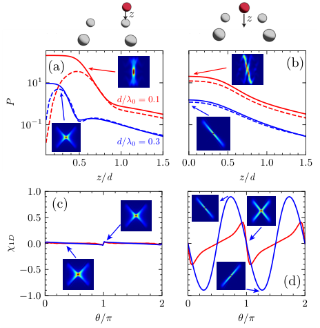
In Figs. 2(a) and 2(b), we plot the dependence of the Purcell factor on the vertical distance for emitters placed above an atom or at the center of the unit cell, respectively, as well as its emission pattern (insets). We compare both the semianalytical (solid lines) and the numerical approach (dashed lines) for two different distances, i.e., and in red and blue, respectively. Closer interatomic distances of the impurity atom to the metasurface lead to larger Purcell factors, although at the expense of losing the cross-directional emission, as expected from Figs. 1(d)-1(f). In addition, it is also at these small regions where we see the larger deviations between the semianalytical and numerical Purcell factors. These differences can be attributed to strong deviations from the Markovian behavior Sup, where is not expected to work, and can be attenuated by reducing , e.g., with a Raman transition. Apart from this deviation, another important difference of placing the impurity atom exactly above a metasurface atom [Fig. 2(a)] or at the center of the unit cell [Fig. 2(b)] is the tunability of the cross-directional emission shown in the inset of both panels. In particular, we can show that changing the relative orientation between the lattice and the impurity atom cancels the emission along one of the directions in the former case, but not in the latter. To characterize qualitatively this tunability, we define a directional parameter Sup,
| (8) |
where is the cumulative population of the dipoles located near a circle of radius centered on the emitter, and is its angle with respect to the axis. The maximum cumulative population is located at the angle . Cumulative population is renormalized so . With this definition, when the emission is purely one-dimensional, whereas when it becomes isotropic or emits in two orthogonal directions. In Figs. 2(c) and 2(d) we plot for the impurity positions of panels Figs. 2(a) and 2(b), respectively, showing that for certain with impurities at the center of the unit cell, whereas at all for the other case.

In Fig. 2, we see how, for the most tunable situation (), the Purcell factor is limited to . Now, we explore two possible strategies to boost while still preserving the possibility of tuning the directional emission patterns. The first strategy consists of placing pairs of emitters separated a distance and prepared in a given entangled state, e.g., . This can be done, e.g., using dynamical optical tweezers and local spin exchange Kaufman et al. 2015 or Rydberg interactions Wilk et al. 2010. The intuition is that the interference between the atomic emission within the cluster can lead to a cancellation of free-space emission and ultimately boost . This occurs for the antisymmetric case, obtaining , but at the price of losing the tunability of the directional emission (see Supplemental Material Sup). Since for this Letter, we are interested in keeping the tunability, in Fig. 3(c) we compare the numerically obtained for the symmetric cluster with the individual one for a dipole in the center of a plaquette at as a function of the cluster distance . Like this, one can get a moderate improvement for , but keeping the directional emission. Besides, we observe an effective rotation of the emission as increases, which shows that can be used as a tuning knob by itself. The other strategy consists of changing the metasurface structure by a bilayer one with separation , see scheme in Fig. 3(b). This structure also features straight isofrequencies Sup, where one can energetically tune the impurity atom to obtain directional emission patterns. In Fig. 3(d), we numerically obtain for the bilayer system and show how it can reach for either small distances, keeping the 1D tunability, or for but losing the 1D character of the emission.
After having characterized the single impurity coupling, let us consider how the directional emission patterns translate into collective dissipative interactions when more impurity atoms couple to the metasurface. One typical signature of these dissipative couplings is the lifetime renormalization of entangled atomic states Dicke 1954. This means that if an individual system decays with a rate , an entangled pair features a collective enhancement (decrease) of such decay rate depending on whether it is a super(sub) radiant configuration. In Fig. 4, we extract this collective enhancement as a function of the distance between impurities through a numerical fitting of the dynamics for the three different configurations explored in Figs. 2-3: namely, (i) for a pair of impurity atoms near the single-layer array (blue dots); (ii) for a pair of entangled atomic clusters near the single-layer array (green dots); and (iii) for a pair of impurity atoms within a shifted bilayer array (orange dots). In Fig. 4(a), we plot normalized to the impurity atom free-space individual decay rate . There we observe how, indeed, all strategies provide an improvement of collective effects compared to the case with no metasurface. To better compare the intrinsic collective dynamics induced in the different systems, in Fig. 4(b) we plot the same configurations, but normalizing to the individual decay rate in each configuration. There we observe how the bilayer enhances better collective effects at small distances due to its imperfect directionality, see Fig. 3(d), whereas the entangled cluster performs better at larger distances.
Summing up, we show how to obtain strongly directional emission patterns by placing atoms near quantum metasurfaces. We also study several strategies to achieve more efficient couplings between the impurity atoms and the directional subradiant modes of the metasurfaces based on entangled clusters or bilayer systems. Finally, we also show how these directional emission patterns translate into collective dissipative couplings when more impurity atoms couple to the metasurface. This shows the potential of quantum metasurfaces to induce nontrivial collective dissipative effects resulting from the interplay of interference and unconventional band structures. Our results can be of interest as well for subwavelength exciton arrays in 2D materials Reserbat-Plantey et al. 2021. An interesting outlook is to extend this analysis to the case topological band-structure models Perczel et al. 2017a; González-Tudela and Cirac 2018a; Perczel and Lukin 2020.
Acknowledgements.
A.G.-T. acknowledges financial support from the Proyecto Sinérgico CAM 2020 Y2020/TCS-6545 (NanoQuCo-CM), the CSIC Research Platform on Quantum Technologies PTI-001 and from Spanish project PGC2018-094792-B-100(MCIU/AEI/FEDER, EU). D.F.F acknowledges support from the CSIC JAE Intro Research program JAEINT-20-01823/EX-0330.Note added.-Recently, two works exploring similar ideas were published Castells-Graells et al. 2021; Zundel et al. 2022. The code to reproduce the figures of this Letter can be found in Fernandez-Fernandez 2022.
Supplemental Material: Tunable Directional Emission and Collective Dissipation with Quantum Metasurfaces
This Supplementary Material is divided as follows: in SM1 we explain in detail how to calculate the emergent band-structure of the single-layer metasurface, including the results for the in-plane and out-of-plane polarized modes; in Section SM2 we explain how to characterize impurity atom-metasurface coupling following both the semi-analytical approach of Ref. Asenjo-Garcia et al. 2017, and the numerical strategy that we design for this manuscript; in Section SM3 we provide more details on how to tune the directional emission; in Section SM4 we explain the improvement strategies developed in the main part of the manuscript based on entangled clusters and bilayer structures; in Section SM5 we explain the different configurations used to explore the collective superradiant dynamics of Fig. 4 of the main text; in Section SM6, we show that that similar phenomena can be found in other geometries by studying the emission pattern in a triangular geometry metasurface; finally, in Section SM7 we review the different experimental ingredients required to implement these ideas.
SM1 Band-structure of the single layer configuration
In this section, we are interested in characterizing completely the eigen-modes and eigen-energies of the sub-wavelength atomic array of Fig. 1(a) of the main manuscript. This quantum metasurface has a square geometry with primitive vectors , being the inter-atomic distance. The array has a total number of atoms, where denotes the linear size of the system. Thus, the position of the -th atom, can be described by two integer indices such that . For simplicity, we assume a two-level system description of the atoms. This means that the atoms only have a single optical transition between an excited and ground state denoted by and , respectively, with frequency and dipole polarization . In the main text, we only characterize the physics of the in-plane modes assuming . For completeness, here we will also calculate the emergent band-structure of the out-of-plane modes, , as well as the case of a circularly-polarized transition .
Irrespective of the polarization chosen, the dynamics of the subwavelength atomic array is described within a master equation formalism through the following Born-Markov master equation Lehmberg 1970a; Lehmberg 1970b:
| (SM1) |
where is an effective non-Hermitian Hamiltonian given by
| (SM2) |
where is a index running over the number of atoms of the metasurface, is the individual free-space decay rate, and the spin-dipole operator of the -th atom. The coherent () and incoherent () photon-mediated interactions among emitters are given by the vacuum’s Green Function Lehmberg 1970a; Lehmberg 1970b :
| (SM3) |
where:
| (SM4) |
with . Note these expressions of Eqs. (SM2)-(SM4) have already implicit the Born-Markov approximations Lehmberg 1970a; Lehmberg 1970b, which assumes that the frequency dependence of enters directly through the atomic frequency .
In the thermodynamic limit () the momentum is a good quantum number. This means that the Hamiltonian , in the single-excitation subspace, can be diagonalized using the Bloch functions as follows:
| (SM5) |
where takes values within the first Brillouin zone of the structure, that is . Each mode has then associated both a real () and imaginary () contribution to their energy given by
| (SM6) |
where is the discrete Fourier transform of the free-space tensor. Note that due to the long-range nature of the photon-mediated interactions of (see Eq.(SM4)), the sum in real space is slowly convergent. A method of avoiding that was proposed in Ref. Perczel et al. 2017b which consists in performing the summations in momentum space. This can be done using Poisson’s identity to write the sum in as a summation over reciprocal lattice vectors:
| (SM7) |
where is the area of the unit cell, and is the Weyl decomposition of the Green tensor, which is given by
| (SM8) |
Note that in Eq. (SM7) we separated the component because it provides a overall energy shift and it is mathematically divergent. Physically, this divergence is smeared out due to two effects: first, the system is finite and thus, one does not actually deal with infinite summation terms; second, the atoms are not point-dipole emitters, but rather have a well-defined finite size given by its ground-state atomic wavefunction size, . It can be shown that both terms by themselves renormalize the divergences and result in physical band-structures.
For example, in Ref. Perczel et al. 2017b, they obtained expressions for the renormalized Green tensor taking into account finite atomic size . This results into a convergent Green tensor at the origin:
| (SM9) |
where is the imaginary error function. On top of that, they also obtained the renormalization of the rest of the components of the Green tensor:
| (SM10a) | ||||
| (SM10b) | ||||
| (SM10c) | ||||
where we have defined the following expressions
| (SM11) |
| (SM12) |
| (SM13) |
| (SM14) |
An alternative approach consists in directly diagonalizing the Hamiltonian of Eq. (SM2) for a finite system. In that case, is not strictly a good quantum number, however, the eigenstates that are formally written as:
| (SM15) |
can be associated to a given -momentum of the Brillouin zone. To do it, one can perform the discrete Fourier transform of , i.e., , and see the that has the larger weight. In this section, and in Fig. 1 of the main text, we use this approach to estimate the that needs to be included for a given finite size, and then renormalize with a small to get is a more efficient way.
SM1.1 Results for in-plane polarized modes

In the main text we choose as the optimal inter-atomic distance to obtain the directional behaviour for the in-plane polarized modes. The justify this choice we include here in Fig. SM1 a systematic study of the metasurface band-structure for several distances. There, we first plot in Fig. SM1(a), to have it as a reference, the contour plot of the energy dispersion for the nearest-neighbour tight-binding model, i.e., , highlighting in dashed white the iso-frequency at the -mode energy responsible of the directional emission Galve et al. 2017; González-Tudela and Cirac 2017a; González-Tudela and Cirac 2017b. In SM1(b-d) we plot the emergent band-structure of the metasurface for several distances, where we observe how the straightness of the isofrequencies varies with the parameter . To characterize the straightness, we define a parameter that quantifies the difference of the isofrequencies with respect to the tight-binding model ones as follows:
| (SM16) |
where is the iso-frequency contour line obtained by solving . In Fig. SM1(e) we can see that there is a lattice constant that minimize the distance to the tight-binding iso-frequencies, which remarkably, is similar to the one where the highest value of the density of states is, see Fig. SM1(f).
SM1.2 Results for other polarizations: out-of-plane and circularly polarized transitions

For completeness, we also include here a similar study to the one performed in Fig. SM1, but for the out-of-plane modes. This is what we show in Fig. SM2(a-d), where we show the emergent band structure, , of a subwavelength atomic array with for several distances . As in the case in-plane polarized situation, displays saddle points at the X-point and a straightening of their corresponding isofrequencies. This is more evident when studying the difference of these isofrequencies with respect to the nearest-neighbour model defined by the parameter (see Eq. (SM16)), as shown in Fig. SM2(e). There, we observe how the optimal distance is (see Fig. SM2(g) for a line cut of ), also corresponds to a peak in the density of states, see Fig. SM2(f). At larger the model displays even a larger value of the density of states, however, this is also partly because other modes become resonant which will spoil directional emission, see Figs. SM2(b-d). Although this larger density of states leads to larger impurity coupling factors (as we will see in the next section), we decided to keep the discussion in the main text for the in-plane polarized modes since they have a less demanding optimal distance () and a more tunable directionality.

Finally, in Fig. SM3 we include the same analysis for the case where the optical transition is circularly polarized: . From the analysis of the band-structures and the -parameter, see Figs. SM3(a-f), the iso-frequencies become straighter, the smaller , i.e., there seems not to be an optimal one. However, for large , the superradiant modes become resonant with the subradiant -modes which can be detrimental for applications. In Fig. SM3(g), we finally provide an example of band-structure for showing how indeed it has a similar qualitative shape than the linearly-polarized modes.
SM2 Characterizing single impurity coupling to the metasurface
In this section, we will introduce an additional impurity atom together with the metasurface, as depicted in Fig. 1(a) of the main text. We denote as and to the frequency and polarization vector of its optical transition, such that its individual free-space decay rate reads . Thus, its intrinsic effective Hamiltonian can be written as . On top of that, this atom will exchange excitations with the metasurface through the same photon-mediated interactions appearing within the metasurface. The Hamiltonian describing such interaction is given by:
| (SM17) |
where :
| (SM18) |
Note that here there is already an implicit assumptions that to replace all the occurrences of by .
In what follows we are interested in characterizing the ratio of emission into the subradiant modes of the array () compared to the rest of the channels, e.g., free-space emission (). We denote this ratio as , which we label as the Purcell factor of the metasurface. In what follows we discuss two different methods to calculate it: a semi-analytical one in section SM2.1 and a full numerical approach in section SM2.2. These are the methods used to calculate the results of Figs. 2-3 of the main text. Here, for completeness, we will also use it to characterize the coupling of an impurity with an out-of-plane polarized array in section SM2.3.
SM2.1 Semi-analytical calculation of the impurity-metasurface coupling
Here, we extend the semi-analytical approach derived in Ref. Masson and Asenjo-Garcia 2020 for 1D subwavelength arrays to the metasurface situation. There, it was found that assuming a Born-Markov approximation for the impurity atom dynamics, the emission into the metasurface and free space modes can be calculated as follows:
| (SM19) | ||||
| (SM20) |
where is the position of the impurity atom, which is where we evaluate the eigen-modes defined as:
| (SM21a) | ||||
| (SM21b) | ||||
In Ref. Masson and Asenjo-Garcia 2020 an analytical expression was found for both and thanks to the 1D character of the modes. In our case, we can not find that expression, and we have to numerically calculate these integrals to obtain these values. We label as:
| (SM22) |
to the single impurity-metasurface Purcell factor calculated using this semi-analytical approach.
SM2.2 Numerical calculation of impurity-metasurface coupling
The other approach consists in initializing the impurity atom in the excited state, , and then compute the exact evolution of the system using the complete non-hermitian Hamiltonian of the combined impurity-metasurface system:
| (SM23) |
where . In this method we face two difficulties: i) how to avoid that the quantum emitter dynamics is affected by back-reflection of the subradiant excitations in finite systems; ii) how to extract the ratio from .
To tackle the first issue we impose non reflecting boundary conditions by including additional local losses in the dipoles close to the borders of the array. These additional losses must increase smoothly toward the ends of the lattices. For our calculations we find that a quadratic function is sufficient to avoid back scattering in most cases. The individual losses are given by:
| (SM24) |
with the distance from the center of the lattice at which the individual losses starts to increase, and the maximum distance from the outermost dipole in the array. We empirically find that the best results in our system are obtained with and .
In order to address the second issue, we use the fact that since conserves the number excitations, the wavefunction at any time can be written as:
| (SM25) |
from which we can monitor the total population in the impurity atom/lattice, i.e., and . The effective Hamiltonian induces a non-unitary dynamics, since the excitations can be eventually lost in free space. Thus, although , the sum for , where the difference with the initial population is the total loss into free-space of the system. This total loss can be also obtained by diagonalizing the quantum jump part of the master equation derived in Eq. SM1, i.e., , which leads to the following instantaneous quantum jump loss:
| (SM26) |
If the metasurface modes were perfectly subradiant, then the Purcell factor could be obtained just by dividing , since will give the decay of the impurity atom to free-space. In the simulation, however, we introduce absorbing boundaries, that we include in . These boundaries induce an additional decay of the metasurface modes to free-space that is artificially introduced by the simulation. Thus, it should be taken into account into the Purcell factor calculation to obtain a more accurate comparison with the semi-analytical procedure of Eqs. (SM19)-(SM20), which assumes an infinite size system. To estimate how much of the total losses, , are lost via the adiabatic absorbing boundaries, we assume that the hybridization of the absorber atoms with the rest of the metasurface is weak, such that, the losses in the border are given by
| (SM27) |
With that, we can add/substract these ”artificial” losses to each of the parts of the Purcell factor as follows:
| (SM28) |
When this value converges to a finite value, which is what we define as the numerical Purcell factor:
| (SM29) |
This procedure is the one we use in the main text to compare with the semi-analytical approach of Eq. (SM22). This method has several important advantages:
- •
It does not rely on Born-Markov approximation, and thus will be able to characterize impurity-metasurface couplings at all regimes.
- •
It can be easily generalized to calculate the Purcell factor of more general situations, such as the entangled cluster or bilayer configuration.
As we already observe for the in-plane polarized modes studied in the main text, both and display the same qualitative dependence with the system parameters, such as impurity-metasurface separation. The main quantitative difference appears in the regions where the Born-Markov approximation breaks, and the dynamics deviates significantly from a pure exponential decay. We explain this more in detail in the next section, where we characterize the impurity metasurface coupling for the out-of-plane transitions.
SM2.3 Results for out-of-plane emitters: non-Markovian dynamics

In Fig. SM4(a-b) we study the Purcell factor of an impurity atom with as a function of its vertical position for an array with out-of-plane polarized modes . In the two panels we plot the results for two different places of the unit cell depicted in the inset, as we did for the in-plane polarized modes in the main text. Compared to the case of the in-plane polarized modes, a noteworthy difference is that one can find regions with . This is expected since we already pointed that the narrower character of the band should lead to an increase of the density of states at the saddle-point divergence. Another important difference is that (dashed lines) and (markers) differ more than for the in-plane polarized metasurface. This points to the emergence of a more non-Markovian dynamics than in the in-plane polarized case. This is clear in Fig. SM4(c) (Fig. SM4(f)), we plot an example of the impurity atom dynamics in one of the points where the dynamics is (non-)Markovian, respectively. To make this more evident, in Figs. SM4(d-e) we plot a non-Markovianity witness of the dynamics introduced in Ref. Lorenzo et al. 2017 for the same parameters of Fig. SM4(a-b). This witness is defined as
| (SM30) |
in such a way that Markovian dynamics corresponds to , and for a perfect coherent oscillations, the hall-mark of non-Markovian dynamics. Comparing panels (a-b) with (d-e) we observe how indeed the regions of larger deviations feature a larger value of the non-Markovian witness. Although not shown, this out-of-plane polarization also leads to cross-like directional patterns, though less tunable than the in-plane polarized modes.
SM3 Directionality characterization
In order to characterize in more quantitative and qualitative terms the quasi-1D character of the emission patterns, we introduce a directional emission parameter, . To define it, we will calculate the amount of emission passed by the dipoles located at a given distance from the center of the lattice where we place our impurity atom. Since our array is discretized, we pick those dipoles based on a midpoint circle algorithm Agoston 2005. Then, we define the cumulative population of each of these selected dipoles as the integral over time
| (SM31) |
To compare the population of the dipoles in a concentric circle we redefine the cumulative population such that the sum over all dipoles in the circle is equal to one
| (SM32) |
Then we define the directionality as the sum of the populations for the dipoles located at a distance close to , weighted by a function which depends on the angle relative to the -axis
| (SM33) |
By working with the weight function , where is the angle of maximum population, we obtain that if the emission is a straight line. In Fig. 2(c-d) of the main manuscript we fixed always to for clarity of the figure, which is why we obtain negative values when the emission is orthogonal to it. Otherwise, if the emission is isotropic or cross-pattern like the nearest-neighbour hopping model, then . In order to mitigate the finite size effects, we compute for five concentric circles spaced at a distance of , and obtain the mean value of the directionality.
SM4 Improvement strategies: entangled-clusters and bilayers
In this section, we provide more details on the strategies we sketch in the main text to achieve larger Purcell factors in 2D subwavelength arrays.
SM4.1 Entangled clusters

The first strategy is to consider two impurity atoms separated at a subwavelength scale instead of a single one. We denote the distance from each impurity atom to the center of the cluster with , that will be subwavelength . The intuitive idea is that if we prepare this atomic cluster in an entangled state:
| (SM34) |
then the free-space emission between these two atoms can destructively interfere and boost the Purcell factor of the cluster, that we label as . In Fig. SM5(b-c) we calculate both and the associated directionality for the entangled cluster situation considered in the main text, and including both the symmetric (blue solid) and anti-symmetric configuration (dashed green) of the cluster. There, we observe how indeed the antisymmetric configuration can effectively achieved much larger ’s, but at expense of losing completely the tunability of the emission (though keeping the cross-directional emission pattern). We complement these figures with Fig SM5(a) that shows the individual Purcell factor for each of the impurity atoms within the cluster as they move from the center of the plaquette. There, we observe how the impurity atoms couple more efficiently to the metasurface around , which is where we observe an increase of for both the symmetric/antisymmetric configuration.
SM4.2 Bilayer configuration

The other strategy considered is to change the single layer metasurface by a bilayer one. We assume that the two layers are displaced from the plane at distances , while we will keep the auxiliary atoms at the plane. Here, we characterize numerically the band-structure of the bilayer in Fig. SM6(a-b) considering two situations: one where the bilayers are displaced between them (a), and another one where the layers are top of each other (b). In both cases, one can find subradiant mode regions that around the points, one obtains straight iso-frequencies Fig. SM6(c-d) leading to directional emission patterns, as shown in Fig. 3(c) of the main text.
SM5 Collective dynamics
In the main text, we explore the collective dynamics in three different initial configurations:
- •
The case of two separated single emitters at distance and initialized in a state:
(SM35) - •
The situation of two separated entangled clusters with intercluster separation , but separated between them at the same position :
(SM36) - •
The case of two separated atoms at distance among themselves and placed in-between a bilayer system with interlayer distance :
(SM37)
Using these initial states, we compute the dynamics using:
| (SM38) |
where the index denotes the different configurations. To estimate the strength of the collective effects we make a fit to an exponential decay law, i.e., , and plot , where is the value obtained by the individual decay at each configuration. In Fig. SM7, we plot a representative example of such dynamics and their corresponding emission patterns.

SM6 Other geometries
The existence of Van Hove singularities and straight iso-frequency lines is ubiquitous in two-dimensional geometries. Thus, the shaping of the radiation patterns and collective decays that we predict along this manuscript can be further observed and tuned with other types of metasurfaces. As an example, we plot in Figs. SM8 and Figs. SM9 the results obtained for a triangular geometry metasurface with interatomic spacing with perpendicular () and parallel () polarization vectors, respectively, see Fig. SM8(a) for a scheme. In Fig. SM8(c), we observe how the perpendicular polarized case indeed depicts straight iso-frequencies coinciding with the M-point, which is where the saddle point appear. The main difference with respect to the square metasurface is that the isofrequencies show an hexagonal shape instead of a square one. In Fig. SM8(b), we show how this point features a Van Hove singularity in the density of states, which leads to directional emission when an emitter is coupled resonantly to such energies, as depicted in Figs. SM8(d-e). The difference is that now that the emission occurs in six directions, instead of four, due to the different symmetry properties of the underlying geometry. In Fig. SM8(f-g), we further show how such emission can also be changed by changing the relative polarization between the impurity and the metasurface atoms, allowing to cancel partly the emission in some of the directions.

For completeness, we also show how the emission and interactions can be further tuned by changing the polarization of the metasurface atoms to be parallel to the metasurface plane, i.e., . This choice leads to a privileged direction and changes significantly the band-structure isofrequencies and density of states, see Fig. SM9(a-b). In particular, one does not have an hexagonal shape for the M-point isoequifrequencies. However, we find quite straight one-dimensional lines in the isofrequencies of the point, which enable quasi-1D and chiral emission depending on the relative orientation of the impurity atom polarization (see Figs. SM9(c-f)).

SM7 Experimental considerations
Although there are already good references in the literature where they explain how to implement the setup explored along this manuscript Masson and Asenjo-Garcia 2020; Patti et al. 2021; Brechtelsbauer and Malz 2021; Castells-Graells et al. 2021, for completeness we will just review here how to obtain the different experimental ingredients required for it:
- •
Subwavelength arrays. The key idea consists in using two different optical wavelengths for generating the optical lattice potentials that trap the atoms and for probing them. This was done, for example, in the recent experiment with Rb atoms Rui et al. 2020 where they use an isolated two-level transition of the D2 line for probing ( nm) and another one for generating the optical lattice nm, being able to achieve since the distance between the minima in the optical lattice is . To be able to reach the deeply subwavelength regime, Alkaline-Earth atoms, such as Ytterbium and Strontium, are more promising since they combine telecom with near ultra-violet transitions in their atomic energy spectrum Ludlow et al. 2015. For example, trapping Strontium at one its magic wavelengths Olmos et al. 2013 and driving through the telecom transition would enable Masson and Asenjo-Garcia 2020, whereas using the Ytterbium transitions (m) and ( nm) Covey et al. 2019, one could obtain .
- •
Impurity atoms control. For the trapping of the additional auxiliary atoms, one can initially trap them far from the metasurface with optical tweezers Kaufman et al. 2015, and then move the traps near it as in recent realizations with nanophotonic structures Dordevic et al. 2021. Regarding the control of its properties (frequency and linewidth), one can use a Raman-assisted transition with a -scheme Porras and Cirac 2008; Brechtelsbauer and Malz 2021; Castells-Graells et al. 2021, containing two hyperfine ground state levels, labelled as , connected to a common optically excited state (see Fig. SM10). The connection between the has to be done directly through a (detuned) classical laser field, or through a two-photon process, with overall amplitude and detuning . The transition has to be a cycling transition in such a way that the free-space photons only induce decay through that channel. Then, under the conditions , the dynamics of the optically excited state can be adiabatically eliminated, arriving to an effective two-level transition between the states which emits photons at frequencies , and with a renormalized linewidth . Thus, the dynamics can be made more or less Markovian by tuning the Raman factor . Relaxing the dynamical control requirement, another alternative is the use of other atomic isotopes which show similar atomic transitions but different linewidths Masson and Asenjo-Garcia 2020; Ludlow et al. 2015.
References
- Dicke (1954) R. H. Dicke, Phys. Rev. 93, 99 (1954).
- Gross and Haroche (1982) M. Gross and S. Haroche, Phys. Rep. 93, 301 (1982).
- Lehmberg (1970a) R. H. Lehmberg, Phys. Rev. A 2, 883 (1970a).
- Lehmberg (1970b) R. H. Lehmberg, Phys. Rev. A 2, 889 (1970b).
- Grimm et al. (2000) R. Grimm, M. Weidemüller, and Y. B. Ovchinnikov, in Advances In Atomic, Molecular, and Optical Physics (Elsevier, New York, 2000) pp. 95–170.
- Bloch et al. (2008) I. Bloch, J. Dalibard, and W. Zwerger, Rev. Mod. Phys. 80, 885 (2008).
- Deutsch et al. (1995) I. H. Deutsch, R. J. C. Spreeuw, S. L. Rolston, and W. D. Phillips, Phys. Rev. A 52, 1394 (1995).
- van Coevorden et al. (1996) D. V. van Coevorden, R. Sprik, A. Tip, and A. Lagendijk, Phys. Rev. Lett. 77, 2412 (1996).
- Klugkist et al. (2006) J. A. Klugkist, M. Mostovoy, and J. Knoester, Phys. Rev. Lett. 96, 163903 (2006).
- Antezza and Castin (2009a) M. Antezza and Y. Castin, Phys. Rev. Lett. 103, 123903 (2009a).
- Antezza and Castin (2009b) M. Antezza and Y. Castin, Phys. Rev. A 80, 013816 (2009b).
- Antezza and Castin (2013) M. Antezza and Y. Castin, Phys. Rev. A 88, 033844 (2013).
- Bartolo and Antezza (2014a) N. Bartolo and M. Antezza, Europhys. Lett. 107, 30006 (2014a).
- Bartolo and Antezza (2014b) N. Bartolo and M. Antezza, Phys. Rev. A 90, 033617 (2014b).
- Porras and Cirac (2008) D. Porras and J. I. Cirac, Phys. Rev. A 78, 053816 (2008).
- Scully (2015) M. O. Scully, Phys. Rev. Lett. 115, 243602 (2015).
- Asenjo-Garcia et al. (2017) A. Asenjo-Garcia, M. Moreno-Cardoner, A. Albrecht, H. J. Kimble, and D. E. Chang, Phys. Rev. X 7, 031024 (2017).
- Asenjo-Garcia et al. (2019) A. Asenjo-Garcia, H. J. Kimble, and D. E. Chang, Proc. Natl. Acad. Sci. U.S.A. 116, 25503 (2019).
- Zhang and Mølmer (2019) Y.-X. Zhang and K. Mølmer, Phys. Rev. Lett. 122, 203605 (2019).
- Bettles et al. (2016a) R. J. Bettles, S. A. Gardiner, and C. S. Adams, Phys. Rev. A 94, 043844 (2016a).
- Wang and Zhao (2018) B. X. Wang and C. Y. Zhao, Phys. Rev. A 98, 023808 (2018).
- Bettles et al. (2016b) R. J. Bettles, S. A. Gardiner, and C. S. Adams, Phys. Rev. Lett. 116, 103602 (2016b).
- Bettles et al. (2020) R. J. Bettles, M. D. Lee, S. A. Gardiner, and J. Ruostekoski, Commun. Phys. 3, 141 (2020).
- Shahmoon et al. (2017) E. Shahmoon, D. S. Wild, M. D. Lukin, and S. F. Yelin, Phys. Rev. Lett. 118, 113601 (2017).
- Perczel et al. (2017a) J. Perczel, J. Borregaard, D. E. Chang, H. Pichler, S. F. Yelin, P. Zoller, and M. D. Lukin, Phys. Rev. Lett. 119, 023603 (2017a).
- Perczel et al. (2017b) J. Perczel, J. Borregaard, D. E. Chang, H. Pichler, S. F. Yelin, P. Zoller, and M. D. Lukin, Phys. Rev. A 96, 063801 (2017b).
- Bettles et al. (2017) R. J. Bettles, J. Minář, C. S. Adams, I. Lesanovsky, and B. Olmos, Phys. Rev. A 96, 041603(R) (2017).
- Wild et al. (2018) D. S. Wild, E. Shahmoon, S. F. Yelin, and M. D. Lukin, Phys. Rev. Lett. 121, 123606 (2018).
- Glaetzle et al. (2017) A. W. Glaetzle, K. Ender, D. S. Wild, S. Choi, H. Pichler, M. D. Lukin, and P. Zoller, Phys. Rev. X 7, 031049 (2017).
- Grankin et al. (2018) A. Grankin, P. O. Guimond, D. V. Vasilyev, B. Vermersch, and P. Zoller, Phys. Rev. A 98, 043825 (2018).
- Guimond et al. (2019) P.-O. Guimond, A. Grankin, D. V. Vasilyev, B. Vermersch, and P. Zoller, Phys. Rev. Lett. 122, 093601 (2019).
- Poddubny (2020) A. N. Poddubny, Phys. Rev. A 101, 043845 (2020).
- Moreno-Cardoner et al. (2019) M. Moreno-Cardoner, D. Plankensteiner, L. Ostermann, D. E. Chang, and H. Ritsch, Phys. Rev. A 100, 023806 (2019).
- Bekenstein et al. (2020) R. Bekenstein, I. Pikovski, H. Pichler, E. Shahmoon, S. F. Yelin, and M. D. Lukin, Nat. Phys. 16, 676 (2020).
- Alaee et al. (2020) R. Alaee, B. Gurlek, M. Albooyeh, D. Martín-Cano, and V. Sandoghdar, Phys. Rev. Lett. 125, 063601 (2020).
- Masson and Asenjo-Garcia (2020) S. J. Masson and A. Asenjo-Garcia, Phys. Rev. Research 2, 043213 (2020).
- Patti et al. (2021) T. L. Patti, D. S. Wild, E. Shahmoon, M. D. Lukin, and S. F. Yelin, Phys. Rev. Lett. 126, 223602 (2021).
- Brechtelsbauer and Malz (2021) K. Brechtelsbauer and D. Malz, Phys. Rev. A 104, 013701 (2021).
- Wang et al. (2016) Z. Wang, F. Cheng, T. Winsor, and Y. Liu, Acs. Sym. Ser. 27, 412001 (2016).
- Glicenstein et al. (2020) A. Glicenstein, G. Ferioli, N. Šibalić, L. Brossard, I. Ferrier-Barbut, and A. Browaeys, Phys. Rev. Lett. 124, 253602 (2020).
- Rui et al. (2020) J. Rui, D. Wei, A. Rubio-Abadal, S. Hollerith, J. Zeiher, D. M. Stamper-Kurn, C. Gross, and I. Bloch, Nature 583, 369 (2020).
- Joannopoulos et al. (1997) J. D. Joannopoulos, P. R. Villeneuve, and S. Fan, Nature (London) 386, 143 (1997).
- Chang et al. (2018) D. E. Chang, J. S. Douglas, A. González-Tudela, C.-L. Hung, and H. J. Kimble, Rev. Mod. Phys. 90, 031002 (2018).
- Thompson et al. (2013) J. D. Thompson, T. G. Tiecke, N. P. de Leon, J. Feist, A. V. Akimov, M. Gullans, A. S. Zibrov, V. Vuletić, and M. D. Lukin, Science 340, 1202 (2013).
- Goban et al. (2014) A. Goban, C.-L. Hung, S.-P. Yu, J. Hood, J. Muniz, J. Lee, M. Martin, A. McClung, K. Choi, D. Chang, O. Painter, and H. Kimble, Nat. Commun. 5, 3808 (2014).
- Chang et al. (2019) T.-H. Chang, B. M. Fields, M. E. Kim, and C.-L. Hung, Optica 6, 1203 (2019).
- Burgers et al. (2018) A. P. Burgers, L. S. Peng, J. A. Muniz, A. C. McClung, M. J. Martin, and H. J. Kimble, Proc. Natl. Acad. Sci. U.S.A. 116, 456 (2018).
- Luan et al. (2020) X. Luan, J.-B. Béguin, A. P. Burgers, Z. Qin, S.-P. Yu, and H. J. Kimble, Adv. Quantum Technol. 3, 2000008 (2020).
- Béguin et al. (2020) J.-B. Béguin, J. Laurat, X. Luan, A. P. Burgers, Z. Qin, and H. J. Kimble, Proc. Natl. Acad. Sci. U.S.A. 117, 26109 (2020).
- Rusconi et al. (2021) C. C. Rusconi, T. Shi, and J. I. Cirac, Phys. Rev. A 104, 033718 (2021).
- Bello et al. (2019) M. Bello, G. Platero, J. I. Cirac, and A. González-Tudela, Sci. Adv. 5, eaaw0297 (2019).
- Leonforte et al. (2021) L. Leonforte, A. Carollo, and F. Ciccarello, Phys. Rev. Lett. 126, 063601 (2021).
- Bernardis et al. (2021) D. D. Bernardis, Z.-P. Cian, I. Carusotto, M. Hafezi, and P. Rabl, Phys. Rev. Lett. 126, 103603 (2021).
- García-Elcano et al. (2020) I. García-Elcano, A. González-Tudela, and J. Bravo-Abad, Phys. Rev. Lett. 125, 163602 (2020).
- García-Elcano et al. (2021) I. García-Elcano, J. Bravo-Abad, and A. González-Tudela, Phys. Rev. A 103, 033511 (2021).
- Bravo-Abad et al. (2012) J. Bravo-Abad, J. D. Joannopoulos, and M. Soljacic, Proc. Natl. Acad. Sci. U.S.A. 109, 9761 (2012).
- González-Tudela and Cirac (2018a) A. González-Tudela and J. I. Cirac, Phys. Rev. A 97, 043831 (2018a).
- Perczel and Lukin (2020) J. Perczel and M. D. Lukin, Phys. Rev. A 101, 033822 (2020).
- Galve et al. (2017) F. Galve, A. Mandarino, M. G. A. Paris, C. Benedetti, and R. Zambrini, Sci. Rep. 7, 42050 (2017).
- González-Tudela and Cirac (2017a) A. González-Tudela and J. I. Cirac, Phys. Rev. Lett. 119, 143602 (2017a).
- González-Tudela and Cirac (2017b) A. González-Tudela and J. I. Cirac, Phys. Rev. A 96, 043811 (2017b).
- Yu et al. (2019) S.-P. Yu, J. A. Muniz, C.-L. Hung, and H. J. Kimble, Proc. Natl. Acad. Sci. U.S.A. 116, 12743 (2019).
- González-Tudela and Cirac (2018b) A. González-Tudela and J. I. Cirac, Quantum 2, 97 (2018b).
- Hsu et al. (2016) C. W. Hsu, B. Zhen, A. D. Stone, J. D. Joannopoulos, and M. Soljačić, Nat. Rev. Mater. 1, 16048 (2016).
- Feiguin et al. (2020) A. Feiguin, J. J. García-Ripoll, and A. González-Tudela, Phys. Rev. Research 2, 023082 (2020).
- Paulisch et al. (2016) V. Paulisch, H. J. Kimble, and A. González-Tudela, New. J. Phys. 18, 043041 (2016).
- Kockum et al. (2018) A. F. Kockum, G. Johansson, and F. Nori, Phys. Rev. Lett. 120, 140404 (2018).
- (68) See Supplementary Material for more details on (i) how to calculate the band-structure and impurity-metasurface coupling, (ii) definition of the directionality parameter, (iii) improvement strategies, and (iv) collective dynamics of impurity atoms.
- Ludlow et al. (2015) A. D. Ludlow, M. M. Boyd, J. Ye, E. Peik, and P. O. Schmidt, Rev. Mod. Phys. 87, 637 (2015).
- Covey et al. (2019) J. P. Covey, I. S. Madjarov, A. Cooper, and M. Endres, Phys. Rev. Lett. 122, 173201 (2019).
- (71) Note, here we use the assumption commonly used in the literature that the free-space Green’s function does not vary significantly for the energy ranges around .
- Kaufman et al. (2015) A. M. Kaufman, B. J. Lester, M. Foss-Feig, M. L. Wall, A. M. Rey, and C. A. Regal, Nature (London) 527, 208 (2015).
- Wilk et al. (2010) T. Wilk, A. Gaëtan, C. Evellin, J. Wolters, Y. Miroshnychenko, P. Grangier, and A. Browaeys, Phys. Rev. Lett. 104, 010502 (2010).
- Reserbat-Plantey et al. (2021) A. Reserbat-Plantey, I. Epstein, I. Torre, A. T. Costa, P. A. D. Gonçalves, N. A. Mortensen, M. Polini, J. C. W. Song, N. M. R. Peres, and F. H. L. Koppens, ACS Photonics 8, 85 (2021).
- Castells-Graells et al. (2021) D. Castells-Graells, D. Malz, C. C. Rusconi, and J. I. Cirac, Phys. Rev. A 104, 063707 (2021).
- Zundel et al. (2022) L. Zundel, A. Cuartero-González, S. Sanders, A. I. Fernández-Domínguez, and A. Manjavacas, ACS Photonics 10.1021/acsphotonics.1c01463 (2022).
- Fernandez-Fernandez (2022) D. Fernandez-Fernandez, Davtax/Tunable-emission-metasurfaces: v1.0 (2022).
- Lorenzo et al. (2017) S. Lorenzo, F. Lombardo, F. Ciccarello, and G. M. Palma, Sci. Rep. 7, 42729 (2017).
- Agoston (2005) M. K. Agoston, Computer Graphics and Geometric Modeling (Springer-Verlag, Belin, 2005).
- Olmos et al. (2013) B. Olmos, D. Yu, Y. Singh, F. Schreck, K. Bongs, and I. Lesanovsky, Phys. Rev. Lett. 110, 143602 (2013).
- Dordevic et al. (2021) T. Dordevic, P. Samutpraphoot, P. L. Ocola, H. Bernien, B. Grinkemeyer, I. Dimitrova, V. Vuletić, and M. D. Lukin, Science 373, 1511 (2021).