On Variants of Facility Location Problem with Outliers
Abstract
In this work, we study the extension of two variants of the facility location problem (FL) to make them robust towards a few distantly located clients. First, -facility location problem (FL), a common generalization of FL and median problems, is a well studied problem in literature. In the second variant, lower bounded facility location (LBFL), we are given a bound on the minimum number of clients that an opened facility must serve. Lower bounds are required in many applications like profitability in commerce and load balancing in transportation problem. In both the cases, the cost of the solution may be increased grossly by a few distantly located clients, called the outliers. Thus, in this work, we extend FL and LBFL to make them robust towards the outliers. For FL with outliers (FLO) we present the first (constant) factor approximation violating the cardinality requirement by +1. As a by-product, we also obtain the first approximation for FLO based on LP-rounding. For LBFLO, we present a tri-criteria solution with a trade-off between the violations in lower bounds and the number of outliers. With a violation of in lower bounds, we get a violation of in outliers.
Keywords:
Facility Location Outliers Approximation Lower Bound -Facility Location -Median.1 Introduction
Consider an e-retail company that wants to open warehouses in a city for home delivery of essential items. Each store has an associated opening cost depending on the location in the city. The aim of the company is to open these warehouses at locations such that the cost of opening the warehouses plus the cost servicing all the customers in the city from the nearest opened store is minimised. In literature, such problems are called facility location problems(FL) where warehouses are the facilities and customers are the clients. Formally, in FL we are given a set of facilities and a set of clients. Each facility has an opening cost and cost of servicing a client from a facility is (we assume that the service costs are metric). The goal is to open a subset of facilities such that the cost of opening the facilities and servicing the clients from the opened facilities is minimised. In a variant of FL, called -facility location problem (FL), we are given an additional bound on the maximum number of warehouses/facilities that can be opened i.e. . In our example this requirement may be imposed to maintain the budget constraints or to comply with government regulations. In another variant of the problem, we are required to serve some minimum number of customers/clients from an opened facility. Such a requirement is natural to ensure profitability in our example. This minimum requirement is captured as lower bounds in facility location problems. That is, in lower bounded FL (LBFL), we are also given a lower bound on the minimum number of clients that an opened facility must serve.
In the above scenarios, a few distant customers/clients can increase the cost of the solution disproportionately; such clients are called outliers. Problem of outliers was first introduced by Charikar et al. [3] for the facility location and the -median problems. In this paper we extend -facility location and lower bounded facility location to deal with the outliers and denote them by FLO and LBFLO respectively. Since FL is well known to be NP-hard, NP-hardness of FLO and LBFLO follows. We present the first (constant factor) approximation for FLO opening at most facilities. In particular, we present the following result:
Theorem 1.1
There is a polynomial time algorithm that approximates -facility location problem with outliers opening at most facilities within times the cost of the optimal solution.
Our result is obtained using LP rounding techniques. As a by product, we get first constant factor approximation for FLO using LP rounding techniques. FLO is shown to have an unbounded integrality gap [3] with solution to the standard LP. We get around this difficulty by guessing the most expensive facility opened in the optimal solution. In particular we get the following:
Corollary 1
There is a polynomial time algorithm that approximates facility location problem with outliers within times the cost of the optimal solution.
We reduce LBFLO to FLO and use any algorithm to approximate FLO to obtain a tri-criteria solution for the problem. To the best of our knowledge, no result is known for LBFLO in literature. In particular, we present our result in Theorem 1.2 where a tri-criteria solution is defined as follows:
Definition 1
A tri-criteria solution for LBFLO is an - approximation solution that violates lower bounds by a factor of and outliers by a factor of with cost no more than where denotes the cost of an optimal solution of the problem, and .
Theorem 1.2
A polynomial time -approximation can be obtained for LBFLO problem where is a constant and is an approximation factor for the FLO problem.
Theorem 1.2 presents a trade-off between the violations in the lower bounds and that in the number of outliers. Violation in outliers can be made arbitrarily small by choosing close to . And, violation in lower bounds can be chosen close to at the cost of increased violation in the outliers. Similar result can be obtained for LBFLO with violation in cardinality using Theorem 1.1. The violation in the cardinality comes from that in FLO.
Our Techniques: For FLO, starting with an LP solution , we first eliminate the variables and work with an auxilliary linear programming (ALP) relaxation involving only variables. This is achieved by converting into a complete solution in which either or . Using the ALP, we identify the set of facilities to open in our solution. ALP is solved using iterative rounding technique to give a pseudo-integral solution (a solution is said to be pseudo integral if there are at most two fractional facilities). We open both the facilities at loss in cardinality and at a loss of factor in the cost by guessing the maximum opening cost of a facility in the optimal. Once we identify the set of facilities to open, we can greedily assign the first clients in the increasing order of distance from the nearest opened facility. Thus, in the rest of the paper, we only focus on identifying the set of facilities to open.
For LBFLO, we construct an instance of FLO by ignoring the lower bounds and defining new facility opening cost for each . An approximate solution to is obtained using any approximation algorithm for FLO. Facilities serving less than clients are closed and their clients are either reassigned to the other opened facilities or are made outliers. This leads to violation in outliers that is bounded by . Facility opening costs in are defined to capture the cost of reassignments.
Related Work: The problems of facility location and -median with outliers were first defined by Charikar et al. [3]. Both the problems were shown to have unbounded integrality gap [3] with their standard LPs. For FLO, they gave a -approximation using primal dual technique by guessing the most expensive facility opened by the optimal solution. For a special case of the problem with uniform facility opening costs and doubling metrics, Friggstad et al. [5] gave a PTAS using multiswap local search. For MO, Charikar et al. [3] gave a -approximation with -factor violation in outliers. Using local search techniques, Friggstad et al. [5] gave and -approximations with () violation in cardinality for general and doubling metric respectively. Chen [4] gave the first true constant factor approximation for the problem using a combination of local search and primal dual. Their approximation factor is large and it was improved to by Krishnaswamy et al. [10] by strengthening the LP. They use iterative rounding framework and, their factor is the current best result for the problem.
Lower bounds in FL were introduced by Karger and Minkoff [9] and Guha et al. [6]. They independently gave constant factor approximations with violation in lower bounds. The first true constant factor() approximation was given by Zoya Svitkina [12] for uniform lower bounds. The factor was improved to by Ahmadian and Swamy [1]. Shi Li [11] gave the first constant factor approximation for general lower bounds, with the constant being large (). Han et al. [7] studied the general lower bounded -facility location (LBFL) violating the lower bounds. Same authors [8] removed the violation in the lower bound for the -Median problem.
The only work that deals with lower bound and outliers together is by Ahmadian and Swamy [2]. They have given constant factor approximation for lower-bounded min-sum-of-radii with outliers and lower-bounded k-supplier with outliers problems using primal-dual technique.
2 solution for FLO
The problem FLO can be represented as the following integer program (IP):
| (1) | |||||
| (2) | |||||
| (3) | |||||
| (4) | |||||
| (5) |
where variable denotes whether facility is open or not and indicates if client is served by facility or not. Constraints 1 ensure that the extent to which a client is served is no more than . Constraints 2 ensure that a client is assigned only to an open facility. Constraint 3 ensures that the total number of facilities opened are atmost and Constraint 4 ensures that total number of clients served are at least . LP-Relaxation of the problem is obtained by allowing the variables . Let us call it .
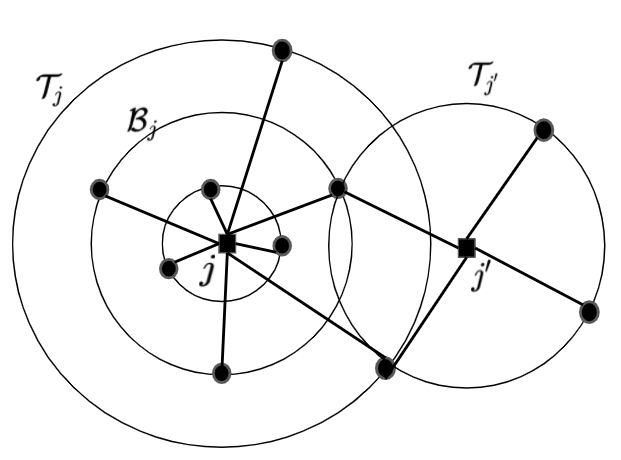
Let denote the optimal solution of and denote the cost of . A solution is said to be a complete solution either or , and . We first eliminate variables from our solution by making it complete. This is achieved by standard technique of splitting the openings and making collocated copies of facilities. For every client , we will define a bundle, as the set of facilities that are serving in our complete solution. Formally, . Let be the distance of farthest facility in from . See Fig. 1(). Note that the complete solution satisfies the following property:
- 1.
as .
- 2.
- 3.
as and .
2.1 Auxiliary LP (ALP)
 |
 |
| () | () |
.
We first discretize our distances , by rounding them to the nearest power of . Let , where is smallest power of such that . See Fig. 1(). Next, we identify a set of clients that are going to be served fully in our solution. Ideally, we would like to open at least one facility in for every . If all the ’s () were pair-wise disjoint, an LP constraint like for all , along with constraints 8(for partially served clients, say clients in ), 9(for cardinality) and 10(for outliers), is sufficient to get us a psuedo-integral solution. But this, in general, is not true. Thus we further identify a set so that we open one facility in for every and () ’s () are pair-wise disjoint (disjointness property) () for every , there is a close-by (within constant factor of distance from ) client in . On a close observation, we notice that instead of ’s, we are rather interested in smaller sets: let be the (rounded) distance of the farthest facility in serving in our solution and . Then we actually want ’s () to be pair-wise disjoint. As the distances are discretized, we have that is either or is . Since we don’t know , once a client is identified to be in , we search for it by starting with , and, shrinking it over iterations. Shrinking is done whenever, for , we obtain . Thus we add a constraint in our ALP and arrive at the following auxiliary LP (ALP). Variable denotes whether facility is opened in the solution or not. Constraints (9) and (10) correspond to the requirements of cardinality and outliers. For , if the ALP doesn’t open a facility within , it bounds the cost of sending up to a distance of .
| (6) | |||||
| (7) | |||||
| (8) | |||||
| (9) | |||||
| (10) | |||||
| (11) |
The following lemma gives a feasible solution to ALP such that cost is bounded by LP optimal within a constant factor.
Lemma 1
A feasible solution can be obtained to the ALP such that .
Proof
∎
2.2 Iterative Rounding
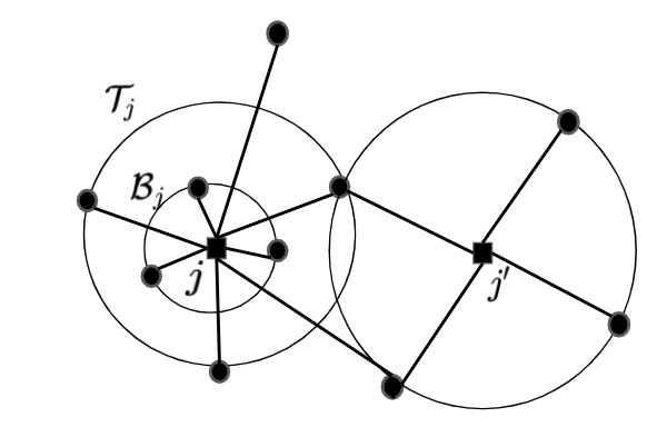
We next present an iterative rounding algorithm(IRA) for solving the ALP. In every iteration of IRA, we compute an extreme point solution to ALP and check whether any of the constraints 7 or 8 has become tight. If a constraint corresponding to gets tight, we move the client to and remove it from . We also update so that disjointness property is satisfied. If a constraint corresponding to gets tight, we shrink to ; update and accordingly. The algorithm is formally stated in Algorithm 1. For , let be the client who takes the responsibility of getting served. Whenever is added to is set to and whenever it is removed because of another client , is set to . If was never added to , then there must be a because of which it was not added to in lines and . Such a takes the responsibility of in that case. Note that a client may be added and removed several times from over the iterations of the algorithm as and shrink (see Fig. 2 for illustration).
 |
 |
 |
| () | () | () |
Lemmas 2, 3, and 4 help us analyse our algorithm. Lemma 2 shows that the solution obtained in an iteration is feasible for the ALP of the next iteration. We also prove that the cost of the solutions computed is non-increasing over iterations.
Lemma 2
Let and be the auxiliary LPs before and after iteration of IRA. Let be the extreme point solution obtained in iteration. Then is a feasible solution to , and hence .
Proof
Note that the feasibility and the cost can change only when one of constraints (7) or constraints (8) becomes tight, that is, either condition at step 4 or condition at step 6 of the algorithm is true.
- ()
When one of constraints (8) corresponding to a client becomes tight i.e. , we move client from to and define the set . Thus, . Thus the new constraints added in constraints 7 and 6 (if is added to ) are satisfied. Constraint (10) holds as increases by and decreases by . There is no change in constraint 9.
Let one of the constraints (7) corresponding to a full client becomes tight i.e. . Two things happen here: () we shrink to , hence . Thus constraint 6 is satisfied if is added to . () shrink to half its radius, thus . Thus constraint 7 corresponding to continue to be satisfied with the shrunk . There is no change in constraints 9 and 10.
- ()
For a client , let , and be the set , and corresponding to client in and , and be the respective values in .
- a.
When and shrink because constraint 7 becomes tight for a client . Cost paid by in in the iteration because in the iteration. Since , Cost paid by in in the iteration. Thus change in cost is .
- b.
When a client is moved from to because constraint 8 becomes tight. Cost paid by in in the iteration Cost paid by in in the iteration. Thus change in cost is .
- a.
∎
Thus we have, where the first inequality follows because is an extreme point solution and is a feasible solution to . Hence, if is the number of iterations of the IRA then where the second last inequality follows as is an extreme point solution and is a feasible solution for , last inequality follows from Lemma 1. Let be the solution returned by the IRA, then . Lemma 3 establishes that at the end of our IRA, solution is pseudo-integral.
Lemma 3
returned by Algorithm 1 has at most two fractionally opened facilities.
Proof
At the termination of the algorithm constraints 7 and 8 will not be tight. Let be the number of fractional variables at the end of the algorithm. Then there are exactly number of independent tight constraints from (6), (9) and (10). Let be the number of tight constraints of type 6. There must be at least fractional variables corresponding to each of these constraints. Also, there must be at least fractional variables corresponding to constraint 6, different from those obtained constraints 10. Thus, i.e. . Also, the number of tight constraints is at most and hence is at most giving us or .
∎
We open both the fractionally opened facilities at a loss of in the facility opening cost where is the guess of the most expensive facility opened by the optimal. In Lemma 4 we show that for a client in there is some client in , that is close to , i.e. within distance of .
Lemma 4
At the conclusion of the algorithm, for every , there exists at least 1 unit of open facilities within distance from j. Formally, .
Proof
Let . If , then this means that was added to and was present in at the end of the algorithm. Then, one unit is open in i.e. within a distance of of .
If then was either never added to or was removed later. In either case responsibility of opening a facility in a close vicinity of was taken by . First we consider the case when was added to but removed later. Let be the sequence of clients such that and . Since , one unit is open in i.e. within a distance of of . Clearly, . Thus for all . Thus, . Thus one unit of facility is open within a distance of from .
Next, let was never added to . Then since , was added to at some point of time. Thus, from above one unit of facility is opened within distance of . Also, . Thus, one unit of facility is opened within distance of .
∎
We run the algorithm for all the guesses of and select the one with the minimum cost.
Combining Everything: Let be our final solution. where is the cost of the optimal solution.
3 Tri-criteria for LBFLO
In this section, we present a tri-criteria solution for LBFLO problem with -factor violation in lower bound and at most -factor violation in outliers at ()-factor loss in cost where is approximation for FLO. Let be an instance of LBFLO. For a facility , let be the set of nearest clients. We construct an instance of FLO with lower bounds ignored and facility costs updated as follows: if a facility is opened in optimal solution of , then it pays at least cost for serving clients. Therefore, where is a tunable parameter.
Lemma 5
Optimal solution of is bounded by where is the optimal solution of .
Proof
Clearly is a feasible solution for . Thus, service cost is same as that in . And, . Therefore, .
∎
Once we have an instance of FLO, we use any algorithm for FLO to get a solution to of cost no more than where is the optimal solution of and is approximation solution for FLO. Note that a facility opened in solution might serve less than clients as we ignored the lower bounds in instance . We close such facilities and do some reassignments to improve the violation in the lower bounds to ; in the process we make some violation in the number of outliers.
We convert the solution to a solution of LBFLO. We close every facility that is serving less than clients in and either reassign its clients to other opened facilities or decide to leave them unserved. Cost of reassignment is charged to the facility opening costs of the closed facilities. Consider a facility opened in that served less than clients. Let be the set of clients, in , assigned to in and be the remaining clients in . Since serves clients, . Some of the clients in are outliers in and some are assigned to other facilities. Let be the clients in that are outliers and be the clients in assigned to some other facilities. See Fig. 3(). If then let be the nearest client to . then,
| (12) |
 |
 |
| () | () |
Clients in are assigned to the facilities serving the clients in and are made outliers proportionally. That is, we assign clients in to the nearest facility opened in and leave clients in unserved. If , then the total cost of reassignment is (as was assigned to and not to in ) (using (12)) (As and ) (for ). Thus the additional cost of reassignment of clients in is bounded by the facility opening cost of . Violation in outliers is .
Overall Cost Bound: It is easy to see that as cost of solution is sum of the original connection cost which is equal to the connection cost of , () the additional cost of reassignment, which is paid in by facilities that are closed in and, () the facility cost of the remaining facilities. Thus, for . Using -approximation of Charikar et al. [3] for FLO, we get factor loss in cost for .
4 Conclusion and Future Scope
In this paper, we first presented a -factor approximation for -facility location problem with outliers opening at most facilities. This also gives us the first constant factor approximation for FLO using LP rounding techniques. Our result can be extended to knapsack median problem with outliers with violation in budget using enumeration techniques.
We also gave a tri-crtieria, -solution for general LBFLO where and . It will be interesting and challenging to see if we can reduce the violation in outliers to maintaining .
We believe that using pre-processing and strengthened LP techniques of Krishnaswamy et al. [10] we can get rid of the violation in cardinality for FLO. This will also directly extend our tri-criteria solution to lower bounded -facility location problem with outliers (LBFLO).
References
- [1] Ahmadian, S., Swamy, C.: Improved approximation guarantees for lower-bounded facility location. In: Erlebach, T., Persiano, G. (eds.) Approximation and Online Algorithms. pp. 257–271. Springer Berlin Heidelberg, Berlin, Heidelberg (2013)
- [2] Ahmadian, S., Swamy, C.: Approximation Algorithms for Clustering Problems with Lower Bounds and Outliers. In: Chatzigiannakis, I., Mitzenmacher, M., Rabani, Y., Sangiorgi, D. (eds.) 43rd International Colloquium on Automata, Languages, and Programming (ICALP 2016). Leibniz International Proceedings in Informatics (LIPIcs), vol. 55, pp. 69:1–69:15. Schloss Dagstuhl–Leibniz-Zentrum fuer Informatik, Dagstuhl, Germany (2016). https://doi.org/10.4230/LIPIcs.ICALP.2016.69, http://drops.dagstuhl.de/opus/volltexte/2016/6215
- [3] Charikar, M., Khuller, S., Mount, D.M., Narasimhan, G.: Algorithms for facility location problems with outliers. In: Proceedings of the Twelfth Annual ACM-SIAM Symposium on Discrete Algorithms. p. 642–651. SODA ’01, Society for Industrial and Applied Mathematics, USA (2001)
- [4] Chen, K.: A constant factor approximation algorithm for k-median clustering with outliers. In: Proceedings of the Nineteenth Annual ACM-SIAM Symposium on Discrete Algorithms. p. 826–835. SODA ’08, Society for Industrial and Applied Mathematics, USA (2008)
- [5] Friggstad, Z., Khodamoradi, K., Rezapour, M., Salavatipour, M.R.: Approximation schemes for clustering with outliers. ACM Trans. Algorithms 15(2), 26:1–26:26 (2019). https://doi.org/10.1145/3301446, https://doi.org/10.1145/3301446
- [6] Guha, S., Meyerson, A., Munagala, K.: Hierarchical placement and network design problems. In: Proceedings of the 41st Annual Symposium on Foundations of Computer Science. p. 603. FOCS ’00, IEEE Computer Society, USA (2000)
- [7] Han, L., Hao, C., Wu, C., Zhang, Z.: Approximation algorithms for the lower-bounded k-median and its generalizations. In: Kim, D., Uma, R.N., Cai, Z., Lee, D.H. (eds.) Computing and Combinatorics. pp. 627–639. Springer International Publishing, Cham (2020)
- [8] Han, L., Hao, C., Wu, C., Zhang, Z.: Approximation algorithms for the lower-bounded knapsack median problem. In: Zhang, Z., Li, W., Du, D.Z. (eds.) Algorithmic Aspects in Information and Management. pp. 119–130. Springer International Publishing, Cham (2020)
- [9] Karget, D.R., Minkoff, M.: Building steiner trees with incomplete global knowledge. In: Proceedings 41st Annual Symposium on Foundations of Computer Science. pp. 613–623 (2000). https://doi.org/10.1109/SFCS.2000.892329
- [10] Krishnaswamy, R., Li, S., Sandeep, S.: Constant approximation for k-median and k-means with outliers via iterative rounding. In: Proceedings of the 50th Annual ACM SIGACT Symposium on Theory of Computing. p. 646–659. STOC 2018, Association for Computing Machinery, New York, NY, USA (2018). https://doi.org/10.1145/3188745.3188882, https://doi.org/10.1145/3188745.3188882
- [11] Li, S.: On facility location with general lower bounds. In: Proceedings of the Thirtieth Annual ACM-SIAM Symposium on Discrete Algorithms. p. 2279–2290. SODA ’19, Society for Industrial and Applied Mathematics, USA (2019)
- [12] Svitkina, Z.: Lower-bounded facility location. ACM Trans. Algorithms 6(4) (Sep 2010). https://doi.org/10.1145/1824777.1824789, https://doi.org/10.1145/1824777.1824789