Electron-magnon coupling and quasiparticle lifetimes on the surface of a topological insulator

The Hamiltonian describing the interface between the TI and the FM contains a lattice formulation of the TI surface, $H_{\textrm{TI}}$, a Heisenberg model for the FM with an additional easy-axis anisotropy term, $H_{\textrm{FM}}$, and a model for the exchange coupling of lattice site spins in the FM to the electrons on the TI surface, $H_{\textrm{int}}$. We use the same model presented in Ref. Erlandsen et al. 2020, namely, $H=H_{\textrm{TI}}+H_{\textrm{FM}}+H_{\textrm{int}}$, with

Here, $v_{\textrm{F}}$ is the Fermi velocity, $\boldsymbol{c}_{i}^{\dagger}=(c_{i\uparrow}^{\dagger},c_{i\downarrow}^{\dagger})$, the fermionic operators $c_{i\sigma}^{\dagger}$ and $c_{i\sigma}$ create and destroy electrons with spin $\sigma$ at lattice site $i$, respectively, $\boldsymbol{\tau}=(\tau_{x},\tau_{y},\tau_{z})$ are the Pauli matrices, and H.c. denotes the Hermitian conjugate of the preceding term. Furthermore, $\hat{x}$ and $\hat{y}$ are unit vectors in the $x$ direction and $y$ direction, respectively, $\mu$ is the chemical potential, and $\langle i,j\rangle$ indicates that the lattice sites $i$ and $j$ located at $\boldsymbol{r}_{i}$ and $\boldsymbol{r}_{j}$ should be nearest neighbors. To ease computational requirements, we have assumed a 2D square lattice in the interfacial plane. The first line of $H_{\textrm{TI}}$ represents the spin-momentum locking of electrons on the TI surface. The Wilson terms containing $W$ are added to avoid additional Dirac cones at the Brillouin zone boundaries appearing from a direct discretization of the continuum model Zhou et al. 2017. They are added so that the lattice model reproduces the correct physics Erlandsen et al. 2020; Zhou et al. 2017. The FM Hamiltonian contains an exchange interaction between nearest-neighbor lattice site spins, $\boldsymbol{S}_{i}$, with strength $J>0$, and an easy-axis anisotropy term determined by $K>0$ ensuring that ordering in the $z$ direction is energetically favorable. The interfacial exchange coupling is parametrized by $\bar{J}$.

The next step is to obtain the fermions which diagonalize the TI Hamiltonian and the magnons which diagonalize the FM Hamiltonian. This was performed in Ref. Erlandsen et al. 2020 and we repeat the main points here. A Holstein-Primakoff (HP) transformation Holstein and Primakoff 1940 is introduced for the spin operators $S_{i+}=\sqrt{2S}a_{i}$, $S_{i-}=\sqrt{2S}a_{i}^{\dagger}$, and $S_{iz}=S-a_{i}^{\dagger}a_{i}$, where the bosonic operators $a_{i}^{\dagger}$ and $a_{i}$ create and destroy magnons at lattice site $i$, respectively. Furthermore, $S_{i\pm}=S_{ix}\pm iS_{iy}$, while $S$ is the spin quantum number of the lattice site spins. Here, we have neglected any terms beyond quadratic in the magnon operators $a_{i}$, and we continue to do so throughout the analysis. This is permissible when assuming that the spins are nearly ordered, with only small quantum fluctuations, even when $S$ is not large. Additionally, any constant terms in the Hamiltonian are neglected as these merely shift the zero point of the energy. Performing a Fourier transform (FT) on the magnon operators, $a_{i}=\frac{1}{\sqrt{N}}\sum_{\boldsymbol{q}}a_{\boldsymbol{q}}e^{-i\boldsymbol{q}\cdot\boldsymbol{r}_{i}}$, where $N$ is the number of lattice sites on the interface, gives

with $\omega_{\boldsymbol{q}}=2KS+4JS(2-\cos q_{x}-\cos q_{y})$. Notice the gap in the magnon spectrum due to the easy-axis anisotropy, $2KS$. The easy-axis anisotropy stabilizes the ground state with magnetization in the $z$ direction, and a higher energy is needed to excite spin fluctuations. We refer to $\boldsymbol{q}$ as the momentum of the magnon, even though, since we have set $\hbar=a=1$, it is technically a dimensionless version of the quasimomentum, restricted to the first Brillouin zone (1BZ) of the 2D square lattice.

Inserting the HP transformation, as well as a FT of both the magnon and the electron operators, $c_{i\sigma}=\frac{1}{\sqrt{N}}\sum_{\boldsymbol{k}}c_{\boldsymbol{k}\sigma}e^{-i\boldsymbol{k}\cdot\boldsymbol{r}_{i}}$, into $H_{\textrm{int}}$ yields

Here, $V=-2\bar{J}\sqrt{2S}$, $\sigma=1$ for spin up, and $\sigma=-1$ for spin down. The first line describes EMC involving one magnon, while terms showing EMC with more than one magnon have been neglected. We have also neglected any Umklapp processes, since a small Fermi surface close to the 1BZ center means the Fermi momentum is much smaller than the reciprocal lattice vectors Erlandsen et al. 2020. The terms in the second line do not contain magnon operators and are therefore moved to $H_{\textrm{TI}}$. These terms act like an external magnetic field on the TI and will open a gap in the fermionic spectrum. This is due to the magnetization along the $z$ direction in the FM.

Next, the electron operators in $H_{\textrm{TI}}$ are FT and a unitary transformation is used to diagonalize the Hamiltonian in terms of quasiparticles $\psi_{\boldsymbol{k}\eta}$ with the helicity band index $\eta=\pm$,

The excitation energies are $E_{\boldsymbol{k}\eta}=-\mu+\eta F_{\boldsymbol{k}}$, where we define $B_{\boldsymbol{k}}=W(2-\cos k_{x}-\cos k_{y})-2\bar{J}S$, $C_{\boldsymbol{k}}=-v_{\textrm{F}}\sin k_{y}$, $D_{\boldsymbol{k}}=-v_{\textrm{F}}\sin k_{x}$, and $F_{\boldsymbol{k}}=\sqrt{B_{\boldsymbol{k}}^{2}+C_{\boldsymbol{k}}^{2}+D_{\boldsymbol{k}}^{2}}$. Also defining $N_{\boldsymbol{k}}=2F_{\boldsymbol{k}}(F_{\boldsymbol{k}}+B_{\boldsymbol{k}})$, the electron operators are related to the quasiparticle operators as

with transformation coefficients

The TI excitation spectrum is plotted in Fig. 2. The exchange coupling has introduced a gap of $4\bar{J}S$ in the original Dirac cone, similar to a mass gap for massive Dirac fermions Wehling et al. 2014. The Wilson terms open gaps at the boundaries of the 1BZ, ensuring that there is only one Dirac cone present in the system Zhou et al. 2017.

Finally transforming $H_{\textrm{int}}$ to the basis which diagonalizes $H_{\textrm{TI}}$ gives

At this point our calculations diverge from those of Ref. Erlandsen et al. 2020, as we now calculate the self-energy of the fermionic quasiparticles due to EMC. We include nonzero temperature by going to a sum over Matsubara frequencies and find Bruus and Flensberg 2004; Abrikosov et al. 1963; Mahan 2000; Giraud and Egger 2011; Calandra and Mauri 2007; Park et al. 2007; Tse and Das Sarma 2007

based on the sunset Feynman diagrams presented in Fig. 3. Hence, we have truncated our calculation of the self-energy at second order in the EMC, employing the Migdal approximation Migdal 1958; Park et al. 2007. We have also used the fact that the tadpole diagram gives zero contribution in the systems considered in this paper, as shown in Appendix A. $\chi$ labels the direction of the magnon, i.e., the sign in front of $\boldsymbol{q}$, while $\lambda$ labels the magnon mode, which for the FM case is superfluous. Based on Eq. (II.1) we have, e.g., the coupling constant $g_{\boldsymbol{k}+\boldsymbol{q},\boldsymbol{k},\chi=+}^{\eta\eta^{\prime}}=VQ_{\downarrow\eta}^{*}(\boldsymbol{k}+\boldsymbol{q})Q_{\uparrow\eta^{\prime}}(\boldsymbol{k})$.

The bare fermion Green’s function is Abrikosov et al. 1963; Bruus and Flensberg 2004 $G_{0}^{\eta}(\boldsymbol{k},i\omega_{n})=1/(i\omega_{n}-E_{\boldsymbol{k}\eta})$, with $\omega_{n}=(2n+1)\pi T$. Upon introducing $\omega_{\nu}=2\pi\nu T$, we use the bare magnon Green’s function Bruus and Flensberg 2004 $D_{0}^{\chi}(\boldsymbol{q},i\omega_{\nu})=\chi/(i\omega_{\nu}-\chi\omega_{\boldsymbol{q}})$ for the magnon operator $a_{\boldsymbol{q}}$ when $\chi=+$ and $a_{-\boldsymbol{q}}^{\dagger}$ when $\chi=-$, both with dispersion $\omega_{\boldsymbol{q}}$. Hence, we use separate propagators for $a_{\boldsymbol{q}}$ and $a_{-\boldsymbol{q}}^{\dagger}$ as opposed to, e.g., EPC where one usually finds the propagator of the sum of these Tse and Das Sarma 2007. In other words, the magnons moving forward and backward in time are treated separately, before adding their respective contributions.

We first perform the sum over the Matsubara frequencies Bruus and Flensberg 2004; Mahan 2000,

Here, $B_{\text{E}}(\epsilon)=1/(e^{\epsilon/T}-1)=[\coth(\epsilon/2T)-1]/2$ is the Bose-Einstein distribution and $F_{\text{D}}(\epsilon)=1/(e^{\epsilon/T}+1)=[1-\tanh(\epsilon/2T)]/2$ is the Fermi-Dirac distribution. Using $B_{\text{E}}(-\epsilon)=-1-B_{\text{E}}(\epsilon)$ and an analytic continuation $i\omega_{n}\to\omega+i\delta$, where $\delta=0^{+}$ Mahan 2000; Park et al. 2007; Tse and Das Sarma 2007, yields

The following transformation is used in the sum over momentum:

Inserting Eqs. (II.2) and (15) into Eq. (II.2) gives

We use the same model presented in Ref. Erlandsen et al. 2020, namely, $H=H_{\textrm{TI}}+H_{\textrm{AFM}}+H_{\textrm{int}}$, with

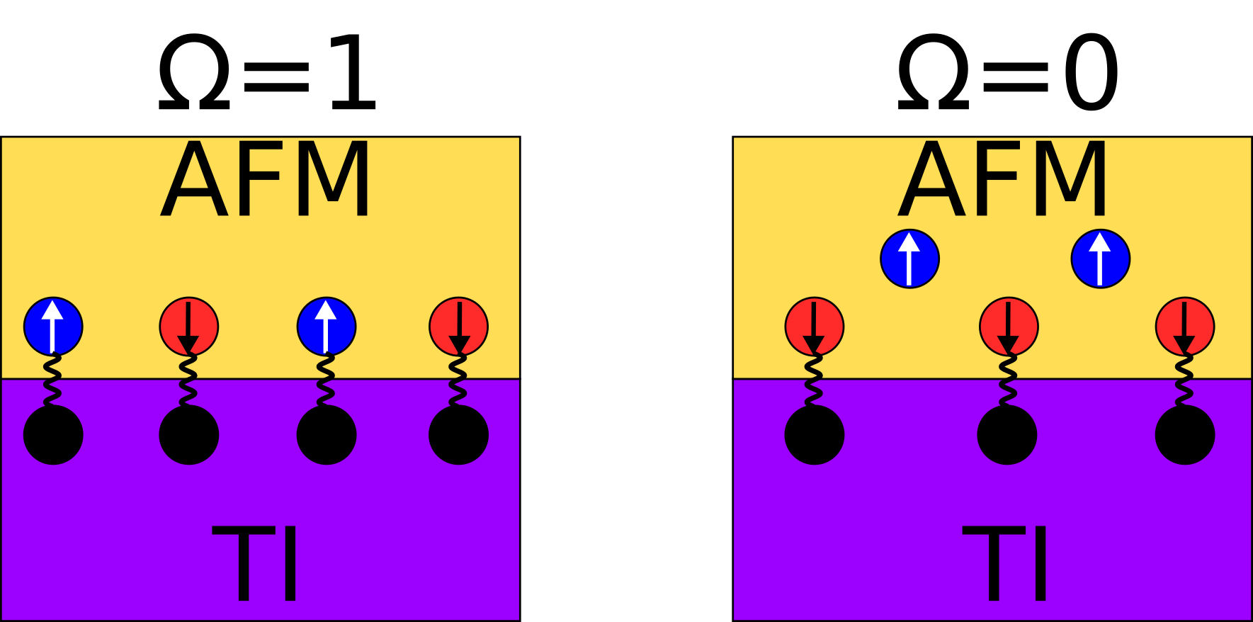
and $H_{\textrm{TI}}$ as in Eq. (1). Here, $\langle\langle i,j\rangle\rangle$ indicates that the lattice sites $i$ and $j$ should be next-nearest neighbors. Once again, we have assumed a 2D square lattice in the interfacial plane for computational convenience. The AFM Hamiltonian contains an exchange interaction between nearest-neighbor lattice site spins with strength $J_{1}>0$ and between next-nearest neighbors with strength $J_{2}$. If $J_{2}<0$ this term stabilizes the AFM state, while if $J_{2}>0$ it acts as a frustration. We assume $|J_{2}|\ll J_{1}$ such that the system remains in the staggered state also for $J_{2}>0$. The easy-axis anisotropy term is the same as in the FM case. The sublattices of the bipartite lattice in the AFM are labeled $A$ and $B$. The exchange coupling to the electrons on the TI surface is parametrized by $\bar{J}_{A}$ and $\bar{J}_{B}$ for lattice site spins on the $A$ and $B$ sublattices, respectively. We allow $\bar{J}_{A}$ and $\bar{J}_{B}$ to be different, which can describe an uncompensated antiferromagnetic interface where one sublattice is more exposed than the other Erlandsen et al. 2020. This is illustrated in Fig. 4. We introduce $\bar{J}\equiv\bar{J}_{B}$ and $\Omega\equiv\bar{J}_{A}/\bar{J}_{B}$, and let $0\leq\Omega\leq 1$ parametrize the sublattice asymmetry of the exchange coupling.

Obtaining the eigenexcitations of the TI and the AFM follows a similar methodology as the FM case Erlandsen et al. 2020, and we focus on the main differences. We assume the lattice site spins on the $A$ sublattice point in the positive $z$ direction and opposite alignment on the $B$ sublattice. A HP transformation is introduced for the spin operators $S_{i+}^{A}=\sqrt{2S}a_{i}$, $S_{i-}^{A}=\sqrt{2S}a_{i}^{\dagger}$, $S_{iz}^{A}=S-a_{i}^{\dagger}a_{i}$, $S_{i+}^{B}=\sqrt{2S}b_{i}^{\dagger}$, $S_{i-}^{B}=\sqrt{2S}b_{i}$, and $S_{iz}^{B}=-S+b_{i}^{\dagger}b_{i}$. Next, we introduce FT of the magnon operators, $a_{i}=\frac{1}{\sqrt{N_{A}}}\sum_{\boldsymbol{q}\in\Diamond}a_{\boldsymbol{q}}e^{-i\boldsymbol{q}\cdot\boldsymbol{r}_{i}}$ and $b_{i}=\frac{1}{\sqrt{N_{B}}}\sum_{\boldsymbol{q}\in\Diamond}b_{\boldsymbol{q}}e^{-i\boldsymbol{q}\cdot\boldsymbol{r}_{i}}$. Here, $N_{A}$ and $N_{B}$ are the number of lattice sites in the sublattices, and we assume $N_{A}=N_{B}=N/2$, where $N$ is the total number of lattice sites on the interface. The sums over $\boldsymbol{q}$ are restricted to the reduced Brillouin zone (RBZ) of the sublattices, which is indicated by $\boldsymbol{q}\in\Diamond$. $H_{\textrm{AFM}}$ is not diagonal in the original sublattice magnons $a_{\boldsymbol{q}}$ and $b_{\boldsymbol{q}}$. Hence, a Bogoliubov transformation is introduced, expressing new magnon operators as $\alpha_{\boldsymbol{q}+}=u_{\boldsymbol{q}}a_{\boldsymbol{q}}-v_{\boldsymbol{q}}b_{-\boldsymbol{q}}^{\dagger}$ and $\alpha_{\boldsymbol{q}-}=u_{\boldsymbol{q}}b_{\boldsymbol{q}}-v_{\boldsymbol{q}}a_{-\boldsymbol{q}}^{\dagger}$. Requiring that the new operators are bosonic fixes $|u_{\boldsymbol{q}}|^{2}-|v_{\boldsymbol{q}}|^{2}=1$. We assume $u_{\boldsymbol{q}}$ and $v_{\boldsymbol{q}}$ are real, as well as inversion symmetric in $\boldsymbol{q}$. Requiring that the AFM Hamiltonian is diagonal in terms of these new magnon operators yields

with $\omega_{\boldsymbol{q}}=\sqrt{\lambda_{\boldsymbol{q}}^{2}-\gamma_{\boldsymbol{q}}^{2}}$, $\lambda_{\boldsymbol{q}}=2KS+8J_{1}S+8J_{2}S(\cos q_{x}\cos q_{y}-1)$, and $\gamma_{\boldsymbol{q}}=4J_{1}S(\cos q_{x}+\cos q_{y})$. The gap in the AFM magnon spectrum, $\omega_{\boldsymbol{q}=0}=\sqrt{32J_{1}KS^{2}+4K^{2}S^{2}}$, is significantly greater than the gap in the FM case, $2KS$, provided $K\ll J\approx J_{1}$. On the other hand, even with comparable gaps, there are far more low-energy magnons in the FM than in the AFM. The reason is that the ungapped FM spectrum is quadratic for small $|\boldsymbol{q}|$, while the ungapped AFM spectrum is linear for small $|\boldsymbol{q}|$.

The FT of the electron operators is now written $c_{i\sigma}=\frac{1}{\sqrt{N}}\sum_{\boldsymbol{k}\in\square}c_{\boldsymbol{k}\sigma}e^{-i\boldsymbol{k}\cdot\boldsymbol{r}_{i}}$, where $\boldsymbol{k}\in\square$ indicates that the sum runs over the entire 1BZ. Inserting the HP transformation, as well as a FT of both the magnon and the electron operators, into $H_{\textrm{int}}$ yields some terms describing EMC and some terms that do not contain magnon operators. The latter terms are included in $H_{\textrm{TI}}$, similar to the FM case.

Next, the electron operators in $H_{\textrm{TI}}$ are FT and a unitary transformation is used to diagonalize the Hamiltonian in terms of quasiparticles $\psi_{\boldsymbol{k}\eta}$ with helicity index $\eta=\pm$,

The definition of $B_{\boldsymbol{k}}$ is changed to $B_{\boldsymbol{k}}=W(2-\cos k_{x}-\cos k_{y})-\bar{J}S(\Omega-1)$, while the other definitions remain the same as in the FM case. As opposed to the FM case, this means that the fermion spectrum can be ungapped if $\Omega=1$, since, with equal coupling to the two sublattices, no net magnetization affects the TI. Additionally, the fermion gap is smaller for the same $\bar{J}$ with $\Omega=0$, since a smaller net magnetization affects the TI surface.

Finally transforming $H_{\textrm{int}}$ to the bases which diagonalize $H_{\textrm{TI}}$ and $H_{\textrm{AFM}}$ gives

where $U=-2\bar{J}\sqrt{S}$.

The factors in the Bogoliubov transformation are

As it turns out, $v_{\boldsymbol{q}}\approx-u_{\boldsymbol{q}}$ when $\boldsymbol{q}\to 0$, an approximation which becomes better as $K\to 0$. Hence, the combinations like $\Omega u_{\boldsymbol{q}}+v_{\boldsymbol{q}}$ appearing in the EMC Hamiltonian in Eq. (III.1) are small for $\Omega=1$, i.e., a compensated AFM interface with equal coupling to both sublattices, while they can be very large for $\Omega=0$, i.e., a totally uncompensated AFM interface where the electrons on the TI surface couple to only one sublattice. This was also explained in Ref. Erlandsen et al. 2020, where Fig. 7, in addition to plotting $u_{\boldsymbol{q}}$ and $v_{\boldsymbol{q}}$, shows how a positive $J_{2}$, i.e., a frustration of the AFM, can also increase the coupling. We therefore consider $J_{2}=0.05J_{1}$ in this paper.

Another point is that if the easy-axis anisotropy parameter $K$ is removed, $\lim_{\boldsymbol{q}\to 0}u_{\boldsymbol{q}}=\infty$ and $\lim_{\boldsymbol{q}\to 0}v_{\boldsymbol{q}}=-\infty$. Hence, the coupling constants of the EMC would be infinite at $\boldsymbol{q}=0$ if $\Omega\neq 1$. This in turn would lead to a divergent self-energy within the presented framework. This divergent behavior might be removed by using a self-consistent approach where renormalized propagators are used in calculating the self-energy. It may also be necessary to include higher-order diagrams in the calculations. We will continue to use the bare propagators and truncate at second order in EMC. Therefore, we will keep $K>0$, introducing a gap in the magnon spectrum as well as making $u_{\boldsymbol{q}=0}$ and $v_{\boldsymbol{q}=0}$ finite. A similar divergence would also occur for the TI/FM heterostructure at $K=0$ within the presented framework. There, the reason is that $\lim_{q\to 0}q\coth(\omega_{q,\theta}/2T)=\infty$ since $\omega_{q,\theta}$ is quadratic for small $q$ and ungapped when $K=0$.

With two magnon modes due to the presence of two sublattices, we now keep the sum over $\lambda=\pm$ in Eq. (II.2). Based on Eq. (III.1) we have, e.g., $g_{\boldsymbol{k}+\boldsymbol{q},\boldsymbol{k},\lambda=+,\chi=+}^{\eta\eta^{\prime}}=U(\Omega u_{\boldsymbol{q}}+v_{\boldsymbol{q}})Q_{\downarrow\eta}^{*}(\boldsymbol{k}+\boldsymbol{q})Q_{\uparrow\eta^{\prime}}(\boldsymbol{k})$. The expressions for the magnon propagators are unchanged, apart from a redefinition of the magnon spectrum, and are now applied to the magnon operators $\alpha_{\boldsymbol{q}\lambda}$ when $\chi=+$ and $\alpha_{-\boldsymbol{q},\lambda}^{\dagger}$ when $\chi=-$, all with dispersion $\omega_{\boldsymbol{q}}$. The sum over momentum is transformed as

Here, $q_{x}=q\cos\theta$ and $q_{y}=q\sin\theta$. The upper cutoff $c(\theta)=\pi/(|\sin\theta|+|\cos\theta|)$ ensures that the integral is limited to the RBZ.

Otherwise proceeding just as in the FM case gives

while the real part of the self-energy is obtained using Eq. (21).

For the upper helicity band, the renormalized Green’s function is given as Bruus and Flensberg 2004; Migdal 1958

Using Fermi liquid theory Bruus and Flensberg 2004, this can be rewritten as

where the renormalized excitation spectrum $\tilde{E}_{\boldsymbol{k}+}$ is the solution of

the quasiparticle lifetime $\tau_{\boldsymbol{k}}$ is given by

and the quasiparticle residue $z_{\boldsymbol{k}}$ is

We choose to calculate these quantities for the TI/AFM heterostructure with an uncompensated interface. The increased EMC, combined with the fact that the easy-axis anisotropy is more effective in producing a gap in the magnon spectrum, is the reason we find the AFM case to be more interesting than the FM case and hence worth exploring in greater detail.

The inverse quasiparticle lifetime is shown in Fig. 5(e). As indicated by the imaginary part of the self-energy in Fig. 5(c), the inverse quasiparticle lifetime is exponentially suppressed around the Fermi level, ensuring that the fermionic states are long-lived excitations of the system. Meanwhile, once we move far enough away from the Fermi level, i.e., an energy amount determined by the gap in the magnon spectrum, the inverse lifetime increases rapidly. In other words, the quasiparticle lifetime decreases substantially, and the stability of the fermionic states becomes questionable.

Note that the extent of the exponential suppression of the inverse lifetime is not symmetric about $k=k_{\textrm{F}}$. This can be understood from the rapid change in the shift of the excitation spectrum, $\tilde{E}_{\boldsymbol{k}+}-E_{\boldsymbol{k}+}$, for $k$ close to $k_{\textrm{F}}$ shown in Fig. 5(f). Our calculations predict some sharp “kinks” in the renormalized excitation spectrum, which should in principle be observable when measuring the occupied electronic states using ARPES. However, the effects are too small at the chosen parameters to be measurable in current experimental setups Schäfer et al. 2004; Hofmann et al. 2009; Borisenko 2012; Rosenzweig et al. 2020; Iwasawa 2020; Tamai et al. 2013; Rosenzweig et al. 2019. Additionally, we note that the bare band $E_{\boldsymbol{k}+}$ varies over an energy range of the order of $100~$meV for the same momenta, and so the obtained renormalization of the energy can be classified as very weak.

Fig. 5(g) shows the quasiparticle residue. Around the Fermi level we have $z_{\boldsymbol{k}}>0$, ensuring that the system behaves like a Fermi liquid. The physical interpretation is that a large part of the original fermionic quasiparticle behavior exhibited by the $\psi_{\boldsymbol{k}}$ operators remains after taking the EMC interaction terms in Eq. (III.1) into account. Meanwhile, further away from the Fermi level $z_{\boldsymbol{k}}>1$, which is somewhat unusual. It does not seem to make sense that the quasiparticle residue is greater than $1$. The mathematical explanation is that $\real\Sigma^{++}(\boldsymbol{k},\omega)$ is an increasing function of $\omega$ around $\omega=\tilde{E}_{\boldsymbol{k}+}$ at the same values of $\boldsymbol{k}$ where $z_{\boldsymbol{k}}>1$. Physically, this connects to the non-Fermi liquid behavior exhibited by $|\imaginary\Sigma^{++}(\boldsymbol{k},\omega)|$ once it starts increasing rapidly. The interpretation of $z_{\boldsymbol{k}}$ as a quasiparticle residue is a result of Fermi liquid theory, which may not be valid at the parameters where $z_{\boldsymbol{k}}>1$.

In Figs. 5(e)-5(g), $0.5\leq k/k_{\textrm{F}}\leq 1.5$, meaning that $-\mu/2\lesssim E_{\boldsymbol{k}+}\lesssim\mu/2\approx 57~$meV. We now compare $1/\tau_{\boldsymbol{k}}$ in Fig. 5(e) to $-\imaginary\Sigma^{++}(\boldsymbol{k}_{\textrm{F}},\omega)$ in Fig. 5(c) and $\tilde{E}_{\boldsymbol{k}+}-E_{\boldsymbol{k}+}$ in Fig. 5(f) to $\real\Sigma^{++}(\boldsymbol{k}_{\textrm{F}},\omega)$ in Fig. 5(d) for $-\mu/2\lesssim\omega\lesssim\mu/2$. Though not exactly the same, it is clear that the plots of the self-energy as functions of $\omega$ at the Fermi momentum provide a good indication of the results for $1/\tau_{\boldsymbol{k}}$ and $\tilde{E}_{\boldsymbol{k}+}-E_{\boldsymbol{k}+}$ as functions of $k$. Hence, the results for $\Sigma^{++}(\boldsymbol{k}_{\textrm{F}},\omega)$ in Figs. 5(a) and 5(b) for the FM case give a good indication of how the quasiparticle lifetime and the renormalized excitation spectrum behave for that system as well. For the same values of $k/k_{\textrm{F}}$, the inverse lifetime is smaller and the shift in the excitation spectrum is larger in the FM case. However, the renormalization of the energy is still small compared to the energy range of the bare band.

References

- Bardeen et al. (1957) J. Bardeen, L. N. Cooper, and J. R. Schrieffer, Phys. Rev. 108, 1175 (1957).
- Kane and Mele (2005) C. L. Kane and E. J. Mele, Phys. Rev. Lett. 95, 146802 (2005).
- Hasan and Kane (2010) M. Z. Hasan and C. L. Kane, Rev. Mod. Phys. 82, 3045 (2010).
- Qi and Zhang (2011) X.-L. Qi and S.-C. Zhang, Rev. Mod. Phys. 83, 1057 (2011).
- He et al. (2019) M. He, H. Sun, and Q. L. He, Frontiers of Physics 14, 43401 (2019).
- Erlandsen et al. (2020) E. Erlandsen, A. Brataas, and A. Sudbø, Phys. Rev. B 101, 094503 (2020).
- Hugdal et al. (2018) H. G. Hugdal, S. Rex, F. S. Nogueira, and A. Sudbø, Phys. Rev. B 97, 195438 (2018).
- Hugdal and Sudbø (2020) H. G. Hugdal and A. Sudbø, Phys. Rev. B 102, 125429 (2020).
- Linder et al. (2010) J. Linder, Y. Tanaka, T. Yokoyama, A. Sudbø, and N. Nagaosa, Phys. Rev. Lett. 104, 067001 (2010).
- Kargarian et al. (2016) M. Kargarian, D. K. Efimkin, and V. Galitski, Phys. Rev. Lett. 117, 076806 (2016).
- Rohling et al. (2018) N. Rohling, E. L. Fjærbu, and A. Brataas, Phys. Rev. B 97, 115401 (2018).
- Fjærbu et al. (2019) E. L. Fjærbu, N. Rohling, and A. Brataas, Phys. Rev. B 100, 125432 (2019).
- Thingstad et al. (2021) E. Thingstad, E. Erlandsen, and A. Sudbø, Phys. Rev. B 104, 014508 (2021).
- Erlandsen et al. (2019) E. Erlandsen, A. Kamra, A. Brataas, and A. Sudbø, Phys. Rev. B 100, 100503(R) (2019).
- Erlandsen and Sudbø (2020) E. Erlandsen and A. Sudbø, Phys. Rev. B 102, 214502 (2020).
- Garate and Franz (2010) I. Garate and M. Franz, Phys. Rev. Lett. 104, 146802 (2010).
- Fu and Kane (2008) L. Fu and C. L. Kane, Phys. Rev. Lett. 100, 096407 (2008).
- Wei et al. (2013) P. Wei, F. Katmis, B. A. Assaf, H. Steinberg, P. Jarillo-Herrero, D. Heiman, and J. S. Moodera, Phys. Rev. Lett. 110, 186807 (2013).
- Baasanjav et al. (2014) D. Baasanjav, O. A. Tretiakov, and K. Nomura, Phys. Rev. B 90, 045149 (2014).
- Bruus and Flensberg (2004) H. Bruus and K. Flensberg, Many-body quantum theory in condensed matter physics : an introduction (Oxford University Press, Oxford, 2004).
- Giraud and Egger (2011) S. Giraud and R. Egger, Phys. Rev. B 83, 245322 (2011).
- Kamra et al. (2018) A. Kamra, A. Rezaei, and W. Belzig, Phys. Rev. Lett. 121, 247702 (2018).
- Zhang et al. (2009) H. Zhang, C.-X. Liu, X.-L. Qi, X. Dai, Z. Fang, and S.-C. Zhang, Nature physics 5, 438 (2009).
- Haertinger et al. (2015) M. Haertinger, C. H. Back, J. Lotze, M. Weiler, S. Geprägs, H. Huebl, S. T. B. Goennenwein, and G. Woltersdorf, Phys. Rev. B 92, 054437 (2015).
- Mauger and Godart (1986) A. Mauger and C. Godart, Physics Reports 141, 51 (1986).
- Zhou et al. (2017) Y.-F. Zhou, H. Jiang, X. C. Xie, and Q.-F. Sun, Phys. Rev. B 95, 245137 (2017).
- Holstein and Primakoff (1940) T. Holstein and H. Primakoff, Phys. Rev. 58, 1098 (1940).
- Wehling et al. (2014) T. Wehling, A. Black-Schaffer, and A. Balatsky, Advances in Physics 63, 1 (2014).
- Abrikosov et al. (1963) A. A. Abrikosov, L. P. Gorkov, and I. E. Dzyaloshinski, Methods of quantum field theory in statistical physics (Dover Publications Inc., New York, 1963).
- Mahan (2000) G. D. Mahan, Many-particle physics (Springer, New York, 2000).
- Calandra and Mauri (2007) M. Calandra and F. Mauri, Phys. Rev. B 76, 205411 (2007).
- Park et al. (2007) C.-H. Park, F. Giustino, M. L. Cohen, and S. G. Louie, Phys. Rev. Lett. 99, 086804 (2007).
- Tse and Das Sarma (2007) W.-K. Tse and S. Das Sarma, Phys. Rev. Lett. 99, 236802 (2007).
- Migdal (1958) A. B. Migdal, J. Exptl. Theoret. Phys. (U.S.S.R.) 34, 1438 (1958), [Sov. Phys. JETP 7, 996 (1958)].
- Wen (2007) X. Wen, Journal of Computational Physics 226, 1952 (2007).
- Toll (1956) J. S. Toll, Phys. Rev. 104, 1760 (1956).
- Brockhouse (1953) B. N. Brockhouse, The Journal of Chemical Physics 21, 961 (1953).
- Elliston and Troup (1968) P. R. Elliston and G. J. Troup, Journal of Physics C: Solid State Physics 1, 169 (1968).
- Low et al. (1964) G. G. Low, A. Okazaki, R. W. H. Stevenson, and K. C. Turberfield, Journal of Applied Physics 35, 998 (1964).
- Hugdal et al. (2019) H. G. Hugdal, M. Amundsen, J. Linder, and A. Sudbø, Phys. Rev. B 99, 094505 (2019).
- Schäfer et al. (2004) J. Schäfer, D. Schrupp, E. Rotenberg, K. Rossnagel, H. Koh, P. Blaha, and R. Claessen, Phys. Rev. Lett. 92, 097205 (2004).
- Hofmann et al. (2009) A. Hofmann, X. Y. Cui, J. Schäfer, S. Meyer, P. Höpfner, C. Blumenstein, M. Paul, L. Patthey, E. Rotenberg, J. Bünemann, F. Gebhard, T. Ohm, W. Weber, and R. Claessen, Phys. Rev. Lett. 102, 187204 (2009).
- Borisenko (2012) S. V. Borisenko, Synchrotron Radiation News 25, 6 (2012).
- Rosenzweig et al. (2020) P. Rosenzweig, H. Karakachian, D. Marchenko, K. Küster, and U. Starke, Phys. Rev. Lett. 125, 176403 (2020).
- Iwasawa (2020) H. Iwasawa, Electronic Structure 2, 043001 (2020).
- Tamai et al. (2013) A. Tamai, W. Meevasana, P. D. C. King, C. W. Nicholson, A. de la Torre, E. Rozbicki, and F. Baumberger, Phys. Rev. B 87, 075113 (2013).
- Rosenzweig et al. (2019) P. Rosenzweig, H. Karakachian, S. Link, K. Küster, and U. Starke, Phys. Rev. B 100, 035445 (2019).
- Roesler Jr. et al. (1994) G. M. Roesler Jr., M. E. Filipkowski, P. R. Broussard, Y. U. Idzerda, M. S. Osofsky, and R. J. Soulen Jr., Proc. SPIE 2157, 285 (1994).
- Miao et al. (2014) G.-X. Miao, J. Chang, B. A. Assaf, D. Heiman, and J. S. Moodera, Nature Communications 5, 3682 (2014).
- Hao et al. (1991) X. Hao, J. S. Moodera, and R. Meservey, Phys. Rev. Lett. 67, 1342 (1991).
- Liu et al. (2009) Q. Liu, C.-X. Liu, C. Xu, X.-L. Qi, and S.-C. Zhang, Phys. Rev. Lett. 102, 156603 (2009).
- Dyck et al. (2002) J. S. Dyck, P. Hájek, P. Lošt’ák, and C. Uher, Phys. Rev. B 65, 115212 (2002).
- Heinrich et al. (2011) B. Heinrich, C. Burrowes, E. Montoya, B. Kardasz, E. Girt, Y.-Y. Song, Y. Sun, and M. Wu, Phys. Rev. Lett. 107, 066604 (2011).
- Burrowes et al. (2012) C. Burrowes, B. Heinrich, B. Kardasz, E. A. Montoya, E. Girt, Y. Sun, Y.-Y. Song, and M. Wu, Applied Physics Letters 100, 092403 (2012).
- Damascelli (2004) A. Damascelli, Physica Scripta T109, 61 (2004).
- Hüfner (2013) S. Hüfner, Photoelectron spectroscopy: principles and applications (Springer Science & Business Media, Berlin, 2013) Chap. 1.
- Gayone et al. (2005) J. E. Gayone, C. Kirkegaard, J. W. Wells, S. V. Hoffmann, Z. Li, and P. Hofmann, Applied Physics A 80, 943 (2005).
- Pletikosić et al. (2012) I. Pletikosić, M. Kralj, M. Milun, and P. Pervan, Phys. Rev. B 85, 155447 (2012).
- Mazzola et al. (2017) F. Mazzola, T. Frederiksen, T. Balasubramanian, P. Hofmann, B. Hellsing, and J. W. Wells, Phys. Rev. B 95, 075430 (2017).
- Bostwick et al. (2007) A. Bostwick, T. Ohta, T. Seyller, K. Horn, and E. Rotenberg, Nature physics 3, 36 (2007).
- Bianchi et al. (2010) M. Bianchi, E. D. L. Rienks, S. Lizzit, A. Baraldi, R. Balog, L. Hornekær, and P. Hofmann, Phys. Rev. B 81, 041403(R) (2010).
- Brüne et al. (2011) C. Brüne, C. X. Liu, E. G. Novik, E. M. Hankiewicz, H. Buhmann, Y. L. Chen, X. L. Qi, Z. X. Shen, S. C. Zhang, and L. W. Molenkamp, Phys. Rev. Lett. 106, 126803 (2011).
- Sochnikov et al. (2015) I. Sochnikov, L. Maier, C. A. Watson, J. R. Kirtley, C. Gould, G. Tkachov, E. M. Hankiewicz, C. Brüne, H. Buhmann, L. W. Molenkamp, and K. A. Moler, Phys. Rev. Lett. 114, 066801 (2015).