Exploring the Latent Space of Autoencoders with Interventional Assays

Felix Leeb Thanks: Email: fleeb@tuebingen.mpg.de Thanks: Max Planck Institute for Intelligent Systems, Tübingen, Germany Stefan Bauer ²²footnotemark: 2 Michel Besserve ²²footnotemark: 2 Bernhard Schölkopf ²²footnotemark: 2

Abstract

Autoencoders exhibit impressive abilities to embed the data manifold into a low-dimensional latent space, making them a staple of representation learning methods. However, without explicit supervision, which is often unavailable, the representation is usually uninterpretable, making analysis and principled progress challenging. We propose a framework, called latent responses, which exploits the locally contractive behavior exhibited by variational autoencoders to explore the learned manifold. More specifically, we develop tools to probe the representation using interventions in the latent space to quantify the relationships between latent variables. We extend the notion of disentanglement to take the learned generative process into account and consequently avoid the limitations of existing metrics that may rely on spurious correlations. Our analyses underscore the importance of studying the causal structure of the representation to improve performance on downstream tasks such as generation, interpolation, and inference of the factors of variation.

1 Introduction

Autoencoders (AEs) [Rumelhart et al. 1985, Ballard 1987] and its modern variants like the widely used variational autoencoders (VAEs) [Kingma and Welling 2013], are a powerful paradigm for self-supervised representation learning for generative modeling [Razavi et al. 2019], compression [Townsend et al. 2019], anomaly detection [An and Cho 2015] or natural language processing [Li et al. 2015]. Since autoencoders can learn low dimensional representations without requiring labeled data, they are particularly useful for computer vision tasks where samples can be very high dimensional making processing, transmitting, and search prohibitively expensive. Here VAEs have shown impressive results, often achieving state-of-the-art results compared to other paradigms [Vahdat and Kautz 2020, Child 2020, Han et al. 2022, Miladinović et al. 2021].

The striking performance coupled with the relatively flexible approach has prompted an explosion of variants to learn a representation with some structure that is particularly conducive to a given task [Kingma and Welling 2019, Bank et al. 2020, Girin et al. 2020]. In addition to a meaningful lower-dimensional representations of our world [Bengio et al. 2012], the focus may be to improve generalization [Dittadi et al. 2020, Srinivas et al. 2020, Schott et al. 2021], increase interpretability by disentangling the underlying mechanisms [Locatello et al. 2018, Chen et al. 2018a, Mathieu et al. 2019, Liu et al. 2020], or even to enable causal reasoning [Schölkopf et al. 2021, Yang et al. 2021].

In designing ever more intricate training objectives to learn more specialized structures as part of complicated model pipelines, it becomes increasingly important to gain a better understanding of what the representation actually looks like to more quickly identify and resolve any weaknesses of a proposed method. Here the manifold learning community provides a principled formulation to analyze and control the geometry of the data manifold learned by the representation [Arvanitidis et al. 2017, Yang et al. 2018, Connor et al. 2021, Chadebec et al. 2020, Chen et al. 2020, Kalatzis et al. 2021, Michelis and Becker 2021, Rey et al. 2019, Chen et al. 2018b]. Developing tools to better understand the structure of the representation is not only useful as a diagnostic to identify avenues for improving modelling and sampling [Bronstein et al. 2017, Monti et al. 2017], but it also has crucial importance for fairness [Louizos et al. 2015, Locatello et al. 2019] and safety [Schott et al. 2021, Ker et al. 2017, Chen et al. 2018c].

Our focus here is on taking advantage of common properties of autoencoders to gain a deeper understanding of the structure of the representation. We summarize our contributions as follows:

•

We propose a framework, called latent responses, which exploits the locally contractive behavior of autoencoders to distinguish the informative components from the noise in the latent space and to identify the relationships between latent variables.
•

We develop tools to analyze how the data manifold is embedded in the latent space by estimating the extrinsic curvature which also enables semantically meaningful interpolations.
•

Where true labels are available, we use conditioned latent responses to assess how each true factor of variation is encoded in the representation and introduce the Causal Disentanglement Score to quantify how disentangled the learned generative process is.

We release our code at https://github.com/felixludos/latent-responses.

2 Background

Representation learning begins with a set of $N$ observation samples $x\in\mathcal{X}\subseteq\mathbb{R}^{D}$ which originate from some unknown stochastic generative process with distribution $x\sim p(X)$ and support $\mathcal{X}$ . This data manifold $\mathcal{X}$ is embedded into a low-dimensional ( $d<<D$ ) latent space $\mathbb{R}^{d}$ , and is modelled by the support $\mathcal{Z}$ of an encoder $f:\mathcal{X}\mapsto\mathcal{Z}$ with the decoder learning the inverse mapping $g:\mathcal{Z}\mapsto\hat{\mathcal{X}}$ where after training $\hat{\mathcal{X}}\approx\mathcal{X}$ .

Variational Autoencoders

(VAEs) Kingma and Welling 2013, Rezende et al. 2014 are a framework for optimizing a latent variable model $p(X)\approx\int_{Z}p(X\,|\,Z;\theta)p(Z)\mathrm{d}Z$ with parameters $\theta$ , typically with a fixed prior $p(Z)=\mathcal{N}(Z;0,I)$ , using amortized stochastic variational inference. A variational distribution $q(Z\,|\,X;\phi)$ with parameters $\phi$ approximates the intractable posterior $p(Z\,|\,X)$ . The encoder and decoder are parameterized such that $q(Z\,|\,X=x;\phi)=\mathcal{N}(Z;f^{\phi}(x),\sigma^{\phi}(x))$ , and $\mathbb{E}\left[p(X\,|\,Z=z;\theta)\right]=g^{\theta}(z)$ where $f^{\phi}(x)$ and $\sigma^{\phi}(x)$ , and $g^{\theta}(z)$ are neural networks which are jointly optimized using the reparameterization trick Kingma and Welling 2013 to maximize the ELBO (Evidence Lower BOund) which is a lower bound to the log likelihood:

\displaystyle\log p(X;\theta)

\displaystyle\geq\mathbb{E}_{q(Z\,|\,X;\phi)}\left[\log p(X\,|\,Z;\theta)\right]-D_{\mathrm{KL}}\left(q(Z\,|\,X;\phi)\|p(Z)\right)=\mathcal{L}^{ELBO}_{\theta,\phi}(X)\ .

(1)

Note that in practice, $p(X)$ is unknown, and we only have access samples $\{x^{(i)}\}_{i}^{N}$ , so $p(X)$ is approximated by $\pi(X=x)=\frac{1}{N}\sum^{N}_{i=1}\delta(x-x^{(i)})$ . The first term in the objective corresponds to a reconstruction loss, while the second can be interpreted as a regularization term to encourage the posterior to match the prior.

2.1 Related Work

Representation geometry

A closely related approach is manifold learning which aims to exploit the geometry of the data manifold, usually by regularizing the geometry of the representation by estimating the intrinsic curvature of the data manifold [Yang et al. 2018, Connor et al. 2021, Chadebec et al. 2020, Chen et al. 2020, Kalatzis et al. 2021], or by improving sampling and interpolation using the the Riemmanian metric [Michelis and Becker 2021, Rey et al. 2019, Arvanitidis et al. 2017, Chen et al. 2018b]. In comparison, our response maps estimate the extrinsic curvature, which focuses on the specific embedding, rather than being an intrinsic property of the dataset (see appendix A.4).

Interpretability and Disentanglement

Another general approach is to gain a better understanding of the representation by making it more interpretable, by, for example, disentangling the true factors of variation [Locatello et al. 2018, Liu et al. 2020, van Steenkiste et al. 2019, Eastwood and Williams 2018, Shu et al. 2019, Whitney et al. 2020]. While our analysis is more similar to approaches that improve the representation by focusing on the structure of the representation, for example by learning extra post-hoc models in the latent space [Tomczak and Welling 2018, Sinha et al. 2021, White 2016], we develop a metric to evaluate how disentangled the learned generator is, rather than just the encoder.

Autoencoder Consistency

VAEs have been investigated from an information theoretic viewpoint [Yu and Principe 2019, Zhao et al. 2017] and with respect to training problems like posterior collapse [Lucas et al. 2019] or the holes problem [Rezende and Viola 2018] to better understand common failure modes. Similarly, mismatches between the encoder and decoder [Cemgil et al. 2019, Leeb et al. 2020], have spurred research into increasing the self-consistency of autoencoders [Cemgil et al. 2020, Da Cruz et al. 2022, Zhang et al. 2020, Lanzillotta et al. 2021, Rifai et al. 2011]. Our latent response framework relies on a very similar approach and formulation, but crucially, thus far these methods focus on regularizing the training of the representation to impose certain desired structure, while we focus on analyzing the structure that is learned rather than modifying the training objective, making our tools directly applicable to virtually all VAEs.

3 Latent Responses

On a high level, to explore the structure of how the data manifold is embedded in the latent space, it is necessary to separate the semantic information from the noise in the latent space. So our goal is to decompose the latent variables $Z$ into an endogenous $S$ and exogenous $U$ component, which, for simplicity, we choose to relate to one another as shown in equation 2.

Z=S+U

(2)

Conceptually, $S$ should capture the semantic information necessary to to reconstruct the sample $X$ , while $U$ is a local noise model in the latent space for a given observation $X$ which does not meaningfully affect the semantics. In the context of VAEs with a Gaussian prior, we propose equations 3 and 4 which recovers the familiar posterior for VAEs $q(Z\,|\,X=x;\phi)=q(S\,|\,X;\phi)q(U\,|\,X;\phi)=\mathcal{N}(f^{\phi}(x),\sigma^{\phi}(x))$ .

q(S=s\,|\,X=x;\phi):=\mathcal{N}(S=s;f^{\phi}(x),0)=\delta(f^{\phi}(x)-s)

(3)

q(U=u\,|\,X=x;\phi):=\mathcal{N}(U=u;0,\sigma^{\phi}(x))

(4)

One implication of separating the deterministic and stochastic part of the encoder is a new perspective on the training signal for the decoder from the VAE objective. Substituting our definitions for $S$ and $U$ into the reconstruction loss term (shown in equation 5) reveals the decoder is trained to map all samples from the posterior to match the same observation sample $x^{(i)}$ . As a result, the decoder learns to filter out any exogenous component $u$ from $z$ around $s$ , making the latent space locally contractive around $S$ to the extent of $U$ . Although we observe this as a byproduct of the VAE objective, this contractive behavior is even observed in unregularized autoencoders to some extent [Radhakrishnan et al. 2018] suggesting this may be a more fundamental feature of the inductive biases in deep autoencoders.

\mathbb{E}_{u\sim q(U\,|\,X=x^{(i)};\phi)}\left[\log p(X=x^{(i)}\,|\,s^{(i)}+u;\theta)\right]

(5)

where $s^{(i)}=f^{\phi}(x^{(i)})$ is the (deterministic) latent code corresponding to the observation $x^{(i)}$ .

Starting from some latent sample $z\sim p(Z)$ , we would like to separate the constituent exogenous $u$ and endogenous $s$ components. If we had the matching $x$ such that $z\sim q(Z\,|\,X=x;\phi)$ , then the separation would be trivial since, by definition $s=f^{\phi}(x)$ and $u=z-s$ . However, since the VAE is optimized to reconstruct observations from the latent space, we approximate the missing $x$ with $\hat{x}=g^{\theta}(z)$ . Subsequently, we encode the generated sample $\hat{x}$ to infer an approximation of $s$ , $\hat{s}=f^{\phi}(\hat{x})$ . Now by expanding $g^{\theta}$ around $z$ and $f^{\phi}$ around $x$ to the first order, we are left with three terms shown in equation 6 (neglecting higher order terms, full derivation in appendix A.2).

\displaystyle\hat{s}=\underbracket{s}_{\text{\hbox to12.05pt{\vbox to12.05pt{\pgfpicture\makeatletter\hbox{\hskip 6.02568pt\lower-6.02568pt\hbox to0.0pt{\lxSVG@begingroup@{_scopebegin} \lxSVG@begingroup@{stroke} \lxSVG@begingroup@{fill} \lxSVG@setlinewidth{\the\pgflinewidth}\lxSVG@begingroup@{stroke-width} \lx@inpgf@ignorespaces\nullfont\hbox to0.0pt{\lxSVG@begingroup@{_scopebegin} { {{}}\lx@inpgf@ignorespaces\hbox{\hbox{{\lxSVG@begingroup@{_scopebegin} {{}{{{}}}{{}}{}{}{\lx@inpgf@ignorespaces}{\lx@inpgf@ignorespaces}{}{}{}{}{}{{}\lxSVG@stroke\lxSVG@drawpath@unclipped{M 8.06 0 C 8.06 4.45 4.45 8.06 0 8.06 C -4.45 8.06 -8.06 4.45 -8.06 0 C -8.06 -4.45 -4.45 -8.06 0 -8.06 C 4.45 -8.06 8.06 -4.45 8.06 0 Z M 0 0}{fill:none} \lx@inpgf@ignorespaces }{{{{\lx@inpgf@ignorespaces}}\lxSVG@begingroup@{_scopebegin} \lxSVG@transformcm{1.0}{0.0}{0.0}{1.0}{-1.99306pt}{-2.25555pt}\lxSVG@begingroup@{transform} \pgfsys@hbox{66}\lxSVG@closescope }}} \lxSVG@closescope }}} } \lxSVG@closescope {{{}}}{\lx@inpgf@ignorespaces}{\lx@inpgf@ignorespaces}\hss}\lxSVG@discardpath\lxSVG@closescope \hss}}\lxSVG@closescope\endpgfpicture}}}}+\underbracket{\mathbf{J}_{f^{\phi}}(x)(g^{\theta}(s)-x)}_{\text{\hbox to12.05pt{\vbox to12.05pt{\pgfpicture\makeatletter\hbox{\hskip 6.02568pt\lower-6.02568pt\hbox to0.0pt{\lxSVG@begingroup@{_scopebegin} \lxSVG@begingroup@{stroke} \lxSVG@begingroup@{fill} \lxSVG@setlinewidth{\the\pgflinewidth}\lxSVG@begingroup@{stroke-width} \lx@inpgf@ignorespaces\nullfont\hbox to0.0pt{\lxSVG@begingroup@{_scopebegin} { {{}}\lx@inpgf@ignorespaces\hbox{\hbox{{\lxSVG@begingroup@{_scopebegin} {{}{{{}}}{{}}{}{}{\lx@inpgf@ignorespaces}{\lx@inpgf@ignorespaces}{}{}{}{}{}{{}\lxSVG@stroke\lxSVG@drawpath@unclipped{M 8.06 0 C 8.06 4.45 4.45 8.06 0 8.06 C -4.45 8.06 -8.06 4.45 -8.06 0 C -8.06 -4.45 -4.45 -8.06 0 -8.06 C 4.45 -8.06 8.06 -4.45 8.06 0 Z M 0 0}{fill:none} \lx@inpgf@ignorespaces }{{{{\lx@inpgf@ignorespaces}}\lxSVG@begingroup@{_scopebegin} \lxSVG@transformcm{1.0}{0.0}{0.0}{1.0}{-1.99306pt}{-2.25555pt}\lxSVG@begingroup@{transform} \pgfsys@hbox{66}\lxSVG@closescope }}} \lxSVG@closescope }}} } \lxSVG@closescope {{{}}}{\lx@inpgf@ignorespaces}{\lx@inpgf@ignorespaces}\hss}\lxSVG@discardpath\lxSVG@closescope \hss}}\lxSVG@closescope\endpgfpicture}}}}+\underbracket{\mathbf{J}_{f^{\phi}}(x)\mathbf{J}_{g^{\theta}}(s)u}_{\text{\hbox to12.05pt{\vbox to12.05pt{\pgfpicture\makeatletter\hbox{\hskip 6.02568pt\lower-6.02568pt\hbox to0.0pt{\lxSVG@begingroup@{_scopebegin} \lxSVG@begingroup@{stroke} \lxSVG@begingroup@{fill} \lxSVG@setlinewidth{\the\pgflinewidth}\lxSVG@begingroup@{stroke-width} \lx@inpgf@ignorespaces\nullfont\hbox to0.0pt{\lxSVG@begingroup@{_scopebegin} { {{}}\lx@inpgf@ignorespaces\hbox{\hbox{{\lxSVG@begingroup@{_scopebegin} {{}{{{}}}{{}}{}{}{\lx@inpgf@ignorespaces}{\lx@inpgf@ignorespaces}{}{}{}{}{}{{}\lxSVG@stroke\lxSVG@drawpath@unclipped{M 8.06 0 C 8.06 4.45 4.45 8.06 0 8.06 C -4.45 8.06 -8.06 4.45 -8.06 0 C -8.06 -4.45 -4.45 -8.06 0 -8.06 C 4.45 -8.06 8.06 -4.45 8.06 0 Z M 0 0}{fill:none} \lx@inpgf@ignorespaces }{{{{\lx@inpgf@ignorespaces}}\lxSVG@begingroup@{_scopebegin} \lxSVG@transformcm{1.0}{0.0}{0.0}{1.0}{-1.99306pt}{-2.25555pt}\lxSVG@begingroup@{transform} \pgfsys@hbox{66}\lxSVG@closescope }}} \lxSVG@closescope }}} } \lxSVG@closescope {{{}}}{\lx@inpgf@ignorespaces}{\lx@inpgf@ignorespaces}\hss}\lxSVG@discardpath\lxSVG@closescope \hss}}\lxSVG@closescope\endpgfpicture}}}}+\mathcal{O}\left[\epsilon^{2}\right]+\mathcal{O}\left[u^{2}\right]

(6)

where $\epsilon=\hat{x}-x$ is the reconstruction error, $\mathbf{J}_{f^{\phi}}(x)$ is the jacobian of $f^{\phi}$ evaluated at $x$ and $\mathbf{J}_{g^{\theta}}(s)$ is the jacobian of $g^{\theta}$ evaluated at $s$ .

Term aligns with our conceptual interpretation of $s$ as the semantic information should remain invariant to any noise information also contained in $z$ . Meanwhile the second and third terms correspond to two different sources of error to this interpretation we must potentially take into account. The term derives from the encoder struggling to encode samples that were not seen during training, since $\pi(X)\neq p(\hat{X}\,|\,Z;\theta)p(Z)$ . However, provided the reconstructions sufficiently faithful across latent space (i.e. $g^{\theta}(s)-x$ is small), this term may be ignored. This error can be further mitigated by training the encoder to be more robust with respect to the input (diminishing $\mathbf{J}_{f^{\phi}}(x)$ ) with mild additive noise on the input observations or additional regularization terms [Cemgil et al. 2020, Cemgil et al. 2019, Rifai et al. 2011]. Finally, term in equation 6 originates from the decoder having to filter out the stochastic exogenous information from $z$ when decoding. As discussed above in equation 5, the VAE objective already directly minimizes this term by training the decoder output to be invariant to noise samples $u$ , thus diminishing $\mathbf{J}_{g^{\theta}}(s)$ .

The bottom line is, as long as the decoder can filter out the exogenous information $u$ from latent samples $z$ and the encoder can recognize the resulting generated samples $\hat{x}$ , the endogenous information $s$ is preserved. We call this process of decoding and reencoding latent samples, $h^{\phi\theta}=f^{\phi}\circ g^{\theta}$ the latent response function. Crucially, the latent response function allows us to extract the semantic information from the latent space without knowing how the information is encoded, so although we can identify the structure of the representation, the representation is not necessarily interpretable without ground truth label information. A statistical treatment of this phenomenon is discussed in the appendix, however provided the error terms are sufficiently small the corresponding response distribution $r(\hat{Z}\,|\,Z;\theta,\phi)$ is shown in equation 7.

r(\hat{Z}\,|\,Z;\theta,\phi)=\mathbb{E}_{p(\hat{X}\,|\,Z;\theta)}q(\hat{Z}\,|\,\hat{X};\phi)

(7)

One subtlety of our interpretation remains to be addressed: how ambiguities due to overlapping posterior distributions are resolved by latent responses. To match the prior, there will be overlap between posterior distributions which correspond to semantically different samples. Statistically speaking, these ambiguities are captured by the higher moments of $r(\hat{Z}\,|\,Z;\theta,\phi)$ . Despite $\mathbb{E}_{r(\hat{Z}\,|\,Z;\theta,\phi)}[\hat{S}]\approx S$ , the variance can be interpreted to relate to the uncertainty of the encoder in the inference of the endogenous variable from the generated sample, suggesting a potential signal for anomaly detection [Da Cruz et al. 2022]. From another perspective, a strong deviation between $\hat{S}$ and $S$ implies there is some inconsistency between the encoder and decoder, which identifies the "holes" in the latent space [Rezende and Viola 2018], where the encoder has trouble recognizing the samples generated by the decoder.

3.1 Interventions

Refer to caption — Figure 1: Encoded data points are shown as black points with the surrounding latent manifold shaded blue. An intervention depicted as the orange arrow might replace the semantic information along the horizontal latent dimension with that of the sample with a yellow border. In this case, the intervention results in the latent sample leaving the latent manifold. Now the latent response function approximately filters out the exogenous noise to effective project the sample back onto the manifold. Note that this projection (green arrow) changes both the horizontal and vertical dimensions, from which we infer there is a non-trivial relationship between the horizontal and vertical.

To control the learned generative process, we need to know how to manipulate specific semantic information in the representation. We conceptualize these manipulations as interventions where a chosen latent variable is modified while all others remain unchanged. For example, given latent sample $z$ , $\Delta^{(z_{j}\leftarrow\tilde{z}_{j})}(z)$ refers to the interventional sample where the $j$ th latent variable is resampled from the marginal of the aggregate posterior $\tilde{z}_{j}\sim q(Z_{j};\phi)$ .

When intervening on latent variables $Z$ , there are two possible outcomes: either the resulting generated sample is affected significantly, that is to say, the semantic information $S$ is affected by the intervention, or there is no significant change in which case only the noise was affected. In the first case, we identify a specific kind of intervention to manipulate the learned generative process.

Latent Response Matrix

This brings us to the first practical tool we introduce based on latent responses, which aims to describe to what extent the latent variables causally affect one another with respect to the learned generative process. Each element in the matrix $\mathbf{M}\in\mathbb{R}^{d*d}$ quantifies the degree to which an intervention in latent variable $j$ causes a response in latent variable $k$ as seen in equation 8, where $h^{\theta\phi}_{k}$ refers to the $k$ th variable of the latent response (see figure 1).

M_{jk}^{2}=\frac{1}{2}\mathbb{E}_{z\sim p(Z);\tilde{z}_{j}\sim p(Z_{j})}\left[|h^{\phi\theta}_{k}(\Delta^{(z_{j}\leftarrow\tilde{z}_{j})}(z))-h^{\phi\theta}_{k}(z)|^{2}\right]

(8)

Along the diagonal, $M_{jj}$ can be interpreted as quantifying the extent to which an intervention along the $j$ th latent variable is detectable at all. As the value approaches 0, changes in the latent variable do not affect the generated sample in any way detectable by the encoder. For VAEs, this is frequently due to posterior collapse [Dai and Wipf 2019, Stühmer et al. 2020, Lucas et al. 2019, Hoffman and Johnson 2016]. On the other hand, if the latent variable is maximally informative and the intervention $\tilde{z}_{j}$ is fully recoverable it implies negligible exogenous noise, so then $h^{\phi\theta}_{j}(\tilde{z})\approx\tilde{z}_{j}$ and $h^{\phi\theta}_{j}(z)\approx z_{j}$ , and $M_{jj}$ approaches 1, since both $\tilde{z}_{j}$ and $z_{j}$ are sampled independently from a standard normal, and the elements are normalized with a factor of $\frac{1}{2}$ .

Perhaps even more interesting, the off-diagonal elements of $M_{jk}$ show to what extent an intervention on variable $j$ affects variable $k$ . Consequently, the latent response matrix can be interpreted as a weighted adjacency matrix of a directed graph of the learned structural causal graph. Note that there may be cycles in this graph if there is some non-trivial relationship between latent variables. For example, the model could embed a periodic variable into two latent dimensions, such as $j_{1}$ and $j_{2}$ , to keep the representation continuous. In that case, we would expect an intervention along dimension $j_{1}$ to elicit a similar response in $j_{2}$ as the response of $j_{1}$ from an intervention on $j_{2}$ . Consequently, $M_{j_{1}j_{2}}\approx M_{j_{2}j_{1}}>0$ suggests $j_{1}$ and $j_{2}$ should be treated jointly as a single latent variable. Thus, the latent response matrix not only describes the causal structure of the learned generative process, but it can also identify more complex relationships between latent variables for further analysis.

Conditioned Response Matrix

While the latent response matrix $M_{jk}$ lets us quantitatively compare how much each latent dimension affects another, without manual inspection or label information, the correspondence between the learned causal variables the true causal factors is, in general, unknown [Locatello et al. 2018].

However, when we have access to the true generative process, or at least the ground truth labels $y^{(i)}\in\mathcal{Y}\subseteq\mathbb{R}^{d^{*}}$ corresponding to the observation samples $x^{(i)}$ , then there is variant of the latent response matrix, termed the conditioned response matrix, to quantify how well the learned variables match with the true ones, which is closely related to the disentanglement of the representation.

The key is to carefully select our interventions such that they only affect one true factor at a time, and then evaluate to what extent these interventions for each of the latent variables are still detectable. Intuitively, if a latent variable $Z_{j}$ only captures information pertaining to factor $Y_{c}$ , then if we select interventions that only change factor $Y_{c^{\prime}}$ where $c^{\prime}\neq c$ , then interventions on $Z_{j}$ do not produce a response, so $M_{jj}\approx 0$ .

To condition the set of interventions on a specific factor $Y_{c}$ , we choose a subset of observations which are all semantically identical except for a single factor $Y_{c}$ , $x\sim p(X\,|\,Y_{c},Y_{-c})p(Y_{c})p(Y_{-c})$ where $p(X\,|\,Y)$ refers to the true generative process given label $Y$ and $Y_{-c}$ refers to all true causal variables except $Y_{c}$ . Then the latent response matrix is computed with interventions exclusively sampled from the resulting aggregate posterior of this subset $q(Z\,|\,Y_{-c};\phi)=\int q(Z\,|\,X;\phi)p(X\,|\,Y_{c},Y_{-c})p(Y_{c})\mathrm{d}X\mathrm{d}Y_{c}$ .

{M^{*}_{cj}}^{2}=\frac{1}{2}\mathbb{E}_{z\sim p(Z);\tilde{z}_{j}\sim q(Z_{j}\,|\,Y_{-c};\phi)p(Y_{-c})}\left[|h^{\phi\theta}_{j}(\Delta^{(z_{j}\leftarrow\tilde{z}_{j})}(z))-h^{\phi\theta}_{j}(z)|^{2}\right]

(9)

In the context of controllable generation, the conditioned response matrix quantifies how much an intervention on each latent variable can affect each of the true factors of variation. Ideally, each true causal factor would only be manipulable by disjoint subsets of the latent variables, which is commonly referred to as "disentangling" the factors of variation. From the conditioned response matrix, we can identify not only which latent variables contain information pertaining to each of the true factors of variation, but also which factors are affected by an intervention in each of the latent variables.

Causal Disentanglement Score

To more easily compare representations, we can aggregate the information in the conditioned response matrix into a single value to measure the degree to which the representation is able to disentangle the true factors of variation. The causal disentanglement score (CDS) in equation 10 which allows each latent variable to causally affect a single factor, but penalizes any additional responses. As written, the score is between $\frac{1}{d^{*}}$ and 1, but we re-scale it to $[0,1]$ .

\mathrm{CDS}=\frac{\sum_{j}\max_{c}M^{*}_{cj}}{\sum_{cj}M^{*}_{cj}}

(10)

(To our knowledge) none of the existing disentanglement metrics take the learned generative process into account at all. If the task is only to infer the true labels from the observations (as is common), then the decoder is admittedly superfluous, which is why disentanglement methods generally focus on the encoder. However, in tasks such as controllable generation, where disentanglement is obviously valuable, the behavior of the decoder is critical. Here, the main risk in evaluating disentanglement from the encoder alone is that some latent variables may be correlated with true factors of variation without them having any causal effect on those factors when generating new samples. These spurious correlations also potentially decrease the resulting disentanglement score, which may falsely penalize larger representations.

The conditioned response matrix and associated CDS mirrors the responsibility matrix and disentanglement score introduced by Eastwood and Williams 2018. However, crucially, the responsibility matrix identifies how well each latent variable correlates with each true factor of variation.

Response Maps

The last type of analysis we propose focuses on gaining a qualitative understanding of how the data manifold is embedded in the latent space. Specifically, we exploit the ability to probe the latent manifold using the response function to map out the manifolds extent, including estimating its extrinsic curvature. From the definition of $s=f^{\phi}(x)$ where $s\in\mathcal{Z}$ , $x\in\mathcal{X}$ and $f^{\phi}$ is a smooth deterministic function, we may interpret $s$ as a projection of the data manifold $\mathcal{X}$ into the latent space.

Usually, our analysis of $\mathcal{Z}$ is limited to the observation samples of $x$ we have access, from which manifold learning methods often estimate the intrinsic curvature of the data manifold $\mathcal{X}$ . However, using latent responses, we can use any latent sample $z\sim p(Z)$ to probe $\mathcal{Z}$ as long as $\hat{s}\approx s$ . Rearranging the terms gives us $u(z)$ in equation 11, whose magnitude can be interpretted as the unsigned distance function to the latent manifold, which is evocative of the neural implicit functions [Sitzmann et al. 2020, Sitzmann et al. 2020, Genova et al. 2019] suggesting a variety of further tools we leave for future work.

u(z)=s-z\approx h^{\phi\theta}(z)-z

(11)

Treating $|u(z)|$ as an approximate distance function to the manifold, we compute the mean curvature $H$ of the latent manifold (see appendix for further discussion). In practice, we estimate the necessary gradients by finite differencing across a 2D grid in the latent space, we call the resulting map the response map, visualized similarly as in Theisel 1995.

Qualitatively, with our sign convention, high curvature corresponds to regions where $u(z)$ is small and locally convergent, and consequently where we find the data manifold. Empirically, we also find the divergence of $u(z)$ , which is closely related to the mean curvature, and is useful for identifying the regions of the latent space where $u$ diverges, which may be interpreted as possible "holes" in the latent space.

When interpolating between latent samples $z$ , ideally we would follow the geodesic of the data manifold. This is can done by estimating the Riemannian metric from the data samples and integrating an expensive ODE to find the geodesic connecting samples [Arvanitidis et al. 2017]. The Riemmanian metric relates to the intrinsic curvature of the data manifold, which is independent of the embedding, consequently guaranteeing we find the geodesic independent of the representation. However, in our case, we use the latent responses to estimate the extrinsic curvature which does depend on the embedding, so the resulting path may not be optimal with respect to the underlying data manifold. Nevertheless, we optimize the path along the response map to stay in high curvature regions, thereby effectively are finding a path in the latent space which stays near the data manifold.

4 Toy Example: The Double Helix

To illustrate how the latent response framework can be used to study the representation learned by a VAE, we show the process when learning a 2D representation for samples from a double helix embedded in $\mathbb{R}^{3}$ . Disregarding the additive noise, the data manifold has two degrees of freedom (data manifold formally defined in the appendix).This analysis is largely independent of the precise neural network architecture, provided the model has sufficient capacity to learn a satisfactory representation (hyperparameters in the appendix).

Figure 2 provides an example for how the response maps can be used to trace the latent representation through the mean curvature and divergence. Note that the magnitude of the response $|u(z)|$ is not sufficient to identify the latent manifold since both the regions with maximal and minimal curvature have a minimal response. The divergence shows most of the latent space has a slightly negative divergence, implying most of the latent space converges, rather than diverges, which is consistent with expectations. The mean curvature shows what regions of the latent space the map converges to in yellow, from which we can recognize the structure of the learned latent manifold. Finally, the right most plot shows the aggregate posterior $q(S\,|\,X;\phi)$ of the 1024 training samples.

This toy example also motivates the value of meaningful interpolations as seen in figure 3. The path in red shows the shortest euclidean path between the two samples in orange, but note that the resulting path in the observation space jumps from one strand to another twice. Meanwhile, the path the maximizes the estimated mean curvature is shown in green and produces a much more reasonable path.

5 Experiments & Results

Experimental Setup

We apply our new tools on a small selection of common benchmark datasets, including 3D-Shapes Burgess and Kim 2018, MNIST [LeCun et al. 1998], and Fashion-MNIST Xiao et al. 2017 ¹¹ 1 All are provided with an MIT, Apache or Creative Commons License. Our methods are directly applicable to any VAE-based model, and can readily be extended to any autoencoders. Nevertheless, we focus our empirical evaluation on vanilla VAEs and some $\beta$ -VAEs (denoted by substituting the $\beta$ , so 4-VAE refers to a $\beta$ -VAE where $\beta=4$ ). Specifically, here we mostly analyze a 4-VAE model with a $d=24$ latent space trained on 3D-Shapes (except for table 1) referred to as Model A, and include results on a range of other models in the appendix. All our models use four convolution and two fully-connected layers in the encoder and decoder. The models are trained using Adam Kingma and Ba 2014 with a learning rate of 0.001 for 100k steps (see appendix for details).

Qualitative Understanding

The most direct way to get a better understanding the manifold structure is the visualization of the response maps, in particular with the mean curvature (see figure 4). Unfortunately, since the curvature is estimated numerically using a grid of samples, the maps do not scale well to the whole latent space. Here the latent response matrices help identify pairs of related latent dimensions which can then be analyzed more closely with a response map. Furthermore, currently, all these response maps are aligned to the axes of the latent space. Although VAEs do align information along the axes somewhat Burgess et al. 2018, any off-axis structure is missed since the off-axes responses are completely ignored. Since, an implicit requirement of disentangled representations is that the information is axis-aligned [Locatello et al. 2018], the response maps present the most striking results for disentangled representations (see appendix for more examples).

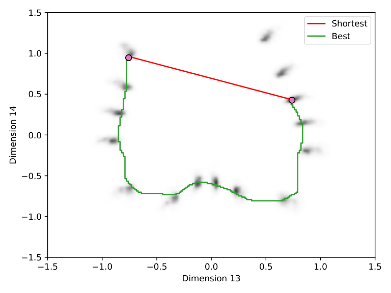
From the mean curvature response map in figure 5(a), we see that the manifold is particularly nonlinear along these two latent dimensions (13 and 14). Consequently, there can be a dramatic difference between the geodesic (here approximated using the mean curvature), compared to the shortest path in euclidean space as seen in figure 5.

Name	CDS	DCI-D	IRS	MIG
1-VAE	0.44	0.3	0.44	0.07
2-VAE	0.49	0.36	0.46	0.09
4-VAE	0.58	0.46	0.51	0.16
8-VAE	0.71	0.66	0.63	0.21
1-VAE	0.52	0.49	0.48	0.09
2-VAE	0.61	0.58	0.52	0.15
4-VAE	0.72	0.67	0.57	0.17
8-VAE	0.78	0.73	0.64	0.2

Table 1: Comparing disentanglement metrics for

\beta

-VAEs trained on 3D-shapes with varying

\beta

. For the models in the first four rows

d=12

, while

d=24

for the remaining four. While the CDS generally correlates well with other metrics, notably, the DCI-D score is consistently slightly lower which may be due to spurious correlations between latent variables and the true factors.

Causal Disentanglement

Table 1, unsurprisingly, shows the disentanglement increasing with increasing $\beta$ . Our proposed CDS score correlates strongly with the other disentanglement metrics. Perhaps noteworthy is that even though the CDS and DCI-D scores are computed in similar ways (the vital difference being whether responsibility rests on a causal link or a statistical correlation), the DCI-D scores are consistently lower than the CDS scores. This may be explained by the DCI-D metric taking additional spurious correlations between latent variables into account (as seen in figure 6), while the CDS metric focuses on the causal links, so the DCI-D has an undeservedly low score.

Causal Structure

Closer comparison between the conditioned response matrices and the responsibility matrices reveal more how the DCI-D metric and CDS differ. Figure 6 shows the responsibility matrix matches the conditioned response matrix for the most part. The only exception being latent variables 4 and 20. Since the DCI framework identifies which latent variables are most predictive for the true factors, it cannot distinguish between a correlation and a causal link. In this case, the DCI metric recognized a correlation between dimension 4 and the "scale" factor. However, from the latent response matrix (and the graph 6(d)) we see interventions on dim 20 have a significant effect on dim 4, but not vice versa. Consequently, we identify dim 20 is a parent of dim 4 in the learned causal graph. Since dim 20 is closely related with the "scale" factor the causal link to dim 4 results in dim 4 being correlated with "scale". The conditioned response matrix correctly identifies that it is dimension 20 which primarily affects the scale, but indirectly also affects the shape through dimension 4. This is a prime example of how causal reasoning can avoid misattributing responsibility due to spurious correlations.

6 Conclusion

In this work, we have introduced and motivated the latent response framework including a variety of tools to better visualize and understand the representations learned by variational autoencoders. Given an intervention on a sample in the latent space, the latent response quantifies the degree to which that intervention affects the semantic information in the sample. Therefore, we can think of this analysis as leveraging the interventional consistency of a representation to study the geometric and causal structure therein. Notably, the current analysis relies on a certain degree of axis-aligned structure in the latent space, which makes these tools especially useful for understanding the structure of disentangled representation. Another limitation is that computing the latent response maps to, for example, improve interpolations, does not scale well for the large representations of high fidelity generative models [Vahdat and Kautz 2020]. Consequently, our experiments thus far have focused on synthetic datasets designed for evaluating disentanglement methods. However, latent responses do not require any ground truth label information, which is particularly promising for better understanding representations of real datasets and consequently speed up development of not just better performing representation learning techniques, but also more interpretable and trustworthy [Li et al. 2021] models.

Acknowledgements

This work was supported by the German Federal Ministry of Education and Research (BMBF): Tübingen AI Center, FKZ: 01IS18039B, and by the Machine Learning Cluster of Excellence, EXC number 2064/1 – Project number 390727645. The authors thank the International Max Planck Research School for Intelligent Systems (IMPRS-IS) for supporting Felix Leeb.

References

Rumelhart et al. [1985] David E Rumelhart, Geoffrey E Hinton, and Ronald J Williams. Learning internal representations by error propagation. Technical report, California Univ San Diego La Jolla Inst for Cognitive Science, 1985.
Ballard [1987] Dana H Ballard. Modular learning in neural networks. In AAAI, pages 279–284, 1987.
Kingma and Welling [2013] Diederik P Kingma and Max Welling. Auto-encoding variational bayes. arXiv preprint arXiv:1312.6114, 2013.
Razavi et al. [2019] Ali Razavi, Aaron van den Oord, and Oriol Vinyals. Generating diverse high-fidelity images with vq-vae-2. arXiv preprint arXiv:1906.00446, 2019.
Townsend et al. [2019] James Townsend, Tom Bird, and David Barber. Practical lossless compression with latent variables using bits back coding. arXiv preprint arXiv:1901.04866, 2019.
An and Cho [2015] Jinwon An and Sungzoon Cho. Variational autoencoder based anomaly detection using reconstruction probability. Special Lecture on IE, 2(1):1–18, 2015.
Li et al. [2015] Jiwei Li, Minh-Thang Luong, and Dan Jurafsky. A hierarchical neural autoencoder for paragraphs and documents. arXiv preprint arXiv:1506.01057, 2015.
Vahdat and Kautz [2020] Arash Vahdat and Jan Kautz. Nvae: A deep hierarchical variational autoencoder. Advances in Neural Information Processing Systems, 33:19667–19679, 2020.
Child [2020] Rewon Child. Very deep vaes generalize autoregressive models and can outperform them on images. arXiv preprint arXiv:2011.10650, 2020.
Han et al. [2022] Ligong Han, Sri Harsha Musunuri, Martin Renqiang Min, Ruijiang Gao, Yu Tian, and Dimitris Metaxas. Ae-stylegan: Improved training of style-based auto-encoders. In Proceedings of the IEEE/CVF Winter Conference on Applications of Computer Vision, pages 3134–3143, 2022.
Miladinović et al. [2021] Đorđe Miladinović, Aleksandar Stanić, Stefan Bauer, Jürgen Schmidhuber, and Joachim M Buhmann. Spatial dependency networks: Neural layers for improved generative image modeling. International Conference on Learning Representations (ICLR), 2021.
Kingma and Welling [2019] Diederik P Kingma and Max Welling. An introduction to variational autoencoders. arXiv preprint arXiv:1906.02691, 2019.
Bank et al. [2020] Dor Bank, Noam Koenigstein, and Raja Giryes. Autoencoders. arXiv preprint arXiv:2003.05991, 2020.
Girin et al. [2020] Laurent Girin, Simon Leglaive, Xiaoyu Bie, Julien Diard, Thomas Hueber, and Xavier Alameda-Pineda. Dynamical variational autoencoders: A comprehensive review. arXiv preprint arXiv:2008.12595, 2020.
Bengio et al. [2012] Yoshua Bengio, Aaron Courville, and Pascal Vincent. Representation learning: A review and new perspectives, 2012. URL arXiv:1206.5538.
Dittadi et al. [2020] Andrea Dittadi, Frederik Träuble, Francesco Locatello, Manuel Wüthrich, Vaibhav Agrawal, Ole Winther, Stefan Bauer, and Bernhard Schölkopf. On the transfer of disentangled representations in realistic settings. arXiv preprint arXiv:2010.14407, 2020.
Srinivas et al. [2020] Aravind Srinivas, Michael Laskin, and Pieter Abbeel. Curl: Contrastive unsupervised representations for reinforcement learning. arXiv preprint arXiv:2004.04136, 2020.
Schott et al. [2021] Lukas Schott, Julius von Kügelgen, Frederik Träuble, Peter Gehler, Chris Russell, Matthias Bethge, Bernhard Schölkopf, Francesco Locatello, and Wieland Brendel. Visual representation learning does not generalize strongly within the same domain. arXiv preprint arXiv:2107.08221, 2021.
Locatello et al. [2018] Francesco Locatello, Stefan Bauer, Mario Lucic, Gunnar Rätsch, Sylvain Gelly, Bernhard Schölkopf, and Olivier Bachem. Challenging common assumptions in the unsupervised learning of disentangled representations. arXiv preprint arXiv:1811.12359, 2018.
Chen et al. [2018a] Ricky TQ Chen, Xuechen Li, Roger Grosse, and David Duvenaud. Isolating sources of disentanglement in variational autoencoders. arXiv preprint arXiv:1802.04942, 2018a.
Mathieu et al. [2019] Emile Mathieu, Tom Rainforth, Nana Siddharth, and Yee Whye Teh. Disentangling disentanglement in variational autoencoders. In International Conference on Machine Learning, pages 4402–4412. PMLR, 2019.
Liu et al. [2020] Wenqian Liu, Runze Li, Meng Zheng, Srikrishna Karanam, Ziyan Wu, Bir Bhanu, Richard J Radke, and Octavia Camps. Towards visually explaining variational autoencoders. In Proceedings of the IEEE/CVF Conference on Computer Vision and Pattern Recognition, pages 8642–8651, 2020.
Schölkopf et al. [2021] Bernhard Schölkopf, Francesco Locatello, Stefan Bauer, Nan Rosemary Ke, Nal Kalchbrenner, Anirudh Goyal, and Yoshua Bengio. Toward causal representation learning. Proceedings of the IEEE, 109(5):612–634, 2021.
Yang et al. [2021] Mengyue Yang, Furui Liu, Zhitang Chen, Xinwei Shen, Jianye Hao, and Jun Wang. Causalvae: Disentangled representation learning via neural structural causal models. In Proceedings of the IEEE/CVF Conference on Computer Vision and Pattern Recognition, pages 9593–9602, 2021.
Arvanitidis et al. [2017] Georgios Arvanitidis, Lars Kai Hansen, and Søren Hauberg. Latent space oddity: on the curvature of deep generative models. arXiv preprint arXiv:1710.11379, 2017.
Yang et al. [2018] Tao Yang, Georgios Arvanitidis, Dongmei Fu, Xiaogang Li, and Søren Hauberg. Geodesic clustering in deep generative models. arXiv preprint arXiv:1809.04747, 2018.
Connor et al. [2021] Marissa Connor, Gregory Canal, and Christopher Rozell. Variational autoencoder with learned latent structure. In International Conference on Artificial Intelligence and Statistics, pages 2359–2367. PMLR, 2021.
Chadebec et al. [2020] Clément Chadebec, Clément Mantoux, and Stéphanie Allassonnière. Geometry-aware hamiltonian variational auto-encoder. arXiv preprint arXiv:2010.11518, 2020.
Chen et al. [2020] Nutan Chen, Alexej Klushyn, Francesco Ferroni, Justin Bayer, and Patrick Van Der Smagt. Learning flat latent manifolds with vaes. arXiv preprint arXiv:2002.04881, 2020.
Kalatzis et al. [2021] Dimitris Kalatzis, Johan Ziruo Ye, Jesper Wohlert, and Søren Hauberg. Multi-chart flows. arXiv preprint arXiv:2106.03500, 2021.
Michelis and Becker [2021] Mike Yan Michelis and Quentin Becker. On linear interpolation in the latent space of deep generative models. arXiv preprint arXiv:2105.03663, 2021.
Rey et al. [2019] Luis A Pérez Rey, Vlado Menkovski, and Jacobus W Portegies. Diffusion variational autoencoders. arXiv preprint arXiv:1901.08991, 2019.
Chen et al. [2018b] Nutan Chen, Alexej Klushyn, Richard Kurle, Xueyan Jiang, Justin Bayer, and Patrick Smagt. Metrics for deep generative models. In International Conference on Artificial Intelligence and Statistics, pages 1540–1550. PMLR, 2018b.
Bronstein et al. [2017] Michael M Bronstein, Joan Bruna, Yann LeCun, Arthur Szlam, and Pierre Vandergheynst. Geometric deep learning: going beyond euclidean data. IEEE Signal Processing Magazine, 34(4):18–42, 2017.
Monti et al. [2017] Federico Monti, Davide Boscaini, Jonathan Masci, Emanuele Rodola, Jan Svoboda, and Michael M Bronstein. Geometric deep learning on graphs and manifolds using mixture model cnns. In Proceedings of the IEEE conference on computer vision and pattern recognition, pages 5115–5124, 2017.
Louizos et al. [2015] Christos Louizos, Kevin Swersky, Yujia Li, Max Welling, and Richard Zemel. The variational fair autoencoder. arXiv preprint arXiv:1511.00830, 2015.
Locatello et al. [2019] Francesco Locatello, Gabriele Abbati, Thomas Rainforth, Stefan Bauer, Bernhard Schölkopf, and Olivier Bachem. On the fairness of disentangled representations. In Advances in Neural Information Processing Systems, pages 14584–14597, 2019.
Ker et al. [2017] Justin Ker, Lipo Wang, Jai Rao, and Tchoyoson Lim. Deep learning applications in medical image analysis. Ieee Access, 6:9375–9389, 2017.
Chen et al. [2018c] Xiaoran Chen, Nick Pawlowski, Martin Rajchl, Ben Glocker, and Ender Konukoglu. Deep generative models in the real-world: An open challenge from medical imaging. arXiv preprint arXiv:1806.05452, 2018c.
Rezende et al. [2014] Danilo Jimenez Rezende, Shakir Mohamed, and Daan Wierstra. Stochastic backpropagation and approximate inference in deep generative models. arXiv preprint arXiv:1401.4082, 2014.
van Steenkiste et al. [2019] Sjoerd van Steenkiste, Francesco Locatello, Jürgen Schmidhuber, and Olivier Bachem. Are disentangled representations helpful for abstract visual reasoning? In Advances in Neural Information Processing Systems, 2019.
Eastwood and Williams [2018] Cian Eastwood and Christopher KI Williams. A framework for the quantitative evaluation of disentangled representations. 2018.
Shu et al. [2019] Rui Shu, Yining Chen, Abhishek Kumar, Stefano Ermon, and Ben Poole. Weakly supervised disentanglement with guarantees. arXiv preprint arXiv:1910.09772, 2019.
Whitney et al. [2020] William F Whitney, Min Jae Song, David Brandfonbrener, Jaan Altosaar, and Kyunghyun Cho. Evaluating representations by the complexity of learning low-loss predictors. arXiv preprint arXiv:2009.07368, 2020.
Tomczak and Welling [2018] Jakub Tomczak and Max Welling. Vae with a vampprior. In International Conference on Artificial Intelligence and Statistics, pages 1214–1223. PMLR, 2018.
Sinha et al. [2021] Abhishek Sinha, Jiaming Song, Chenlin Meng, and Stefano Ermon. D2c: Diffusion-decoding models for few-shot conditional generation. Advances in Neural Information Processing Systems, 34, 2021.
White [2016] Tom White. Sampling generative networks. arXiv preprint arXiv:1609.04468, 2016.
Yu and Principe [2019] Shujian Yu and Jose C Principe. Understanding autoencoders with information theoretic concepts. Neural Networks, 117:104–123, 2019.
Zhao et al. [2017] Shengjia Zhao, Jiaming Song, and Stefano Ermon. InfoVAE: Information maximizing variational autoencoders. arXiv preprint arXiv:1706.02262, 2017.
Lucas et al. [2019] James Lucas, George Tucker, Roger Grosse, and Mohammad Norouzi. Understanding posterior collapse in generative latent variable models. 2019.
Rezende and Viola [2018] Danilo Jimenez Rezende and Fabio Viola. Taming VAEs. arXiv preprint arXiv:1810.00597, 2018.
Cemgil et al. [2019] Taylan Cemgil, Sumedh Ghaisas, Krishnamurthy Dj Dvijotham, and Pushmeet Kohli. Adversarially robust representations with smooth encoders. In International Conference on Learning Representations, 2019.
Leeb et al. [2020] Felix Leeb, Guilia Lanzillotta, Yashas Annadani, Michel Besserve, Stefan Bauer, and Bernhard Schölkopf. Structure by architecture: Disentangled representations without regularization. arXiv preprint arXiv:2006.07796, 2020.
Cemgil et al. [2020] A Taylan Cemgil, Sumedh Ghaisas, Krishnamurthy Dvijotham, Sven Gowal, and Pushmeet Kohli. Autoencoding variational autoencoder. arXiv preprint arXiv:2012.03715, 2020.
Da Cruz et al. [2022] Steve Dias Da Cruz, Bertram Taetz, Thomas Stifter, and Didier Stricker. Autoencoder attractors for uncertainty estimation. arXiv preprint arXiv:2204.00382, 2022.
Zhang et al. [2020] Zijun Zhang, Ruixiang Zhang, Zongpeng Li, Yoshua Bengio, and Liam Paull. Perceptual generative autoencoders. In International Conference on Machine Learning, pages 11298–11306. PMLR, 2020.
Lanzillotta et al. [2021] Giulia Lanzillotta, Felix Leeb, Stefan Bauer, and Bernhard Schölkopf. On the interventional consistency of autoencoders. 2021.
Rifai et al. [2011] Salah Rifai, Pascal Vincent, Xavier Muller, Xavier Glorot, and Yoshua Bengio. Contractive auto-encoders: Explicit invariance during feature extraction. In Icml, 2011.
Radhakrishnan et al. [2018] Adityanarayanan Radhakrishnan, Karren Yang, Mikhail Belkin, and Caroline Uhler. Memorization in overparameterized autoencoders. arXiv preprint arXiv:1810.10333, 2018.
Dai and Wipf [2019] Bin Dai and David Wipf. Diagnosing and enhancing VAE models. arXiv preprint arXiv:1903.05789, 2019.
Stühmer et al. [2020] Jan Stühmer, Richard Turner, and Sebastian Nowozin. Independent subspace analysis for unsupervised learning of disentangled representations. In International Conference on Artificial Intelligence and Statistics, pages 1200–1210. PMLR, 2020.
Hoffman and Johnson [2016] Matthew D Hoffman and Matthew J Johnson. Elbo surgery: yet another way to carve up the variational evidence lower bound. In Workshop in Advances in Approximate Bayesian Inference, NIPS, volume 1, 2016.
Sitzmann et al. [2020] Vincent Sitzmann, Julien Martel, Alexander Bergman, David Lindell, and Gordon Wetzstein. Implicit neural representations with periodic activation functions. Advances in Neural Information Processing Systems, 33:7462–7473, 2020.
Genova et al. [2019] Kyle Genova, Forrester Cole, Daniel Vlasic, Aaron Sarna, William T Freeman, and Thomas Funkhouser. Learning shape templates with structured implicit functions. In Proceedings of the IEEE/CVF International Conference on Computer Vision, pages 7154–7164, 2019.
Theisel [1995] Holger Theisel. Vector field curvature and applications. PhD thesis, 1995.
Burgess and Kim [2018] Chris Burgess and Hyunjik Kim. 3d shapes dataset, 2018.
LeCun et al. [1998] Yann LeCun, Léon Bottou, Yoshua Bengio, and Patrick Haffner. Gradient-based learning applied to document recognition. Proceedings of the IEEE, 86(11):2278–2324, 1998.
Xiao et al. [2017] Han Xiao, Kashif Rasul, and Roland Vollgraf. Fashion-mnist: a novel image dataset for benchmarking machine learning algorithms. arXiv preprint arXiv:1708.07747, 2017.
Kingma and Ba [2014] Diederik P Kingma and Jimmy Ba. Adam: A method for stochastic optimization. arXiv preprint arXiv:1412.6980, 2014.
Burgess et al. [2018] Christopher P Burgess, Irina Higgins, Arka Pal, Loic Matthey, Nick Watters, Guillaume Desjardins, and Alexander Lerchner. Understanding disentangling in $\beta$ -VAE. arXiv preprint arXiv:1804.03599, 2018.
Li et al. [2021] Bo Li, Peng Qi, Bo Liu, Shuai Di, Jingen Liu, Jiquan Pei, Jinfeng Yi, and Bowen Zhou. Trustworthy ai: From principles to practices. ArXiv, abs/2110.01167, 2021.
[72] Cian Eastwood, Andrei Liviu Nicolicioiu, Julius Von Kügelgen, Armin Kekic, Frederik Träuble, Andrea Dittadi, and Bernhard Schölkopf. On the dci framework for evaluating disentangled representations: Extensions and connections to identifiability. In UAI 2022 Workshop on Causal Representation Learning.
Bengio et al. [2013] Yoshua Bengio, Aaron Courville, and Pascal Vincent. Representation learning: A review and new perspectives. IEEE transactions on pattern analysis and machine intelligence, 35(8):1798–1828, 2013.
Arvanitidis et al. [2019] Georgios Arvanitidis, Soren Hauberg, Philipp Hennig, and Michael Schober. Fast and robust shortest paths on manifolds learned from data. In The 22nd International Conference on Artificial Intelligence and Statistics, pages 1506–1515. PMLR, 2019.
Kalatzis et al. [2020] Dimitris Kalatzis, David Eklund, Georgios Arvanitidis, and Søren Hauberg. Variational autoencoders with riemannian brownian motion priors. arXiv preprint arXiv:2002.05227, 2020.
Davidson et al. [2018] Tim R Davidson, Luca Falorsi, Nicola De Cao, Thomas Kipf, and Jakub M Tomczak. Hyperspherical variational auto-encoders. arXiv preprint arXiv:1804.00891, 2018.
Falorsi et al. [2018] Luca Falorsi, Pim de Haan, Tim R Davidson, Nicola De Cao, Maurice Weiler, Patrick Forré, and Taco S Cohen. Explorations in homeomorphic variational auto-encoding. arXiv preprint arXiv:1807.04689, 2018.
Lin and Zha [2008] Tong Lin and Hongbin Zha. Riemannian manifold learning. IEEE Transactions on Pattern Analysis and Machine Intelligence, 30(5):796–809, 2008.
Tosi et al. [2014] Alessandra Tosi, Søren Hauberg, Alfredo Vellido, and Neil D Lawrence. Metrics for probabilistic geometries. arXiv preprint arXiv:1411.7432, 2014.

Appendix A Appendix

A.1 Latent Responses

In a similar setup as Cemgil et al. 2020, we can extend the joint distribution $p(X,Z)$ to include the reconstruction and response as $p(X,Z,\hat{X},\hat{Z})$ , where crucial question is how the posterior $q(Z\,|\,X;\phi)$ relates to the response $q(\hat{Z}\,|\,\hat{X};\phi)$ where $Z$ and $\hat{Z}$ are related by (also shown in equation 7):

r(\hat{Z}\,|\,Z;\theta,\phi)=\int q(\hat{Z}\,|\,\hat{X};\phi)p(\hat{X}\,|\,Z;\theta)\mathrm{d}\hat{X}

(12)

Note, that $r(\hat{Z}\,|\,Z;\theta,\phi)$ is equivalent to the transition kernel $\mathcal{Q}_{\mathrm{AVAE}}$ in Cemgil et al. 2020. However, crucially, we do not make two assumptions used to derive the AVAE objective. Firstly, we do not assume that the decoder is a one-to-one mapping between latent samples and a corresponding generated sample. The contractive behavior observed in the latent space of autoencoders [Radhakrishnan et al. 2018], suggests a many-to-one mapping is more realistic, which may be interpretted as the decoder filtering out useless exogenous information from the latent code. Consequently, we also do not treat $p(\hat{Z};\theta,\phi)=\mathbb{E}_{p(Z)}[r(\hat{Z}\,|\,Z;\theta,\phi)]$ as a normal distribution, which would imply the encoder perfectly inverts the decoder.

Consider the reconstructions $\hat{X}$ of the maximally overfit encoder $q(z=Z\,|\,x_{i}=X;\tilde{\phi})=\delta(s_{i}-z)$ (recall $s_{i}=f^{\phi}(x_{i})$ ) and decoder $p(\hat{X}\,|\,Z;\tilde{\theta})$ . Since the autoencoder is trained on the empirical generative process $\pi(X)$ rather than the true generative process $p(X)$ , the overfit decoder generates samples from $p(\hat{X};\tilde{\theta})=\int p(\hat{X}\,|\,Z;\tilde{\theta})p(Z)\mathrm{d}Z=\pi(X)$ , which does not have continuous support. For such a decoder, all exogenous noise is completely removed and the decoder mapping is obviously many-to-one, and it follows that $r(\hat{Z}=\hat{z}\,|\,Z=z;\tilde{\theta},\tilde{\phi})=\delta(\hat{z}-s)$ (recall $z=s+u$ ).

Now consider the more desirable (and perhaps slightly more realistic) setting where the autoencoder extrapolates somewhat beyond $\pi(X)$ to resemble $p(X)$ , in which case decoding the latent sample $z\sim q(Z\,|\,X=x;\phi)$ to generate $\hat{x}\sim p(\hat{x}=\hat{X}\,|\,z=Z;\theta)$ will not necessarily match the observation $x$ , which, by our definition of endogenous information, implies a change in the endogenous information contained in $z$ . When re-encoding to get $q(\hat{Z}\,|\,\hat{X}=\hat{x};\phi)$ , the changes in the endogenous information result in some width to the distribution over $\hat{Z}$ .

A.2 Derivation of Equation 6

Starting from our definition of $\hat{s}=f^{\phi}(\hat{x})$ where $\hat{x}=g^{\theta}(z)$ , $z=f^{\phi}(x)$ , $z=s+u$ , and $\epsilon=\hat{x}-x$ .

The high-level goal is expand $f^{\phi}$ around $x$ and then $g^{\theta}$ around $s$ to first order.

\hat{s}=f^{\phi}(\hat{x})

\hat{s}=f^{\phi}(x+\epsilon)

\hat{s}=f^{\phi}(x)+\mathbf{J}_{f^{\phi}}(x)\epsilon+\mathcal{O}\left[\epsilon^{2}\right]

\hat{s}=f^{\phi}(x)+\mathbf{J}_{f^{\phi}}(x)\left[g^{\theta}(z)-x\right]+\mathcal{O}\left[\epsilon^{2}\right]

\hat{s}=f^{\phi}(x)+\mathbf{J}_{f^{\phi}}(x)\left[g^{\theta}(s+u)-x\right]+\mathcal{O}\left[\epsilon^{2}\right]

\hat{s}=f^{\phi}(x)+\mathbf{J}_{f^{\phi}}(x)\left[g^{\theta}(s)+\mathbf{J}_{g^{\theta}}(s)u-x\right]+\mathcal{O}\left[\epsilon^{2}\right]+\mathcal{O}\left[u^{2}\right]

\hat{s}=f^{\phi}(x)+\mathbf{J}_{f^{\phi}}(x)(g^{\theta}(s)-x)+\mathbf{J}_{f^{\phi}}(x)\mathbf{J}_{g^{\theta}}(s)u+\mathcal{O}\left[\epsilon^{2}\right]+\mathcal{O}\left[u^{2}\right]

A.3 Comparing the Conditioned Response Matrix and the DCI Responsibility Matrix

In Eastwood and Williams 2018, the responsibility matrix is used to evaluate the disentanglement of a learned representation. In the matrix, element $R_{ij}$ corresponds to the relative importance of latent variable $j$ in predicting the true factor of variation $i$ for a simple classifier trained with full supervision to recover the true factors from the latent vector. Although the scalar scores (DCI-d and CDS) are computed identically from the respective matrices, there are important practical and theoretical distinctions in the DCI and latent response frameworks.

First and most importantly, since the DCI framework only uses the encoder, the learned generative process is not taken into account at all. Consequently, the DCI framework (and other existing disentanglement metrics) fail to evaluate how disentangled the causal drivers of the learned generative process are, and instead evaluate which latent variables are correlated with true factors. Furthermore, practically speaking, the DCI framework is sensitive to a variety of hyperparameters such as the exact design and training of the model [Eastwood et al.], while the conditioned response matrix has far fewer (and more intuitive) hyperparameters relating to the Monte carlo integration.

Interestingly, the DCI responsibility matrices do often resemble the conditioned response matrices, suggesting that relying on correlations instead of a full causal analysis, can yield similar results. Obviously as the data becomes more challenging and realistic, and the true generative process involves a more complicated causal structure, then we may expect the DCI responsibility matrix to become less reliable for analyzing the generative model structure. In fact, then the learned causal structure estimated using the latent response matrix may be used in tandem to develop a structure-aware disentanglement metric.

A.4 Mean Curvature for Manifold Learning

The geometry of learned representations with a focus on the generalization ability of neural networks has been discussed in [Bengio et al. 2013]. One key problem is that the standard Gaussian prior used in variational autoencoders relies on the usual Lebesgue measure which in turn, assumes a Euclidean structure over the latent space. This has been demonstrated to lead to difficulties in particular when interpolating in the latent space [Arvanitidis et al. 2017, Arvanitidis et al. 2019, Kalatzis et al. 2020] due to a manifold mismatch [Davidson et al. 2018, Falorsi et al. 2018]. Given the complexity of the underlying data manifold, a viable alternative is based on riemanian geometry [Lin and Zha 2008] which has previously been investigated for alternative probabilistic models like Gaussian Process regression [Tosi et al. 2014].

These methods focus on the intrinsic curvature of the data manifold, which does not depend on the specific embedding of the manifold in the latent space. However, our focus is precisely on how the data manifold is embedded in the latent space, to (among other things) quantify the relationships between latent variables and how well the representation disentangles the true factors of variation. Consequently, we focus on the extrinsic curvature, and more specifically the mean curvature which can readily be estimated using the response maps.

As discussed in the main paper, $|u(z)|=|z-s|$ is interpreted as a distance where $|u(z)|=0$ implies $z$ is on the latent manifold and there is no exogenous noise. The gradient of this function $\nabla_{z}|u(z)|$ , effectively projects any point in the latent space onto the endogenous manifold. Similarly, the mean curvature (equation 13) can be computed, which can be interpreted as identifying the regions in the latent space where the $|u(z)|$ converges and diverges. These gradients are estimated numerically by finite differencing.

H=-\frac{1}{2}\nabla_{z}\cdot\left(\frac{\nabla_{z}|u(z)|}{|\nabla_{z}|u(z)||}\right)=-\frac{1}{2}\nabla_{z}\cdot\frac{u(z)}{|u(z)|}

(13)

A.5 Double Helix Example Details

x_{i}=\left[A_{1}\cos(\pi(\omega t_{i}+n_{i})),A_{2}\sin(\pi(\omega t_{i}+n_{i})),A_{3}t_{i}\right]^{T}+\epsilon_{i}

(14)

where $t_{i}\sim\mathrm{Uniform}(-1,1)$ , $n_{i}\sim\mathrm{Bernoulli}(0.5)$ , $\epsilon_{i}\sim\mathcal{N}(\mathbf{0},\sigma\mathbf{I})$ . For this experiment, we set $A_{1}=A_{2}=A_{3}=\omega=1$ and $\sigma=0.1$ .

Disregarding the additive noise $\epsilon_{i}$ , the data manifold has two degrees of freedom, which are the strand location $t_{i}$ and the strand number $n_{i}$ .

To provide the model sufficient capacity, we use four hidden layers with 32 units each for the encoder and decoder. We train until convergence (at most 5k steps) with $\beta$ = 0.05 using an Adam optimizer on a total of $N=1024$ training samples (see the supplementary code for the full training and evaluation details).

Figure 7: The response map of the representation trained on the double helix. Starting from the latent samples (blue dots), applying the decoder followed by the encoder (i.e. response function) results in the orange dots connected by the black arrows. Note that applying the response function effectively contracts points all over the latent space into a relatively small non-linear region, corresponding to endogenous information.

A.6 Architecture and Training Details

All our models are based on the same convolutional neural network architecture detailed in table 10 so that in total models have approximately 500k trainable parameters. For the smaller datasets MNIST and Fashion-MNIST, samples are upsampled to 32x32 pixels from their original 28x28 and the one convolutional block is removed from both the encoder and decoder.

The datasets are split into a 70-10-20 train-val-test split, and are optimized using Adam Kingma and Ba 2014 with a learning rate of 0.0001, weight decay 0, and $\beta_{1}$ , $\beta_{2}$ of 0.9 and 0.999 respectively. The models are trained for 100k iterations with a batch size of 64 (128 for MNIST and Fashion-MNIST).

Input 64x64x3 image
Conv Layer (64 filters, k=5x5, s=1x1, p=2x2)
Max pooling (filter 2x2, s=2x2)
Group Normalization (8 groups, affine)
ELU activation
Conv Layer (64 filters, k=3x3, s=1x1, p=1x1)
Max pooling (filter 2x2, s=2x2)
Group Normalization (8 groups, affine)
ELU activation
Conv Layer (64 filters, k=3x3, s=1x1, p=1x1)
Max pooling (filter 2x2, s=2x2)
Group Normalization (8 groups, affine)
ELU activation
Conv Layer (64 filters, k=3x3, s=1x1, p=1x1)
Max pooling (filter 2x2, s=2x2)
Group Normalization (8 groups, affine)
ELU activation
Conv Layer (64 filters, k=3x3, s=1x1, p=1x1)
Max pooling (filter 2x2, s=2x2)
Group Normalization (8 groups, affine)
ELU activation
Fully-connected Layer (256 units)
ELU activation
Fully-connected Layer (128 units)
ELU activation
Fully-connected Layer ( $2d$ units)
Output posterior $\mu$ and $\log\sigma$

Figure 8: Encoder Architecture

Input $d$ latent vector
Fully-connected Layer (128 units)
ELU activation
Fully-connected Layer (256 units)
ELU activation
Fully-connected Layer (256 units)
ELU activation
Bilinear upsampling (scale 2x2)
Conv Layer (64 filters, k=3x3, s=1x1, p=1x1)
Group Normalization (8 groups, affine)
ELU activation
Bilinear upsampling (scale 2x2)
Conv Layer (64 filters, k=3x3, s=1x1, p=1x1)
Group Normalization (8 groups, affine)
ELU activation
Bilinear upsampling (scale 2x2)
Conv Layer (64 filters, k=3x3, s=1x1, p=1x1)
Group Normalization (8 groups, affine)
ELU activation
Bilinear upsampling (scale 2x2)
Conv Layer (64 filters, k=3x3, s=1x1, p=1x1)
Group Normalization (8 groups, affine)
ELU activation
Conv Layer (3 filters, k=3x3, s=1x1, p=1x1)
Sigmoid activation
Output 64x64x3 image

Figure 9: Decoder Architecture

Figure 10: Model architectures where "k" is the kernel size, "s" is the stride, and "p" is the zero-padding

Appendix B Additional Results

B.1 3D-Shapes

B.2 MPI3D

Name	CDS	DCI-D	IRS	MIG
1-VAE	0.69	0.33	0.58	0.32
2-VAE	0.86	0.17	0.59	0.14
4-VAE	0.66	0.11	0.61	0.05
8-VAE	1	0.13	0.79	0.1
1-VAE	0.61	0.24	0.51	0.07
2-VAE	0.69	0.26	0.72	0.24
4-VAE	0.4	0.09	0.75	0.04
8-VAE	0.7	0.08	0.71	0.04

Table 2: disentanglement scores for the MPI3D Toy (first four rows) and Real (last four rows).

B.3 MNIST

Due to the computational cost of evaluating the response function over a dense grid, we focus our visualizations to 2D projections of the latent space. However, for MNIST and Fashion-MNIST, we train several VAE models to embed the whole representation into two dimensions $d=2$ , so that we can visualize the full representation. While the resulting divergence and curvature maps do not demonstrate as intuitive structure as in the disentangled representations for 3D-Shapes or MPI-3D, we can nevertheless appreciate the learned manifold beyond qualitatively observing reconstructions.

B.3.1 MNIST

(a) Response field

[-2,2]

(b) Response field

[-4,4]

Figure 28: Response fields for the same model analyzed in figures 26 and 27. The blue dots show the initial latent samples, and the orange dots connected by the black arrows show the corresponding responses (the latent sample after decoding and reencoding).

B.3.2 Fashion-MNIST

(a) Response field

[-2,2]

(b) Response field

[-4,4]

Figure 31: Response fields for the same model analyzed in figures 29 and 30. The blue dots show the initial latent samples, and the orange dots connected by the black arrows show the corresponding responses (the latent sample after decoding and reencoding).