Burling graphs revisited,
part II: Structure

Graphs in this paper have neither loops nor multiple edges. In this introduction they are non-oriented, but oriented graphs will sometimes be considered in the rest of the paper. A class of graphs is hereditary if it is closed under taking induced subgraphs. A triangle in a graph is a set of three pairwise adjacent vertices, and a graph is triangle-free if it contains no triangle.

In 1965, Burling [2] proved that triangle-free intersection graphs of axis-parallel boxes in $\mathbb{R}^{3}$ have unbounded chromatic number. The work of Burling uses geometric terminology. However, one may rephrase it into a more modern graph theoretic setting by defining in a combinatorial way a sequence of triangle-free graphs, called the Burling sequence, with increasing chromatic number, and proving that each of them is isomorphic to the intersection graph of a set of axis-parallel boxes in $\mathbb{R}^{3}$. It was later proved that every graph in the Burling sequence is isomorphic to the intersection graph of various geometrical objects, see [3, 8, 9, 11].

The Burling sequence also attracted attention lately because it is a good source of non-$\chi$-bounded classes of graphs. Let us explain this. A heredatiry class of graphs is $\chi$-bounded if there exists a function $f$ such that for every graph $G$ in the class, $\chi(G)\leq f(\omega(G)$, where $\chi(G)$ denotes the chromatic number of $G$ and $\omega(G)$ the maximum number of pairwise adjacent vertices in $G$. In [8], it is shown that there exist graphs $H$ such that graphs in the Burling sequence (and therefore some triangle-free graphs with arbitrary large chromatic number) do not contain any subdivision of $H$ as an induced subgraph. This provides counter-examples to a well-studied conjecture of Scott (Conjecture 8 in [13]), saying that for every $H$, the class of graphs that do not contain any subdivision of $H$ as an induced subgraphs are $\chi$-bounded. A counter-example to Scott conjecture is called a non-weakly pervasive graph. Despite the fact that Scott’s conjecture is disproved in [8], classifying graphs into weakly pervasive and non-weakly pervasive remains of interest.

This paper is the second part in a series of three articles, so let us explain briefly the content of the other parts. In all the series, we call Burling graph any graph that is isomorphic to an induced subgraph of some graph in the Burling sequence. In the first part of this work [11], we give several equivalent definitions of Burling graphs, including geometrical characterizations. In the third part of this work [12], our goal is to use results from the previous parts to make progress toward understanding weakly pervasive graphs by giving new examples of graphs that are not weakly pervasive.

In this second part, we use one of the new equivalent definitions from the first part [11] (namely derived graphs) to study the structure of Burling graphs. Among other results, we give a decomposition theorem for oriented Burling graphs, characterize the subdivisions of $K_{4}$ that are Burling graphs, and give a new characterization of Burling graphs (called $k$-sequential graphs). We also answer some open questions in $\chi$-boundedness: an open problem of the second author in [16] and a conjecture of Scott and Seymour in [14] (both concerning wheel-free graphs). Moreover, most of the results in this part have applications in the third part [12] as well. We postpone the explanations for these applications to part III, and in the following brief outline of the paper, we explain how the structural results of this contribution are motivated in their own rights.

In section 2, we describe the notation that we use.

In section 3, we recall the definition of derived graphs (first defined in Part I of this work [11] where they are shown to be equivalent to Burling graphs) which are oriented graphs obtained from a tree by some precise rules. We also show how their arcs can be subdivided, providing generic constructions of Burling graphs. This study of subdivisions seems important to us, because the class of Burling graphs is so far the only source of non-weakly pervasive graphs.

In section 4, we define the notion of nobility of a Burling graph (roughly, it is the maximum number of vertices of the graph that lie in a branch of a tree from which the graph can be derived). We then show how Burling graphs of a given nobility can be constructed from graphs of smaller nobility. The section is mostly motivated by the need of the so-called 2-Burling graphs that serve as basic graphs in the decomposition theorem of the next section. We also present $k$-Burling graphs that enables us to provide another equivalent definition of Burling graphs.

In Section 5, we give a decomposition theorem for Burling graphs using star cutsets. This theorem was already proved by Chalopin, Esperet, Li and Ossona de Mendez in [3]. Our contribution is to give a stronger result for oriented Burling graphs that we need in this part (Section 6) and in part 3. Interestingly, star cutsets have been proved very useful in the proof of the strong perfect graph theorem. They were invented by Chváta [6]l who generalized them to skew partitions, and who proved that in some sense, star cutsets preserve being perfect. It is not the place here to give too much detail about that, but briefly speaking, many classes of perfect graphs, including the class of all perfect graphs, have decomposition theorems [5] (a graph in the class is basic or has a decomposition), and star cutsets or one of their variants (skew partitions, double star cutsets, etc.) are often one of the decompositions. It is therefore striking to see a class of triangle-free graphs of high chromatic number that can still be decomposed into very simple graphs by star cutsets. Moreover, we observe here for the first time that the decomposition theorem of Burling graphs in [3] disproves an open question from [4] about star cutset preserving in some sense bounds on the chromatic number. We believe that this explains why the decomposition method that was so efficient to prove the strong perfect graph theorem did not provide many results in the more general field of $\chi$-boundedness.

In section 6, we describe properties of holes in Burling graphs, where a hole is a chordless cycle of length at least 4. Results from this section provide essential tools for the proofs in Section 7 and for the results in part 3 of this work. In particular, the orientation of a hole in a Burling graph is used intensively in the sequel. Also, how a graph is organized regarding its holes is very often of interest in studying the structure of many classes of graphs, so we believe that our study might help future works about the structure of Burling graphs as well.

In section 7, using the results of our structural studies, we give several examples of graphs that are not Burling. Among these examples are wheels (graphs build from a hole and a vertex with at least three neighbors in that hole). This results proves that the class of wheel-free graphs is not $\chi$-bounded, which answers negatively a question of the second author in [16], and disproves a conjecture of Scott and Seymour in [15]. This result is independently proved by Davies [7] (with a different technique) and has been claimed by Scott and Seymour [14] in a personal communication. However, our proof, appearing first in the master’s thesis of the first author [10] is the first written proof of this theorem.

To sum up, besides answering some open problems, we study here many structural aspects of Burling graphs, most notably, their closure under subdivision, decomposition theorem, structure and holes. We believe that these studies, along with the examples we provide, might help solving the following questions.

We denote by $N(v)$ the neighborhood of $v$, and denote by $N[v]$ the closed neighborhood of $v$, that is $N(v)\cup\{v\}$. If the graph is oriented, $N^{-}(v)$ and $N^{+}(v)$ denote the set of in-neighbors and out-neighbors of $v$ respectively, and $N^{-}[v]$ and $N^{+}[v]$ are the closed versions of them.

There is a difficulty regarding notations in this paper. The graphs we are interested in will be defined from trees. More specifically, a tree $T$ is considered and a graph $G$ is derived from it by following some rules that are defined in the next section. We have $V(G)=V(T)$ but $E(G)$ and $E(T)$ are different (disjoint, in fact). Also, even if we are originally motivated by non-oriented graphs, it turns out that $G$ has a natural orientation, and considering it is essential in many of our proofs.

So, in many situations we have to deal simultaneously with the tree, the oriented graph derived from it and the underlying graph of this oriented graph. A last difficulty is that since we are interested in hereditary classes, we allow removing vertices from $G$. But we have to keep all vertices of $T$ to study $G$ because the so-called shadow vertices, the ones from $T$ that are not in $G$, capture essential structural properties of $G$. All this will be clearer in the next section. For now, it explains why we need to be very careful about the notation. For any classical notion that we do not define, refer to [1].

In this section, we recall the definition and main properties of derived graphs that were introduced in [11]. A Burling tree is a 4-tuple $(T,r,\lastBorn,\choosePath)$ in which:

1. (i)

   $T$ is a rooted tree and $r$ is its root,

2. (ii)

   $\lastBorn$ is a function associating to each vertex $v$ of $T$ which is not a leaf, one child of $v$ which is called the last-born of $v$,

3. (iii)

   $\choosePath$ is a function defined on the vertices of $T$. If $v$ is a non-last-born vertex of $T$ other than the root, then $\choosePath$ associates to $v$ the vertex-set of a (possibly empty) branch in $T$ starting at the last-born of $p(v)$. If $v$ is a last-born or the root of $T$, then we define $\choosePath(v)=\varnothing$. We call $\choosePath$ the choose function of $T$.

By abuse of notation, we often use $T$ to denote the 4-tuple.

The oriented graph $G$ fully derived from the Burling tree $T$ is the oriented graph whose vertex-set is $V(T)$ and such that $uv\in A(G)$ if and only if $v$ is a vertex in $\choosePath(u)$. A non-oriented graph $G$ is fully derived from $T$ if it is the underlying graph of the oriented graph fully derived from $T$.

A graph (resp. oriented graph) $G$ is derived from a Burling tree $T$ if it is an induced subgraph of a graph (resp. oriented graph) fully derived from $T$. The graph (resp. oriented graph) $G$ is called a derived graph if there exists a Burling tree $T$ such that $G$ is derived from $T$.

Observe that if the root of $T$ is in $V(G)$, then it is an isolated vertex of $G$. Observe that a last-born vertex of $T$ that is in $G$ is a sink of $G$. This does not mean that every oriented derived graph has a sink, because it could be that no last-born of $T$ is in $V(G)$.

In 1965, Burling [2] introduced a sequence $\{G_{k}\}_{k\geq 1}$ of graphs such that $\chi(G_{k})=k$ and where each $G_{k}$ is a triangle-free intersection graph of some boxes (i.e. axis parallel cuboids) in $\mathbb{R}^{3}$ (see [2] or [11] for the definition). The class of Burling graphs is the class of all induced subgraphs of the graphs in the sequence $\{G_{k}\}$. It was proved in [11] that a graph is a Burling graph if and only if it can be derived from a Burling tree (Theorem 4.9 of [9]). So in what follows, we use “Burling graph” or “graph derived from a tree” according to what is most convenient.

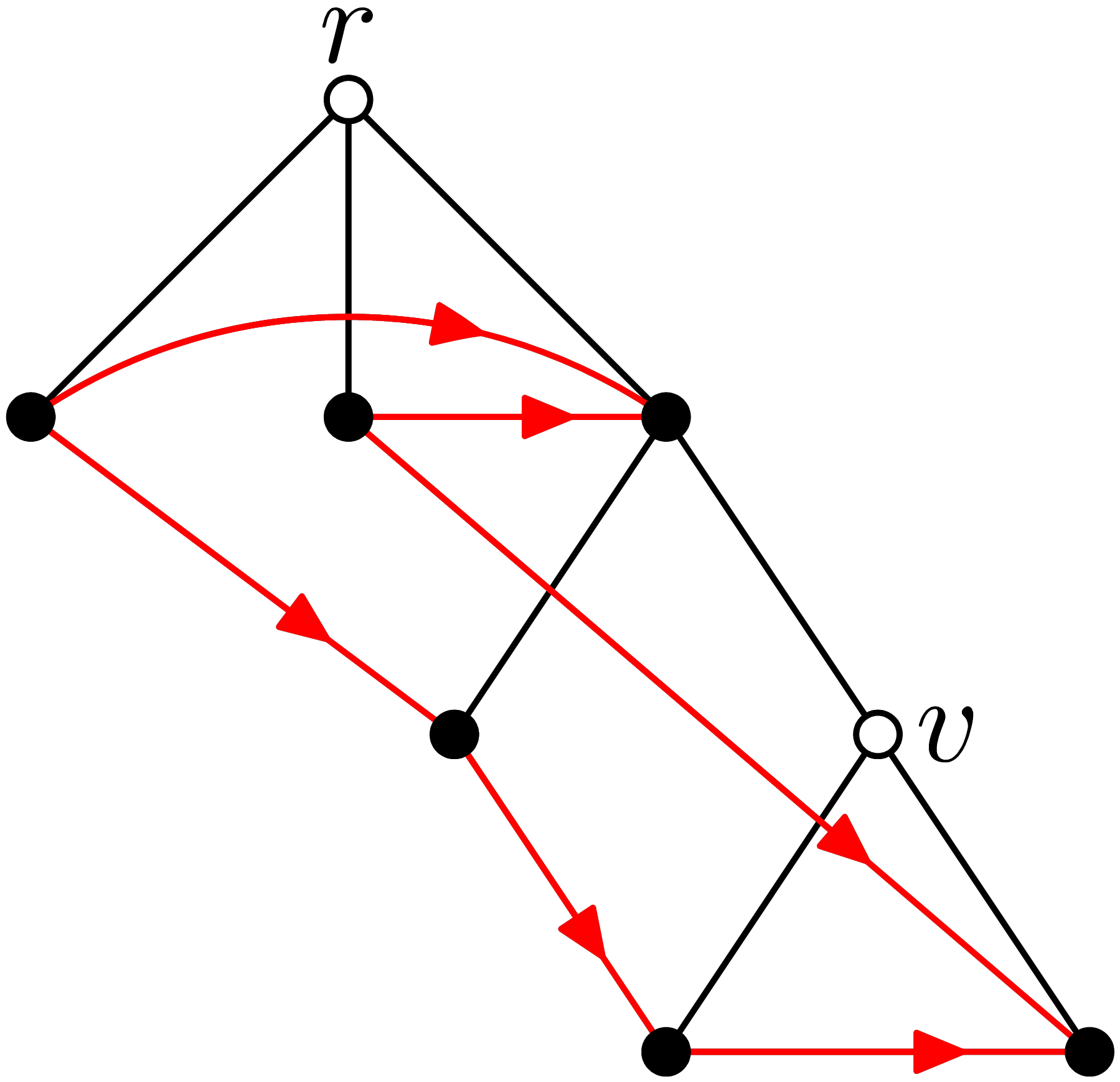
Now, let us give some examples of derived graphs. We use the convention in all figures in this paper that the tree $T$ is represented with black edges while the arcs of $G$ are represented in red. The last-born of a vertex of $T$ is its rightmost child. Moreover, denoting a vertex of $T$ in white means that this vertex in not in $G$.

In the first graph represented in Figure 1, we have $\choosePath(u)=\choosePath(v)=\{x,y\}$. It shows that there exists an orientation of $C_{4}$ which is an oriented derived graph, so $C_{4}$ is a derived graph. The second graph shows that $K_{3,3}$ is a derived graph, and it is easy to generalize this construction to $K_{n,m}$ for all integers $n,m\geq 1$. In both graphs, the vertex $r$ of $T$ is not a vertex of $G$. Figure 2 is a presentation of $C_{6}$ as a derived graph. Notice that in this presentation, the vertex $v$ is not in $G$.

Notice that if a graph $G$ is derived from $T$, the branches of $T$, restricted to the vertices of $G$, are stable sets of $G$. In particular, no edge of $T$ is an edge of $G$.

The next lemma shows that all oriented Burling graphs can be derived from Burling trees with specific properties. This will reduce complication in some proofs. Let $G$ be an oriented graph derived from a Burling tree $T$. An arc $uv$ of $G$ is a top-arc with respect to $T$ if $v$ is the out-neighbor of $u$ that is closest (in $T$) to the root of $T$. An arc $uv$ of $G$ is a bottom-arc with respect to $T$ if $v$ is the out-neighbor of $u$ that is furthest (in $T$) from the root of $T$. Note that it is possible that a top (resp. bottom) arc with respect to $T$ is no longer a top-arc (resp. bottom) when $G$ is derived from another tree $T^{\prime}$. This is why we add “with respect to $T$” but we omit it when $T$ is clear from the context. Informally, top-arcs and bottom-arcs are arcs that can be subdivided while preserving being Burling, as we will show in Lemma 3.8.

An oriented graph $G$ is a oriented $k$-Burling graph if it can be derived from a Burling tree $T$ such that on each branch of $T$, at most $k$ vertices belong to $G$. In such a case, we say that $G$ is derived from $T$ as a $k$-Burling graph. Note that the empty graph is the unique 0-Burling graph (in fact, the empty graph is $k$-Burling for all integers $k\geq 0$). In the next sections, 2-Burling graphs will be useful and we need to describe them more precisely. Since it is not much harder to describe $k$-Burling graphs in general, we do this here by the mean of the so-called $k$-sequential graphs.

The nobility of an oriented graph is the smallest integer $k$ such that $G$ is a $k$-Burling graph. The nobility of a non-oriented Burling graph $G$ is the smallest nobility of an oriented Burling graph $G^{\prime}$ such that $G$ is the underlying graph of $G^{\prime}$.

Let us see examples. On Figure 10, two oriented graphs $G_{1}$ and $G_{2}$ are represented. Since $G_{1}$ can be derived from $T_{1}$, we see that $G_{1}$ is a 2-Burling graph. In fact, the nobility of $G_{1}$ must be 2, because since $c$ is a source of degree 2, its two out-neighbors must be on the same branch. Similarly, $G_{2}$ is a 3-Burling graph and has nobility 3 (because of $y$ being a source of degree 3). Hence, $G$ is a 2-Burling graph (in fact it has nobility 2 because we will soon see that only forests have nobility 1). This shows that an oriented graph (for instance $G_{2}$) may have a nobility different from the nobility of its underlying graph.

In Figure 11, an oriented Burling graph $G$ with nobility 3 is represented together with two Burling graphs $T_{1}$ and $T_{2}$. Observe that $T_{2}$ has a branch that contains four vertices of $G$. So, $G$ is derived from $T_{1}$ as a 3-Burling graph, and is derived from $T_{2}$ as a 4-Burling graph.

It should be pointed out that the nobility of an oriented graph may be strictly greater than its maximum out-degree, as shown on Figure 12. The graph $G$ has three sources with out-neighborhood $\{1,2,3\}$, $\{2,3,4\}$ and $\{3,4,5\}$. Assume that $G$ is derived from a Burling tree $T$. At least four vertices among 1, 2, 3, 4 and 5 must lie on the same branch of $T$. We only sketch the proof: on the branch of $T$ that contains 1, 2, and 3, either 1 is the farthest vertex from the root or it is not. In the former case, if 4 is not a descendant of both 2 and 3, then 1, 2, 3, and 4 are all on a common branch, and if 4 is a descendant of both 2 and 3, then any branch containing 4, contains both 3, and 5. So, in particular, 2, 3, 4, and 5 are on a common branch. In the latter case (where 1 is not the farthest from root among 1, 2, and 3), any branch containing both 2 and 3 contains 1 as well. So, in particular 1, 2, 3, and 4 are on a common branch. So, the nobility of $G$ is 4.

References

- [1] John Adrian Bondy and Uppaluri Siva Ramachandra Murty. Graph Theory with Applications. Elsevier, New York, 1976.
- [2] James Perkins Burling. On coloring problems of families of polytopes (PhD thesis). University of Colorado, Boulder, 1965.
- [3] Jérémie Chalopin, Louis Esperet, Zhentao Li, and Patrice Ossona de Mendez. Restricted frame graphs and a conjecture of Scott. Electron. J. Comb., 23(1):P1.30, 2016.
- [4] M. Chudnovsky, I. Penev, A.D. Scott, and N. Trotignon. Substitution and -boundedness. Journal of Combinatorial Theory, Series B, 103(5):567–586, 2013.
- [5] M. Chudnovsky, N. Robertson, P. Seymour, and R. Thomas. The strong perfect graph theorem. Annals of Mathematics, 164(1):51–229, 2006.
- [6] V. Chvátal. Star-cutsets and perfect graphs. Journal of Combinatorial Theory, Series B, 39:189–199, 1985.
- [7] James Davies. Triangle-free graphs with large chromatic number and no induced wheel. Journal of Graph Theory, 103(1):112–118, 2023. arXiv:2104.05907.
- [8] Arkadiusz Pawlik, Jakub Kozik, Tomasz Krawczyk, Michał Lasoń, Piotr Micek, William T. Trotter, and Bartosz Walczak. Triangle-free intersection graphs of line segments with large chromatic number. J. Comb. Theory, Ser. B, 105:6–10, 2014.
- [9] Pegah Pournajafi. Burling graphs as intersection graphs, arXiv:2211.06980, 2022.
- [10] Pegah Pournajafi. Burling graphs revisited, Rapport de stage de Master 2e année, ENS de Lyon, 2020.
- [11] Pegah Pournajafi and Nicolas Trotignon. Burling graphs revisited, part I: New characterizations. European Journal of Combinatorics, 110:103686, 2023. arXiv:2104.07001.
- [12] Pegah Pournajafi and Nicolas Trotignon. Burling graphs revisited, part III: Applications to -boundedness, arXiv:2104.07001, 2021.
- [13] Alex Scott. Induced trees in graphs of large chromatic number, Journal of Graph Theory - JGT, 24:297–311, 04 1997.
- [14] Alex Scott and Paul Seymour. Personal communication, 2017.
- [15] Alex Scott and Paul Seymour. A survey of -boundedness. J. Graph Theory, 95(3):473–504, 2020.
- [16] Nicolas Trotignon. Perfect graphs: a survey, arXiv:1301.5149, 2013.