Bayesian clustering using random effects models and predictive projections
Abstract
Linear mixed models are widely used for analyzing hierarchically structured data involving missingness and unbalanced study designs. We consider a Bayesian clustering method that combines linear mixed models and predictive projections. For each observation, we consider a predictive replicate in which only a subset of the random effects is shared between the observation and its replicate, with the remainder being integrated out using the conditional prior. Predictive projections are then defined in which the number of distinct values taken by the shared random effects is finite, in order to obtain different clusters. Integrating out some of the random effects acts as a noise filter, allowing the clustering to be focused on only certain chosen features of the data. The method is inspired by methods for Bayesian model checking, in which simulated data replicates from a fitted model are used for model criticism by examining their similarity to the observed data in relevant ways. Here the predictive replicates are used to define similarity between observations in relevant ways for clustering. To illustrate the way our method reveals aspects of the data at different scales, we consider fitting temporal trends in longitudinal data using Fourier cosine bases with a random effect for each basis function, and different clusterings defined by shared random effects for replicates of low or high frequency terms. The method is demonstrated in a series of real examples.
Keywords: Bayesian clustering, linear mixed models, longitudinal data, predictive projections.
1 Introduction
Linear mixed models are widely used for analyzing longitudinal and other hierarchically structured data involving unbalanced designs or missingness and correlations between observations. For cluster analysis of complex longitudinal datasets, many authors have considered mixture and partition models with linear mixed model components. These models provide attractive model-based approaches to clustering in many problems. However, computational aspects of these methods are challenging, and choosing the number of clusters by conventional model choice criteria does not account for what the clustering will be used for. Here we consider an alternative Bayesian approach for model-based clustering using linear mixed models which does not need to use mixture or partition models, although it can. After fitting a linear mixed model, the method considers a predictive replicate for each observation, in which some random effects are shared with the original observation and the remaining random effects are integrated out using the conditional prior. For the resulting predictive distributions, we consider predictive projections in which the number of distinct values for the shared random effects is finite, defining different clusters. Our method extends predictive projection approaches for variable selection (Dupuis and Robert 2003; Piironen et al. 2020) to clustering.
The main advantage of the method is the ability to control what aspects of the data define clusters through the choice of random effects which are shared with the predictive replicates. Ignoring some information in order to simplify is an important part of any clustering method, and integrating out some of the random effects via the conditional prior makes the choice of what should be ignored explicit. The consideration of predictive replicates with various kinds of replication is common in Bayesian model checking (Gelman et al. 1996), where they are used to judge whether replicated data from a fitted model “look like” the observed data in relevant ways. We make a related use of predictive replicates here, where the predictive distributions for replicates are used in clustering to judge whether different observations are similar. As an example, later we consider fitting temporal trends in longitudinal data using a Fourier cosine basis, and different clusterings resulting from choosing the shared random effects between the original observations and replicates as the high or low frequency terms. The different clusterings are able to reveal structure at different temporal scales.
Mixtures of linear mixed models are perhaps the most natural way to extend usual parametric mixture models (McLachlan and Peel 2000; Bouveyron et al. 2019) to the clustering of longitudinal data with complex structure. Two early papers following this approach are Bar-Joseph et al. 2002 and Luan and Li 2003, who considered mixtures of mixed effects models with cubic spline and B-spline basis expansions respectively. Pfeifer 2004 considers clustering based on a mixed model with a normal mixture model for the random effects. Mixtures of linear mixed models with gene level random effects in gene expression studies with replicates were considered in Celeux et al. 2005. Their work was extended by Ng et al. 2006, who considered a general framework with random effects at both the gene and tissue level. Ray and Mallick 2006 consider a multi-scale approach using a wavelet basis and a Dirichlet process prior for the curve specific parameters. Coke and Tsao 2010 consider random effects mixture models with flexible time series structure based on antedependence models. Computation with mixtures of linear mixed models is difficult, and Scharl et al. 2010 consider the effect of different initialization methods for EM algorithms for mixtures of regressions, including regression models with random effects. Tan and Nott 2014 consider variational methods for computation and model choice in a generalization of the model of Ng et al. 2006 to allow covariate dependent mixing weights.
In the Bayesian nonparametric literature several authors have considered mixed effects models with Dirichlet process mixture or other nonparametric priors on the distribution of the random effects. Kleinman and Ibrahim 1998 extend work of Bush and MacEachern 1996 on semiparametric analysis of randomized block experiments to longitudinal linear mixed effects models. The focus of their work is on flexible inference rather than clustering. Müller and Rosner 1997 considered nonlinear longitudinal models with Dirichlet process priors, again focusing on flexible inference rather than clustering. Heinzl and Tutz 2013 consider an EM algorithm for point estimation with a truncated Dirichlet process prior. DeYoreo et al. 2017 consider a mixture model for datasets in which observations contain both ordinal and categorical components. The variables are divided into two groups, which they call focus and remainder variables. Their mixture model allows a possibly large number of components for focus variables, and fewer components in modelling remainder variables. Although their method is similar to ours in trying to define a focus for the clustering, their approach focuses on clustering for discrete variables and requires observations to be vectors of the same dimension for the partitioning. Our focus is on longitudinal data where the number of observations and times of observation are not common to all subjects. Rigon and Dunson 2020 have recently considered a loss-based generalized Bayesian approach that can bridge the gap between complex mixture modelling and loss-based clustering methods while quantifying uncertainty.
As an alternative to mixtures, Booth et al. 2008 consider a partition model with a multilevel linear mixed model for observations in each element. They integrate out the model parameters to obtain a posterior distribution of the partition which they explore using stochastic search methods. Their approach extends an earlier method of Heard et al. 2006 that does not allow for correlation between observerations within the same cluster. De la Cruz-Mesía et al. 2008 consider quite general mixtures of nonlinear mixed effects models, similar to earlier work by Pauler and Laird 2000. The latter authors do not focus on clustering in their work.
Parallel to the literature on clustering for longitudinal data, there is closely related work on functional clustering. Jacques and Preda 2014 give a recent survey. James and Sugar 2003 described one functional data analysis approach that uses a mixture of linear mixed models. They considered clustering using spline basis expansions and note the ease of handling irregularly sampled data using this approach. Shi and Wang 2008 consider a finite mixture of Gaussian processes for functional clustering which is useful when the focus is on response and covariate relationships. McDowell et al. 2018 consider a Dirichlet process mixture of Gaussian processes, which avoids the need to separately fit models with different numbers of mixture components.
The method developed here makes use of linear mixed models, but not through their use as component models in mixtures or partitions. In the next Section, we describe our approach based on mixed predictive replicates and predictive projections. In Section 3, we discuss the choice of the number of clusters, and how we can describe cluster uncertainty using the posterior distribution of the projection. Section 4 discusses one synthetic and four real examples with different features and the performance of our method compared to other benchmarks. Section 5 gives some concluding discussion.
2 Clustering using mixed models and predictive projections
Consider correlated data for which the th observation is denoted , . In this work, usually will be a response vector for the th individual in a longitudinal study, where is a measurement obtained at a time , , , and times are ordered so that . Let and be known subject specific design matrices (of dimensions and respectively) for fixed and random effects respectively for observation . Consider a Gaussian linear mixed model of the form
where denote fixed effect parameters, are random effects, say, and . We denote by any variance parameters determining and , so that the parameters in the model are , and we write for the set of random effects. In our later examples we will choose where is a scalar variance parameter and denotes the identity matrix. Although we consider only the case of normally distributed random effects here, other distributional assumptions are possible, including mixture models, and this is discussed later.
For Bayesian inference we use a prior on . Denote the posterior density of by . We consider a method for clustering based on the use of predictive replicates for the original observations. Write for the predictive replicate for , , where and share the same value of the parameter , as well as the same value for a subset of the random effects say, where we partition . The random effect for is denoted by , where the part of the random effect for the replicate which is not shared with is drawn from the conditional prior given : that is,
| (1) |
where we have partitioned according to as
The purpose of considering these mixed predictive replicates is that the shared random effects will define relevant variation for forming the clusters in the method we propose, while integrating out the random effects which are not shared filters out variation considered to be irrelevant. Ignoring certain information in order to simplify is an essential part of clustering, and integrating out a subset of random effects in the mixed predictive distributions makes this explicit in our method. More precisely, for any denote by the predictive distribution for given after integrating out , . Next, consider restricting these predictive distributions to a space where there are a finite number of distinct values for the shared random effects , . This gives a family of approximations to the exact predictive distributions . Within our family of approximations, we can find the distinct values of the shared random effects and an assignment of these to observations so that our approximate predictive distributions are closest to the actual ones in the Kullback-Leibler sense. Computation of the projection can be done using a -means type algorithm. We describe the approach more precisely below.
Consider partitioning the columns of as , where and are the columns of for random effects and respectively. For the mixed predictive replicates, integrating out gives the conditional density
| (3) |
For a certain value for suppose we want to approximate by restricitng to a space where in there are only distinct values. This gives a clustering of the subjects into clusters associated with the posterior sample . Denote the distinct values among the , , by . Write for a partition of the set into clusters, where contains the indices of observations in cluster , for all . Write for the value of such that . We consider approximating the distribution of predictive replicates by , and we want to choose , , and so that this approximation is best in the Kullback-Leibler sense.
The Kullback-Leibler divergence between distributions with densities and is defined when it exists to be
We form clusters in our approach by finding Kullback-Leibler projections solving the minimization problem
| (4) |
where is the normal density given at (3). Our use of the term “projection clustering” in this work should not be confused with methods in the literature using this phrase to denote projection of the original data into a lower-dimensional space in a preliminary step. The Kullback-Leibler divergence considered in (4) is between two multivariate normal distributions with a common covariance matrix. Using the closed-form expression for the Kullback-Leibler divergence between multivariate normal distributions gives
where
To compute the projection, we use a greedy approach to the optimization where we intialize and and then optimize for fixed, followed by optimization of for fixed. These two steps are iterated until covergence. This results in a -means type algorithm. Simple calculus shows that optimization of for fixed results in
Optimization of for fixed allocates if
We initialize by choosing uniformly at random from , for . The clustering algorithm is summarized as Algorithm 1.
Inputs:
- •
Number of clusters .
- •
Training dataset .
- •
Initial clustering (obtained by random assignment, for example).
- •
Values for , , (usually obtained as a draw from their posterior distribution).
Output:
- •
Clustering .
Initialization: Set , .
Projection clustering: Until a stopping rule is satisfied:
- 1.
Calculate for ,
- 2.
For , allocate if
- 3.
.
3 Cluster uncertainty and choosing the number of clusters
The procedure described above produces a clustering based on given values of . In general, we may have a set of posterior samples , , in the random effects model. We can do a clustering for each posterior draw, and this produces a posterior distribution on the clustering which describes clustering uncertainty. For example, we can obtain a posterior probability for two individuals being in the same cluster.
A difficult question is how to choose the number of clusters. We consider two approaches. The first is related to a method considered for model choice in projection predictive variable selection discussed in Dupuis and Robert 2003. Let denote the optimized value of the Kullback-Leibler divergence for a clustering of size . Note that and this is the minimum achievable. Denote by the average of over a set of posterior samples for . Then we propose to choose the number of clusters as the smallest value of such that is less than some small cutoff value , such as . Since decreases monotonically in to its minimum of at , choosing in this way chooses the clustering with the fewest clusters such that is reduced by % relative to its maximum value. This method for choosing the number of clusters requires a choice of , and an intuitive selection of this value relevant to the problem at hand can be difficult.
The second method investigated for choosing the number of clusters is based on the notion of clustering stability, using a bootstrap method proposed by Fang and Wang 2012. Formally, a clustering can be defined as a function where is the space of observations and is the number of clusters, so a clustering is a function that maps any observation to a corresponding cluster. Write for a clustering with clusters obtained from the training data for individuals. For our mixed model clustering method the training observations , , have associated design matrices and , and dependence of the clustering on these as well as on and is suppressed in our notation. Let and be two clusterings with clusters. Fang and Wang 2012 define the distance between two clusterings by
where are observations drawn independently from the same population as the training samples. So the distance between clusterings is defined as the probability that two independent draws from the population will be clustered differently by the two methods.
Now consider the case where the clusterings and are obtained by the same clustering algorithm, but using different training data. Following Fang and Wang 2012 define the clustering instability to be
where the expectation is with respect to the distribution of two independent training samples of size from the population, denoted here by and . Fang and Wang 2012 approximate the expectation by drawing two independent bootstrap samples of size from the original training sample, computing the proportion of the original training sample pairs for which the clusterings for the bootstrap samples disagree, and then averaging these over bootstrap replicates. For the choice of , Fang and Wang 2012 suggest that or can be adequate in their experience, and later we use in our examples.
In our clustering method, suppose we first represent each observation through its fitted mean for the predictive replicates at the union of times for all subjects. Denote the estimated instability for -means clustering applied to these fitted means for bootstrap sample by , , and denote by the average of these measures over the bootstrap samples. Clustering based on fitted means for replicates is used to reduce the computational burden that would result from the need to average over both posterior samples and bootstrap replicates in a more direct application of the method of Fang and Wang 2012 here. We adapt the method of Fang and Wang 2012 to choose the number of clusters as
where in the minimization is the maximum allowable cluster size and the choice is excluded since in the trivial case of one cluster there is no instability.
In our later examples we modify the bootstrap approach to achieve greater parsimony in the number of clusters by choosing the number of clusters as small as possible subject to the instability being no less than half its maximum value. We use and choose
Without this adjustment the clustering instability does not reach a minimum value for less than in our examples, and it is often hard to interpret such a large number of clusters.
4 Examples
We demonstrate performance of our method for five examples with different features. The first example uses a synthetic dataset to illustrate how our method can reveal structure at different scales through the choice of the shared random effects in constructing predictive replicates. The remaining examples involve real data. Examples two and three have only a small number of observations per subject, and no additional covariates apart from time. The fourth example has a large number of observations per subject, and we reduce dimension by transforming each sequence to a power spectrum at 40 different frequencies. The fifth example includes additional covariates as fixed effects in the model. All of the real examples have the same number of observations per subject to meet the requirements of the competing benchmark methods we consider. However, implementation with unbalanced data is demonstrated for our method in Example 5, where gaps are randomly introduced. Data and analysis code for examples are available at https://github.com/maoyinan/Projection-Clustering.
4.1 Datasets
We give some background on the five examples first, before discussing the clustering results.
Example 1: Synthetic dataset
Our first example shows that the choice of random effects which are shared with the replicates in our method can allow the user to focus on features of interest for clustering. We consider data generated in four groups. The mean for each subject is a sum of two cosine basis functions with random frequencies for each individual. For each individual, one basis function is a “low frequency” term and one basis function is a “high frequency” term. The coefficient for each basis function can be large or small in magnitude, so that the low or high frequency signal can be strong or weak. The coefficients vary according to the four groups. The four groups are strong low and strong high frequency (SLSH), strong low and weak high frequency (SLWH), weak low and strong high frequency (WLSH) and weak low and weak high frequency (WLWH).
We construct later two clustering methods in our projection framework. One distinguishes between strong and weak low frequency behaviour, while ignoring the high frequencies. The other distinguishes between strong and weak high frequency behaviour, while ignoring the low frequencies. The goal here is not to “correctly” find four classes, but rather to focus only on a certain type of variability in forming clusters (in this case strong/weak low frequency or strong/weak high frequency signal). The data for this example are generated in the following way. For each subject, there are observations at times . Then for subject the responses are generated as
| (5) |
where and are discrete uniform on and respectively, , if individual is in group , where groups and are the SLSH, SLWH, WLSH and WLWH groups respectively, and
On the right-hand side of (5), the first and second terms are low and high frequency signals. The data are plotted in Figure 6 in the Appendix.
Example 2: Crop image
This example comprises crop image data obtained from the UCR Time Series Classification Archive (Dau et al. 2019). Each observation is a time series associated with a pixel from a satellite image, where the images at different times are corrected so that a given pixel corresponds to the same spatial region in all images. The time series are of length 46, and show the temporal evolution. Class labels are known specifying the land usage. In the full dataset there are 24 true classes. Here we sample 5 of the classes randomly and use the first 30 observed series within each class, giving 150 time series of length 46 in total. The data are shown in Figure 6 in the Appendix.
Example 3: DNA synchrony of yeast cells
This example considers gene expression data where each time series gives gene expression level over time relative to a control sample in yeast cells of 5 stages (Spellman et al. 1998). Each series contains 18 records measured 7 minutes apart. We consider 30 genes in each cell stage, giving 150 time series of length 18, with the true class given by the 5 stages.
Example 4: EEG signals during sleep
This example concerns electroencephalogram (EEG) recordings during sleep for different sleep stages (wake, S1, S2, S3, S4, REM, body movements). Records in channels Fp3-F4 of a bruxism patient (brux2) were downloaded from the CAP sleep database archived on PhysioNet (Terzano et al. 2001). Raw EEG recordings were sampled at Hz, from which we randomly sampled second segments. Due to the high noise level of EEG signals, they were further mapped into frequency spectra below Hz via a fast Fourier transform. The final data consists of frequency spectra at 40 different frequencies.
Example 5: Activity recognition from accelerometer data
This example, from the UCI machine learning repository (Dua and Graff 2017), concerns an activity dataset of subjects performing activities including 1: Working at Computer , 2: Standing Up, Walking and Going Up/Down stairs , 3: Standing, 4: Walking , 5: Going Up/Down Stairs , 6: Walking and Talking with Someone, 7: Talking while Standing (Casale et al. 2012). A single chest-mounted accelerometer recorded acceleration data in dimensions and measured at Hz. Data from all participants in the vertical dimension was pooled together for the activity recognition task, where segments containing more than points were truncated at , and segments with less than data points were discarded. In this example, we considered two other versions of the data to demonstrate the ability of our method to handle covariates and missing or unbalanced data. In the first variant, acceleration data in the two other dimensions were included as fixed effects and modeled along with random effects. In the second variant, we randomly introduced missingness into the original version of the data.
For all examples, times were scaled to lie in the range , and the responses were scaled to have mean zero and variance one. Linear mixed models were fitted using MCMC using the R package rstan (Stan Development Team 2021), with default prior settings. We ran chains for iterations with burn in, obtaining MCMC samples in each case with no thinning. All Fourier basis terms are included as random effects. Denote the th row of the design matrices and in the mixed model by and . The th rows of and are denoted and respectively. We specify , while and are example specific and discussed below in each case. In all our examples, there is a “true” class label available, and we make use of these in evaluating the clustering methods we consider. However, in most cases in practice there are no true class labels, and even if there are such labels recovering them may not be the purpose of a cluster analysis (Akhanli and Hennig 2020). As we have emphasized, a main advantage of our method is the ability to specify what aspects of the data define clusters through the choice of random effects used in defining mixed predictive replicates. We demonstrate this first, using the synthetic data example 1.
4.2 Synthetic example results
Write , and let , where , , are the observation times for subject , with . Note that is an intercept term. With this choice of , the covariates appearing as random effects are cosine basis terms with different frequencies. We consider applying our clustering method with and four different choices of ; (all frequencies), (low frequencies), (intermediate frequencies), and (high frequencies). Recall that the generative process for this example has four groups, strong low and strong high frequency (SLSH), strong low and weak high frequency (SLWH), weak low and strong high frequency (WLSH) and weak low and weak high frequency (WLWH). We fix the number of clusters to . Choosing the number of clusters from the data is considered later, but here we illustrate the properties of our clustering approach in a simple setting.
When , we should do well in distinguishing all four groups. If we cluster with low frequency basis terms in , we should distinguish well between groups with different low frequency behaviour, but not high frequency behaviour. If we cluster with high frequency terms in , we should distinguish well between groups with different high frequency behaviour, but not low frequency behaviour. Finally, with intermediate frequencies, we exclude the important information for distinguishing between all the groups, and might not expect the method to distinguish with confidence between any of the groups.
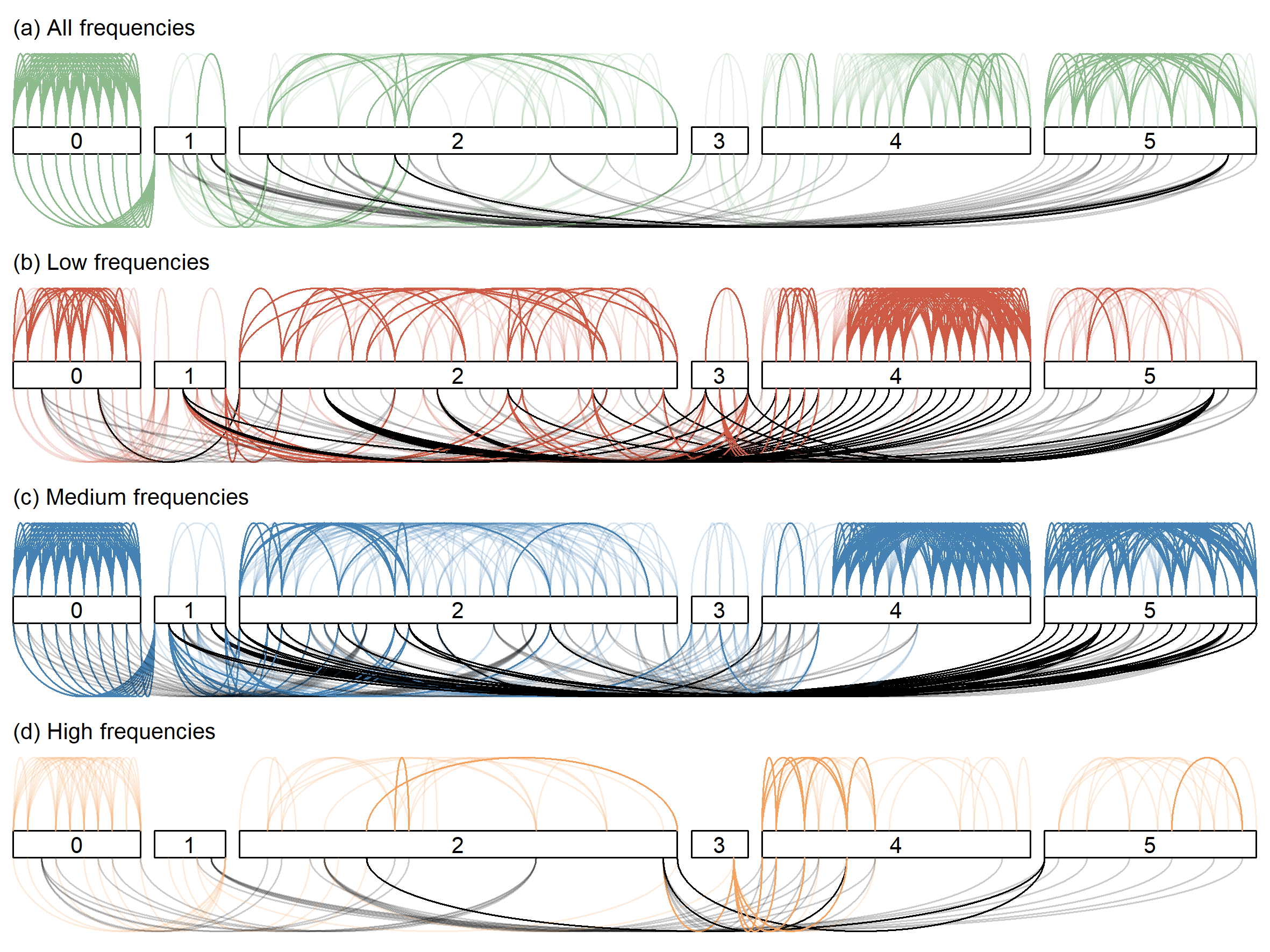
We summarize the results by pairwise coincidence probabilities. The pairwise coincidence probability for subjects and is the probability that they are clustered together. The probabilities are estimated based on 4,000 MCMC samples. Figure 1 summarizes the results. Transparent curves connecting two subjects indicates weak coincidence probability between them in the range and , and a solid curve indicates a probability . The subjects are arranged together if they belong to the same group for easier visualization. Subjects correctly clustered in the same group are linked by curves above the group label. Pairs which are clustered wrongly together but from two similar groups are shown as colored lines below the group labels. Similar groups are ones where the low frequency behaviour is the same, or the high frequency behaviour is the same. Pairs clustered wrongly together with probability from groups that are not similar are shown as black.
We make a number of observations. First, for the low frequency choice of , we never wrongly cluster a strong signal low frequency observation with a weak low frequency observation with high confidence (i.e. no black links below the labels). Similarly, for the high frequency choice of , Figure 1 (d) shows there are no cases of a strong high frequency observation wrongly clustered with weak high frequency observation (again, no black links below the labels). In Figure 1 (d) the classes are ordered differently in the plot for clarity. For the intermediate frequency case, there are few large pairwise coincidence probabilities at all, showing the loss of information about the true groups that occurs when we exclude both high and low frequency basis terms from . When we use all frequencies, the black links below the graph show some cases of individuals clustered together from groups which are not similar. This shows that the filtering of the noise done by integrating out some of the random effects helps for the targeted goal of distinguishing strong/weak low frequency or strong/weak high frequency. This example shows how the choice of can allow the analyst to successfully focus the clustering method on features of the variability of interest for forming clusters.
4.3 Real Example results
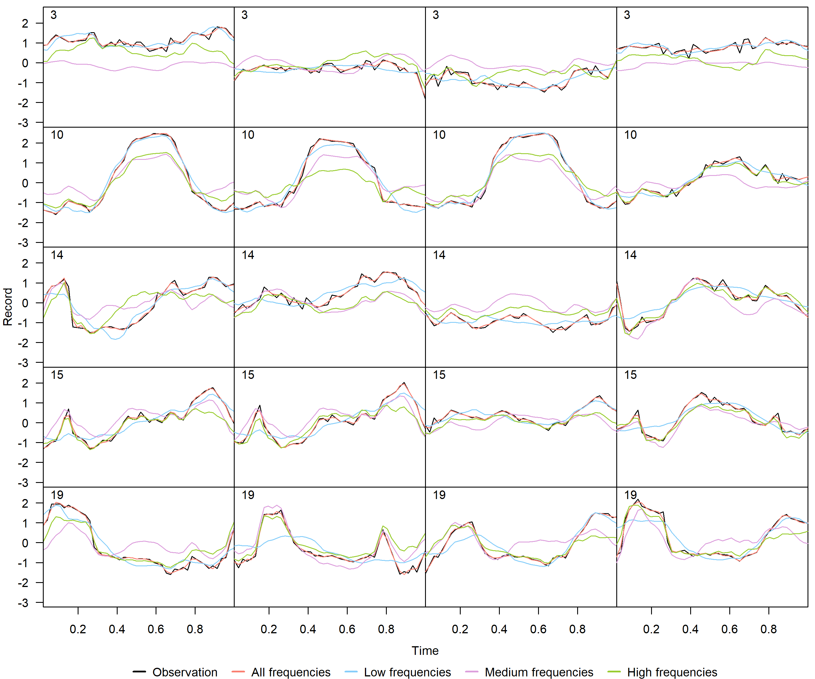
We consider the four real examples next, starting with Example 2. Here and . After fitting the mixed model, Figure 3 shows the fitted means for the mixed predictive replicates in four cases: 1) , 2) (low frequency case), 3) (intermediate frequency case) and 4) (high frequency case). The number plotted in the top left of each figure is the true class label; there are five different values for this label since we randomly sampled 5 of the classes from the original dataset. Four randomly chosen observations for each class are chosen for plotting.
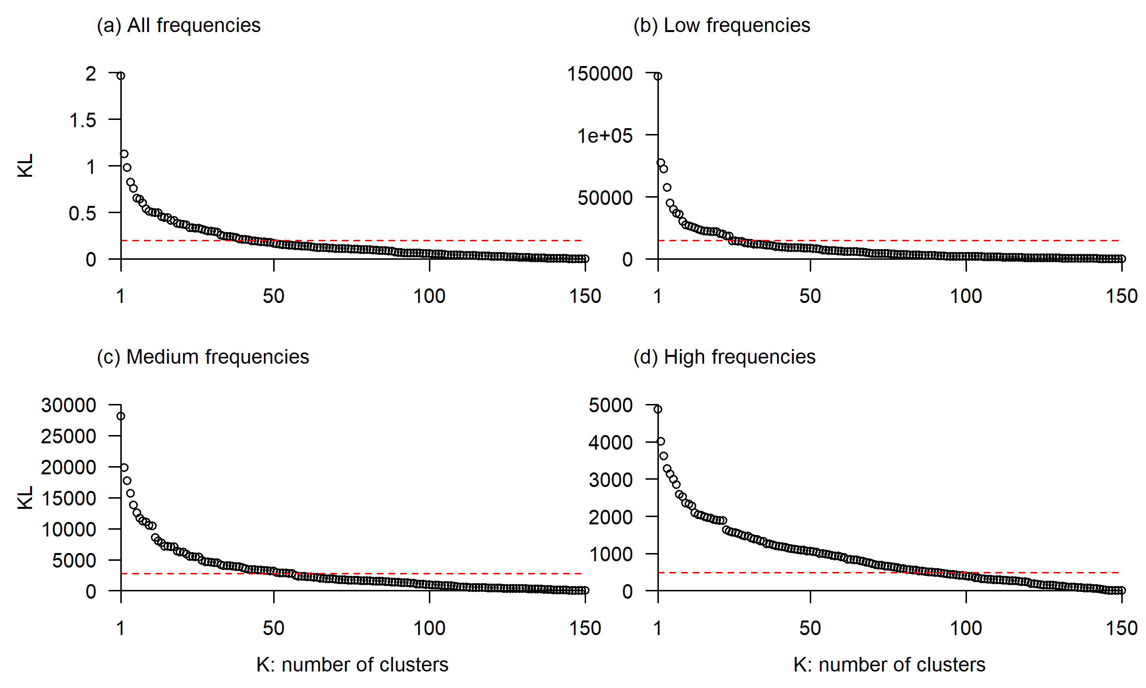
For each choice of , Figure 3 shows a plot of for the bootstrap method against , and the choice of as small as possible subject to being no less than 50% of its maximum value. This results in clusters chosen for the case of all frequencies for , clusters for the low frequency terms for , clusters for the intermedicate frequency for and clusters for high frequency terms for . Using the KL-divergence loss method of choosing the number of clusters described in Section 3 with , gives a large number of clusters for each case (Figure 11 in the Appendix).
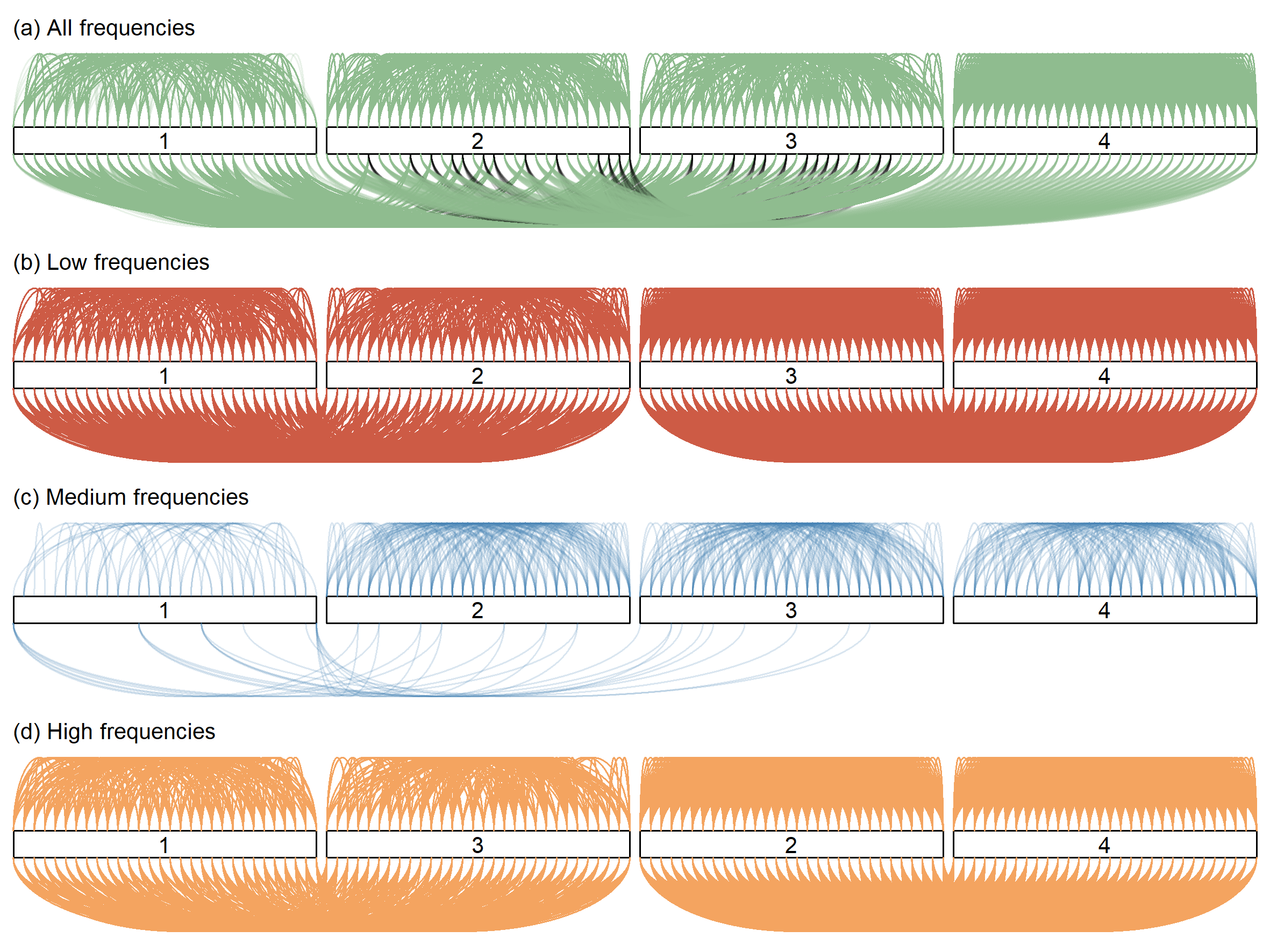
Pairwise coincidence probabilities for our clustering method are shown in Figure 4, where the interpretation of this plot is similar to before for the synthetic data. For clarity we plot only a randomly chosen 10% of the links in the graph. Subjects correctly clustered in the same group are linked by curves above the group label, while those wrongly clustered in different groups are drawn below, with black links for wrong classifications for classes that are not similar. We make the following observations. First, Figure 4 can tell us how informative variation at different scales is for distinguishing between the two classes. The low and intermediate frequency cases for result in a slightly better clustering than the high frequency case, and this can be confirmed quantitatively in the next section where we compare our methods with other benchmarks using the Rand index and adjusted Rand index. Second, we can see that for the low frequency choice of classes 3, 14 and 19 are hard to distinguish, but for the intermediate frequency case they are more easily distinguished (fewer black links below the labels for these classes).
Similar pairwise clustering results for Examples 3-5 are included in the Appendix, and for these cases we use the bootstrap method described in Section 3 for choosing the number of clusters. Plots showing the cluster choice via the bootstrap method for different cases are shown in Figures 11-13 in the Appendix. The bootstrap method tends to give a smaller number of clusters than the method based on the loss in KL divergence due to projection, as shown in Figure 11 in the Appendix for the crop data.
For Example 3, we chose , and low, intermediate and high frequency choices of are , and respectively. For this example, most of the pairs with high pairwise coincidence probability are clustered in the same group or similar groups (next or previous cell stage). Only a few curves appear to wrongly cluster subjects into different groups. Among all the choices for , the low frequency case (Figure 14 (b) in the Appendix) results in better clustering in terms of the true class labels. Again, this can be confirmed in the comparisons with other benchmarks in the next Section. This is an example where filtering out the noise by integrating out some of the random effects actually results in a more accurate clustering in terms of the original class labels.


For Example 4, observations contain seconds of EEG data sampled at Hz, so that there are observations per subject. We apply a discrete Fourier transform to reduce dimension to a set of 40 frequencies by taking the power spectrum for frequencies below Hz: , , where for a signal , , where and . Our observation don’t correspond to observations over time in this example, but are frequency spectrum values at different frequencies , .
Here we consider a B-spline basis for fitting the power spectra. Let be a row vector of cubic B-spline basis functions obtained using equally spaced knots evaluated at the th frequency for observation . The basis functions are ordered according to the knot points, so if we write for the th entry of , basis functions with lower index are locally fitting lower frequencies. We write for the row vector obtained from by extracting components to inclusive. Let , and to capture low, intermediate and high frequency behaviour in our clustering method, we set , and respectively. Figure 15 in the Appendix shows that the intermediate frequency choice for is best for clustering groups 0 and 5.
For Example 5, we define , and our low, intermediate and high frequency choices for are , and respectively. In Example 5, the third activity type is most successfully identified with little noise in the low frequency case (see Figure 16 in the Appendix).
4.4 Comparison with other benchmarks
Now that we have examined how our method can reveal structure at different scales through the choice of , we examine clustering accuracy quantitatively in terms of the true class labels by using the Rand Index (Rand 1971) and adjusted Rand Index (Hubert and Arabie 1985) and compare our method to some other benchmarks. For our method, the Rand and adjusted Rand index values reported are the average values obtained over clusterings obtained from different MCMC samples. In each case, we compare our method with the following alternatives: (1) HC_dist: hierarchical clustering based on an integrated periodogram-based method as dissimilarity measure (Montero and Vilar 2014) (2) HC_pred: hierarchical clustering based on a prediction density-based method as dissimilarity measure (Montero and Vilar 2014) (3) BHC: Bayesian model-based hierarchical clustering with accounting for uncertainty using the Dirichlet process (Savage et al. 2009) (4) KML: -means for longitudinal data (Genolini and Falissard 2011) (5) Mclust: finite Gaussian mixture model under Bayesian framework estimated by Estimation-Maximisation (Scrucca et al. 2016) (6) VC: clustering based on Bayesian mixtures of linear mixed models estimated via variational inference (Tan and Nott 2014). The first five benchmarks can be applied with corresponding R packages but they all require equal time sampled data. The last benchmark is flexible about input data and has R code available online.
For our projection clustering method, the case of all frequencies, low frequencies, intermediate frequencies and high frequencies for are denoted as PC1, PC2, PC3 and PC4 respectively. Table 1 compares our method with the other benhcmark methods for Examples 1-3, and Table 2 compares PC1, PC2, PC3 and PC4 against each other and VC for Example 5, where additional covariates and missingness have been added. The other benchmark methods are not applicable in these cases. In Table 1, the methods PC1 and PC2 are competitive with the best benchmark methods. In Table 2, the addition of covariates allows a small increase in accuracy, while the introduction of missingness causes little deterioration in accuracy of the clustering for capturing the true class labels.
| Example | HC_dist | HC_pred | BHC | KML | Mclust | VC | PC1 | PC2 | PC3 | PC4 |
|---|---|---|---|---|---|---|---|---|---|---|
| Rand Index | ||||||||||
| Eg2 | 0.57 | 0.67 | 0.78 | 0.81 | 0.80 | 0.59 | 0.82 | 0.80 | 0.77 | 0.76 |
| Eg3 | 0.64 | 0.66 | 0.69 | 0.65 | 0.64 | 0.70 | 0.68 | 0.69 | 0.66 | 0.66 |
| Eg4 | 0.75 | 0.70 | 0.74 | 0.78 | 0.77 | 0.68 | 0.79 | 0.78 | 0.80 | 0.75 |
| Adjusted Rand Index | ||||||||||
| Eg2 | 0.10 | 0.04 | 0.35 | 0.41 | 0.40 | 0.10 | 0.45 | 0.38 | 0.30 | 0.29 |
| Eg3 | 0.02 | 0.05 | 0.09 | 0.13 | 0.11 | 0.25 | 0.17 | 0.12 | 0.06 | 0.03 |
| Eg4 | 0.31 | 0.13 | 0.24 | 0.34 | 0.34 | 0.04 | 0.34 | 0.31 | 0.36 | 0.23 |
| Example | VC | PC1 | PC2 | PC3 | PC4 |
|---|---|---|---|---|---|
| Rand Index | |||||
| Eg5 | 0.68 | 0.66 | 0.68 | 0.46 | 0.36 |
| Eg5M | 0.68 | 0.65 | 0.68 | 0.57 | 0.46 |
| Eg5G | 0.67 | 0.64 | 0.67 | 0.46 | 0.41 |
| Adjusted Rand Index | |||||
| Eg5 | 0.04 | 0.05 | 0.04 | 0.06 | 0.05 |
| Eg5M | 0.04 | 0.06 | 0.06 | 0.02 | 0.04 |
| Eg5G | 0.05 | 0.04 | 0.06 | 0.06 | 0.04 |
5 Discussion
We have developed a new model-based clustering method based on mixed predictive replicates and predictive projections. The method fits a linear mixed model, and then defines predictive replicates for each observation where a subset of random effects is shared with the original observations with the other random effects drawn from the conditional prior. Considering predictive projections for the mixed predictive distributions of the replicates, we project onto a space where the number of distinct values for the shared random effects is finite, defining different clusterings. The main strength of the method is the way it gives the analyst flexibility to define what information should be used in defining the clustering, through the choice of shared random effects for defining replicates.
There are several ways this work could be extended. We restricted here to fitting a linear mixed model with Gaussian random effects, but non-Gaussian distributions for the random effects are easily considered. Distributions for the random effects such as finite Gaussian mixtures, multivariate or skew normal having a conditionally Gaussian formulation are easy to use with our method where the latent variables in the conditional Gaussian representation can be generated by MCMC. It would also be possible to consider clustering for discrete data based on generalized linear mixed models, although the computation of projections is more difficult in this case. The methods described in Catalina et al. 2020 for projection predictive model selection in generalized linear and additive mixed models could possibly be used here.
Disclosure Statement
All authors declare no financial conflict.
References
- Akhanli and Hennig (2020) Akhanli, S. E. and C. Hennig (2020). Comparing clusterings and numbers of clusters by aggregation of calibrated clustering validity indexes. arXiv: 2002.01822.
- Bar-Joseph et al. (2002) Bar-Joseph, Z., G. Gerber, D. K. Gifford, T. S. Jaakkola, and I. Simon (2002). A new approach to analyzing gene expression time series data. In Proceedings of the Sixth Annual International Conference on Computational Biology, New York, NY, USA, pp. 39–48. Association for Computing Machinery.
- Booth et al. (2008) Booth, J. G., G. Casella, and J. P. Hobert (2008). Clustering using objective functions and stochastic search. Journal of the Royal Statistical Society: Series B (Statistical Methodology) 70(1), 119–139.
- Bouveyron et al. (2019) Bouveyron, C., G. Celeux, T. B. Murphy, and A. Raftery (2019). Model-Based Clustering and Classification for Data Science. Cambridge University Press.
- Bush and MacEachern (1996) Bush, C. A. and S. N. MacEachern (1996). A semiparametric Bayesian model for randomised block designs. Biometrika 83(2), 275–285.
- Casale et al. (2012) Casale, P., O. Pujol, and P. Radeva (2012). Personalization and user verification in wearable systems using biometric walking patterns. Personal and Ubiquitous Computing 16(5), 563–580.
- Catalina et al. (2020) Catalina, A., P.-C. Bürkner, and A. Vehtari (2020). Projection predictive inference for generalized linear and additive multilevel models. arXiv:2010.06994 [stat]. arXiv: 2010.06994.
- Celeux et al. (2005) Celeux, G., O. Martin, and C. Lavergne (2005). Mixture of linear mixed models for clustering gene expression profiles from repeated microarray experiments. Statistical Modelling 5(3), 243–267.
- Coke and Tsao (2010) Coke, G. and M. Tsao (2010). Random effects mixture models for clustering electrical load series. Journal of Time Series Analysis 31(6), 451–464.
- Dau et al. (2019) Dau, H. A., A. Bagnall, K. Kamgar, C.-C. M. Yeh, Y. Zhu, S. Gharghabi, C. A. Ratanamahatana, and E. Keogh (2019). The UCR Time Series Archive. arXiv: 1810.07758.
- De la Cruz-Mesía et al. (2008) De la Cruz-Mesía, R., F. A. Quintana, and G. Marshall (2008). Model-based clustering for longitudinal data. Computational Statistics and Data Analysis 52(3), 1441–1457.
- DeYoreo et al. (2017) DeYoreo, M., J. P. Reiter, and D. S. Hillygus (2017). Bayesian mixture models with focused clustering for mixed ordinal and nominal data. Bayesian Analysis 12(3), 679–703.
- Dua and Graff (2017) Dua, D. and C. Graff (2017). UCI machine learning repository. http://archive.ics.uci.edu/ml.
- Dupuis and Robert (2003) Dupuis, J. A. and C. P. Robert (2003). Variable selection in qualitative models via an entropic explanatory power. Journal of Statistical Planning and Inference 111(1), 77–94.
- Fang and Wang (2012) Fang, Y. and J. Wang (2012). Selection of the number of clusters via the bootstrap method. Computational Statistics & Data Analysis 56(3), 468–477.
- Gelman et al. (1996) Gelman, A., X.-L. Meng, and H. Stern (1996). Posterior predictive assessment of model fitness via realized discrepancies. Statistica Sinica 6, 733–807.
- Genolini and Falissard (2011) Genolini, C. and B. Falissard (2011). Kml: A package to cluster longitudinal data. Computer Methods and Programs in Biomedicine 104(3), e112–e121.
- Heard et al. (2006) Heard, N. A., C. C. Holmes, and D. A. Stephens (2006). A quantitative study of gene regulation involved in the immune response of anopheline mosquitoes. Journal of the American Statistical Association 101(473), 18–29.
- Heinzl and Tutz (2013) Heinzl, F. and G. Tutz (2013). Clustering in linear mixed models with approximate Dirichlet process mixtures using EM algorithm. Statistical Modelling 13(1), 41–67.
- Hubert and Arabie (1985) Hubert, L. and P. Arabie (1985). Comparing partitions. Journal of Classification 2, 193–218.
- Jacques and Preda (2014) Jacques, J. and C. Preda (2014). Functional data clustering: a survey. Advances in Data Analysis and Classification 8(3), 231–255.
- James and Sugar (2003) James, G. M. and C. A. Sugar (2003). Clustering for sparsely sampled functional data. Journal of the American Statistical Association 98(462), 397–408.
- Kleinman and Ibrahim (1998) Kleinman, K. P. and J. G. Ibrahim (1998). A semiparametric Bayesian approach to the random effects model. Biometrics 54(3), 921–938.
- Luan and Li (2003) Luan, Y. and H. Li (2003). Clustering of time-course gene expression data using a mixed-effects model with B-splines. Bioinformatics 19(4), 474–482.
- McDowell et al. (2018) McDowell, I. C., D. Manandhar, C. M. Vockley, A. K. Schmid, T. E. Reddy, and B. E. Engelhardt (2018). Clustering gene expression time series data using an infinite Gaussian process mixture model. PLoS Computational Biology 14(1).
- McLachlan and Peel (2000) McLachlan, G. J. and D. Peel (2000). Finite mixture models. New York: Wiley Series in Probability and Statistics.
- Montero and Vilar (2014) Montero, P. and J. A. Vilar (2014). TSclust: An R Package for Time Series Clustering. Journal of Statistical Software 62(1), 1–43.
- Müller and Rosner (1997) Müller, P. and G. L. Rosner (1997). A Bayesian population model with hierarchical mixture priors applied to blood count data. Journal of the American Statistical Association 92(440), 1279–1292.
- Ng et al. (2006) Ng, S. K., G. J. McLachlan, K. Wang, L. Ben-Tovim Jones, and S.-W. Ng (2006). A Mixture model with random-effects components for clustering correlated gene-expression profiles. Bioinformatics 22(14), 1745–1752.
- Pauler and Laird (2000) Pauler, D. K. and N. M. Laird (2000). A mixture model for longitudinal data with application to assessment of noncompliance. Biometrics 56(2), 464–472.
- Pfeifer (2004) Pfeifer, C. (2004). Classification of longitudinal profiles based on semi-parametric regression with mixed effects. Statistical Modelling 4(4), 314–323.
- Piironen et al. (2020) Piironen, J., M. Paasiniemi, and A. Vehtari (2020). Projective inference in high-dimensional problems: Prediction and feature selection. Electronic Journal of Statistics 14(1), 2155 – 2197.
- Rand (1971) Rand, W. M. (1971). Objective criteria for the evaluation of clustering methods. Journal of the American Statistical Association 66(336), 846–850.
- Ray and Mallick (2006) Ray, S. and B. Mallick (2006). Functional clustering by Bayesian wavelet methods. Journal of the Royal Statistical Society: Series B (Statistical Methodology) 68(2), 305–332.
- Rigon and Dunson (2020) Rigon, Tommaso, H. A. H. and D. B. Dunson (2020). A generalized Bayes framework for probabilistic clustering. arXiv:2006.05451.
- Savage et al. (2009) Savage, R. S., K. Heller, Y. Xu, Z. Ghahramani, W. M. Truman, M. Grant, K. J. Denby, and D. L. Wild (2009). R/BHC: fast Bayesian hierarchical clustering for microarray data. BMC Bioinformatics 10(1), 242.
- Scharl et al. (2010) Scharl, T., B. Grün, and F. Leisch (2010). Mixtures of regression models for time course gene expression data: evaluation of initialization and random effects. Bioinformatics 26(3), 370–377.
- Scrucca et al. (2016) Scrucca, L., M. Fop, T. Murphy, Brendan, and A. Raftery, E. (2016). mclust 5: Clustering, classification and density estimation using Gaussian finite mixture models. The R Journal 8(1), 289.
- Shi and Wang (2008) Shi, J. Q. and B. Wang (2008). Curve prediction and clustering with mixtures of Gaussian process functional regression models. 18(3), 267–283.
- Spellman et al. (1998) Spellman, P. T., G. Sherlock, M. Q. Zhang, V. R. Iyer, K. Anders, M. B. Eisen, P. O. Brown, D. Botstein, and B. Futcher (1998). Comprehensive Identification of Cell Cycle–regulated Genes of the Yeast Saccharomyces cerevisiae by Microarray Hybridization. Molecular Biology of the Cell 9(12), 3273–3297.
- Stan Development Team (2021) Stan Development Team (2021). Stan modeling language users guide and reference manual, 2.21.2.
- Tan and Nott (2014) Tan, S. L. and D. J. Nott (2014). Variational approximation for mixtures of linear mixed models. Journal of Computational and Graphical Statistics 23(2), 564–585.
- Terzano et al. (2001) Terzano, M. G., L. Parrino, A. Sherieri, R. Chervin, S. Chokroverty, C. Guilleminault, M. Hirshkowitz, M. Mahowald, H. Moldofsky, A. Rosa, R. Thomas, and A. Walters (2001). Atlas, rules, and recording techniques for the scoring of cyclic alternating pattern (CAP) in human sleep. Sleep Medicine 2(6), 537–553.
Appendix - Additional Figures