Two-Stage TMLE to Reduce Bias and Improve Efficiency
in Cluster Randomized Trials
Cluster randomized trials (CRTs) randomly assign an intervention to groups of individuals (e.g., clinics or communities) and measure outcomes on individuals in those groups. While offering many advantages, this experimental design introduces challenges that are only partially addressed by existing analytic approaches. First, outcomes are often missing for some individuals within clusters. Failing to appropriately adjust for differential outcome measurement can result in biased estimates and inference. Second, CRTs often randomize limited numbers of clusters, resulting in chance imbalances on baseline outcome predictors between arms. Failing to adaptively adjust for these imbalances and other predictive covariates can result in efficiency losses. To address these methodological gaps, we propose and evaluate a novel two-stage targeted minimum loss-based estimator (TMLE) to adjust for baseline covariates in a manner that optimizes precision, after controlling for baseline and post-baseline causes of missing outcomes. Finite sample simulations illustrate that our approach can nearly eliminate bias due to differential outcome measurement, while existing CRT estimators yield misleading results and inferences. Application to real data from the SEARCH community randomized trial demonstrates the gains in efficiency afforded through adaptive adjustment for baseline covariates, after controlling for missingness on individual-level outcomes.
Key words: Clustered data; Cluster randomized trials; Covariate adjustment; Data-adaptive; Double robust; Group randomized trials; Missing data; Multi-level model; Super Learner; TMLE.
1 Introduction
In many trials, treatments are randomly allocated to groups of individuals, such as hospitals, schools, or communities, and outcomes are measured on individuals in those groups. These studies are known as group or cluster randomized trials (CRTs). They are implemented when the treatment is naturally delivered to the group or when substantial dependence between individuals within groups is expected [1, 2, 3, 4, 5]. CRTs are rapidly increasing in popularity; a recent review found a 280-fold increase in their use from 1995 to 2015 [6]. Nonetheless, despite extensive research dedicated to their design and conduct, this review also concluded only half of CRTs were analyzed appropriately. CRTs can provide gold-standard evidence of causality, but they face several methodological challenges.
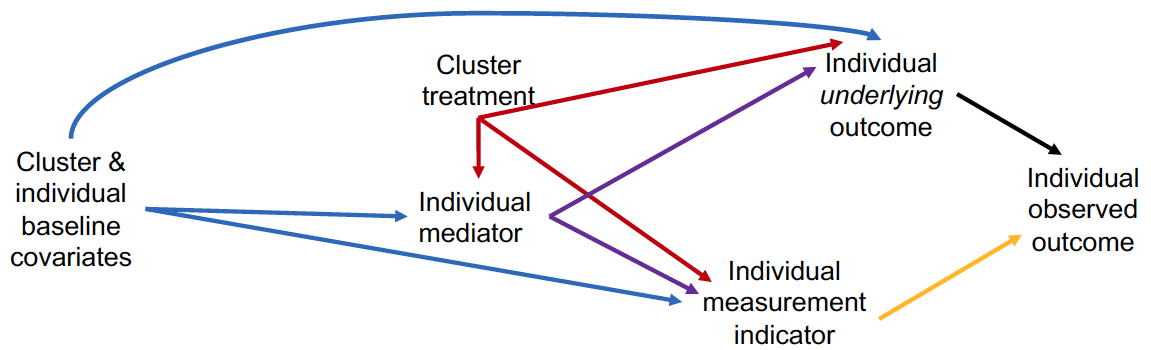
First, missing participant outcomes occur in over 90% of CRTs [7]. When participants with missing outcomes differ meaningfully from those with measured outcomes, complete-case analyses yield biased estimates [8, 9]. This potential for bias is exacerbated when, as commonly occurs, the cluster randomized intervention, itself, influences outcome measurement. Suppose, for example, that the cluster-level intervention increases care engagement, which in turn improves both participants’ outcomes and their chances of having that outcome measured (Figure 3 in Supplementary Materials). Here, an unadjusted comparison of outcomes between arms can overestimate or underestimate the treatment effect. Even if key determinants of missingness, such as care engagement, are measured, standard analytic approaches to CRTs will fail to control for this bias, because care engagement simultaneously mediates the treatment-outcome relationship and confounds the missingness-outcome relationship [10, 9, 11].
Second, CRTs often randomize limited numbers of groups; a review found a median of 33 clusters randomized [12]. Even when some form of restricted randomization (e.g., pair-matching) is used, CRTs with few clusters are likely to suffer from chance imbalances between treatment arms on baseline determinants of the outcome. Adjustment for these covariates and others predictive of the outcome (hereafter called “covariate imbalance”) can increase statistical power (e.g., [13, 14, 15, 1, 16, 4, 6, 5]). The adjustment approach is often with an outcome regression, characterizing the expected outcome given the treatment assignment and covariates. This regression must be a priori-specified to avoid inflating Type-I error rates. Additionally to avoid over-fitting, a limited number of adjustment variables must be selected from a typically large set of candidates, risking forced adjustment for variables that prove useless for, or even detrimental to, precision [17, 18, 19]. Thus, we wish to define a fully pre-specified procedure for CRT analysis that optimizes statistical power through data-adaptive adjustment of baseline covariates, while rigorously preserving Type-I error control.
In this manuscript, we propose and evaluate a novel estimator that addresses the dual challenges of bias due to missing outcomes and imprecision due to few randomized units in CRTs. Our approach uses targeted minimum loss-based estimation (TMLE; [15]) in two stages: first at the individual-level to adjust for differential measurement of individual-level outcomes and second at the cluster-level to improve efficiency when estimating the intervention effect. Therefore, we refer to our estimator as “Two-Stage TMLE”. To the best of our knowledge, Two-Stage TMLE is the first semiparametric efficient estimator that adaptively adjusts for both individual-level missingness and for covariate imbalance in CRTs. It can be applied to estimate a range of causal parameters and under a range of CRT study designs, including differing randomization schemes (e.g., pair-matched or not) and approaches to participant follow-up within clusters (e.g., cross-sectional sampling or longitudinal follow-up).
2 Brief Review of CRT Methods
We provide an overview of existing CRT methods in Table 1 and refer the reader to [20] for a detailed review. A simple two-stage approach to account for the dependence of participants within clusters is to aggregate the individual-level data to the cluster-level and then implement an effect estimator appropriate for independent data, such as a -test. Use of an unadjusted effect estimator in the second stage avoids modeling assumptions and the risk of over-fitting, but by ignoring covariate information is inefficient (e.g., [13, 14, 15, 1, 16, 4, 6, 5]).
In contrast, mixed models and generalized estimating equations (GEE) typically adjust for a number of baseline individual- and cluster-level covariates, providing an opportunity to improve precision of effect estimates [21, 22]. However, neither address the need for a pre-specified approach to select the adjustment variables that optimize efficiency, while preserving valid statistical inference. Further, both are susceptible to allowing the estimator choice define the effect measure that is estimated (e.g., GEE with a logistic link yields estimates of the conditional odds ratio) [23].
To the best of our knowledge, only three methods generally allow for estimation of marginal effects in CRTs, while adjusting for individual- and cluster-level covariates. First, in the covariate adjusted residuals estimator (CARE), cluster-level outcomes are compared with those predicted from an individual-level regression of the outcome on individual- and cluster-level covariates, but not the cluster-level treatment [14, 1]. Second, augmented-GEE extends GEE for the marginal effect by including an “augmentation” term, inspired by the efficient influence function [24, 17, 25]. Finally, hierarchical TMLE extends TMLE for estimation of marginal effects with cluster-based exposures ([26, 20]; overview in the Supplementary Materials).
With regards to missingness, an unadjusted effect estimator requires the strongest identification assumption: there are no common causes of missingness and outcomes (i.e., the missing-completely-at-random, or MCAR, assumption holds) [8]. The other methods rely on a weaker identification assumption; essentially, that the outcome distributions among persons for which the outcome is measured versus missing are exchangeable conditional on the treatment arm and some subset of measured covariates [4, 27, 28].
Combining Augmented-GEE with inverse probability weighting yields a double robust estimator (“DR-GEE”); it is nearly unbiased if either the outcome regression or the measurement mechanism (i.e., the conditional probability of outcome measurement given the treatment arm and covariates) is correctly specified [29]. To the best of our knowledge, DR-GEE’s methodology and computing code have been limited to adjustment for baseline variables only. Hierarchical TMLE also offers the potential for integrated precision gains and double robust adjustment. However, these extensions remain to be fully studied. Here, we, instead, develop and evaluate Two-Stage TMLE to (1) control for potentially differential missingness in each cluster separately, and (2) adaptively adjust for covariate imbalance to improve efficiency when estimating the intervention effect. Before doing so, we present our motivating example.
3 Motivating Example
The SEARCH Study was a pair-matched, pragmatic CRT of 32 communities each with 10,000 persons in rural Kenya and Uganda (ClinicalTrials.gov: NCT01864603) [30]. SEARCH was designed to evaluate the population-level effects of annual multi-disease testing and universal treatment for persons with HIV (intervention) versus baseline multi-disease testing and country-guided treatment (active control) on a range of outcomes including incident HIV, viral suppression among persons with HIV, hypertension control, and incident tuberculosis (TB).
As with the vast majority of CRTs, outcomes were not measured among all SEARCH participants and the MCAR assumption was unreasonable for many endpoints. Additionally, despite matching prior to randomization [31], covariate imbalance was expected; however, it was unclear a priori which covariates to include in the adjustment set for optimal gains in efficiency. To reduce bias from missingness on individual-level outcomes and to maximize precision during effect estimation in the SEARCH Study, we developed Two-Stage TMLE.
4 Two-Stage TMLE
In many CRTs, outcomes are assessed through longitudinal follow-up of a closed cohort of participants. In the SEARCH Study, for example, the primary outcome was the three-year cumulative incidence of HIV: the proportion of community residents ( 15 years) who were HIV-uninfected at baseline and became infected with HIV over the three-year study. To assess the treatment effect on such endpoints, a cohort of participants who are at risk of the outcome is defined in each cluster. For each participant, let denote their baseline covariates, be their post-intervention covariates, be an indicator of outcome measurement, and be the outcome of interest. The outcome is only observed when . We also observe cluster-level covariates and the randomly assigned cluster-level intervention . Throughout, superscript will be used to distinguish cluster-level variables from individual-level variables. We denote the observed data structure for a participant as . In the SEARCH Study, for example, included baseline HIV prevalence and male circumcision coverage; included age, sex, marital status, occupation, education, and mobility; was a community-level indicator of randomization to the intervention; was interim HIV testing; was an indicator of HIV testing at year 3, and was an indicator of having a confirmed HIV-positive diagnosis at year 3 testing.
Recall our goal is to simultaneously control for differential missingness on individual-level outcomes, while estimating the effect of the cluster-level intervention with optimal precision. To do so, we consider an individual-level counterfactual outcome , generated by hypothetical interventions on the cluster-level treatment (i.e., to “set” ) and the measurement mechanism (i.e., to “set” ). Identification of a corresponding causal parameter (e.g., ) is complicated by clustering and the missing data equivalent to time-dependent confounding (Figure 1). Instead, in our novel Two-Stage approach, we separate control for missing outcomes (Stage 1) from evaluation of the intervention effect (Stage 2). Specifically, in Stage 1, we fully stratify on each cluster, vastly simplifying identifiability and estimation for the missing data problem (Figure 2). Then in Stage 2, we use the estimates from Stage 1 to evaluate the intervention effect. Our approach allows the missingness mechanism to vary by cluster, while avoiding specifying complex relationships between individual-level (, ) and cluster-level variables (.
4.1 Stage 1: Identifying and Estimating Cluster-Specific Endpoints
For the purposes of controlling for differential outcome measurement, we consider each of the clusters separately in Stage 1. Since the cluster-level covariates and treatment are constant within each cluster, the Stage 1 observed data simplify to and the target causal parameter to . Then if MCAR held in each cluster or, equivalently, , this causal parameter could be identified as and consistently estimated as the empirical mean among those measured within each cluster: . We relax this missing data assumption by allowing measurement to depend on the participant’s baseline and time-varying characteristics . Specifically, if and there is sufficient data support (i.e., the positivity assumption holds), our Stage 1 statistical estimand would be
| (1) |
Within each cluster separately, could be estimated by a variety of algorithms, including inverse-weighting and G-computation [32, 10]. We use TMLE for estimation the cluster-specific endpoint , given its asymptotic properties and improved finite sample performance (e.g., [15, 33]). Briefly, TMLE combines estimates of the outcome regression with those of the measurement mechanism . In doing so, TMLE achieves a number of desirable properties, including double robustness: a consistent estimate is attained if either the outcome regression or the measurement mechanism is consistently estimated. If both are consistently estimated at reasonable rates, TMLE will be efficient. In practice, we recommend implementing TMLE using Super Learner, an ensemble machine learning algorithm [34]. Step-by-step implementation for Eq. 2 is given in the Supplementary Materials. Since we are fully stratifying on cluster, an individual-level TMLE would be implemented times to obtain cluster-specific estimates: , where indexes the participants in a given cluster and denotes the targeted prediction of the individual-level outcome for participant in that cluster.
4.1.1 Stage 1 with Survival-Type Endpoints:
When assessing effects on time-to-event outcomes, participants are followed longitudinally until the occurrence of the event of interest or right-censoring. Examples of such endpoints in the SEARCH Study included the probability of treatment initiation and the cumulative risk of HIV-associated TB or death due to illness. Our framework also accommodates survival-type endpoints. Specifically, to account for right-censoring in Stage 1, we would identify a different cluster-specific endpoint and estimate it using the Kaplan-Meier estimator when censoring is non-differential or TMLE when censoring is differential [35, 36].
4.1.2 Stage 1 with Endpoints Measured in a Cross-Sectional Design:
Other endpoints may be assessed using a cross-sectional design, where participants are measured at a single timepoint. In these settings, we may have missingness on the characteristic defining the sub-population of interest as well as the outcome of interest. Consider, for example, population-level HIV viral suppression, defined as the proportion of all HIV-infected persons whose plasma HIV RNA level is suppressed below some limit: . Both baseline and time-varying factors impact HIV status and its measurement as well as viral suppression and its measurement. To handle missingness on both the outcome (viral suppression) and the conditioning set (HIV-positivity), we redefine the outcome as the joint probability of being HIV-infected and suppressing viral replication, divided by HIV prevalence: . Again our Two-Stage approach can accommodate this ratio-type endpoint. Specifically, we would identify estimate (with TMLE) the numerator and denominator separately, and then take their ratio to estimate a new cluster-specific endpoint in Stage 1 [37].
4.2 Stage 2: Estimation of the Effect of the Cluster-level Intervention
Recall in Stage 1, we stratify on each cluster to identify and estimate a cluster-specific endpoint that accounts for potentially differential measurement or censoring at the individual-level (e.g., Eq. 2). Then in Stage 2, our goal is to use those estimates to evaluate the intervention effect with maximum precision. The Supplementary Materials provide a detailed discussion of several Stage 2 causal effects, which are all easily identified due to randomization of the cluster-level treatment and prior control for missingess in Stage 1. For estimation of these effects in Stage 2, the observed data can be simplified to the cluster-level: , where represents the baseline cluster-level covariates; denotes summary measures of the baseline individual-level covariates; is an indicator of randomization to the intervention arm, and is the estimated cluster-specific endpoint from Stage 1.
With these data, a simple estimator of the treatment effect is the average outcome among intervention clusters contrasted with the average outcome among control clusters . Instead, to obtain a more efficient estimate of the intervention effect (e.g., [38, 39]), we implement a cluster-level TMLE in Stage 2. Briefly, an initial estimator of the cluster-level outcome regression is updated based on an estimate of the cluster-level propensity score to achieve a targeted estimator . Targeted estimates of the expected outcomes under the intervention and under the control are generated for all clusters, averaged across clusters, and contrasted. Step-by-step implementation of TMLE in Stage 2 is given in the Supplementary Materials.
Unfortunately, it is nearly impossible to a priori-specify the optimal estimators of the outcome regression and propensity score . Few clusters prohibit the use of Super Learner. To avoid over-fitting while flexibly selecting the adjustment variables that maximize precision, we recommend using Adaptive Pre-specification in Stage 2 [18]. The procedure data-adaptively selects from a pre-specified set the candidate adjustment variables and, thus, the TMLE that maximize empirical efficiency. Briefly, we pre-specify (1) candidate adjustment variables that are predictive of the outcome, (2) a loss function corresponding to the squared influence curve for the TMLE of the target effect, and (3) a sample-splitting scheme; leave-one-out cross-validation is recommended. The candidate adjustment variables then define the set of candidate estimators for the outcome regression and the propensity score based on “working” generalized linear models (GLMs). The procedure data-adaptively choses the combination of the outcome regression and propensity score GLMs (and thus the TMLE) with the lowest cross-validated variance estimate. Adaptive Pre-specification is an extension of Collaborative-TMLE using a cross-validation selector to maximize precision in small trials.
In CRTs with few clusters, we recommend limiting the candidate GLMs to a single adjustment covariate. In CRTs with many clusters, we could also include candidate GLMs adjusting for multiple covariates and allow the procedure to data-adaptively determine the size of the adjustment set. Simulations mimicking the real data application (e.g., in sample size and expected within cluster dependence) can help inform these choices. Importantly, there is no guarantee that adjusting for more covariates will improve empirical efficiency. For some CRTs, none of the pre-specified covariates will improve precision over the unadjusted estimator. In this setting, the procedure will select the unadjusted effect estimator. Altogether with Adaptive Pre-specification, decisions about whether and how to adjust for optimal precision gains in Stage 2 are made with a rigorous procedure that does not compromise Type-I error.
4.3 Statistical Inference for Two-Stage TMLE
Now we have a point estimate of the intervention effect and are ready to obtain statistical inference, which occurs at the cluster-level. Under the following conditions, detailed in the Supplementary Materials, Two-Stage TMLE is an asymptotically linear estimator of the intervention effect , meaning that , where is the cluster-level influence curve and is the remainder term, going to zero in probability [40]:
- 1.
Stage 1 estimation of the cluster-level outcomes provides negligible contribution to ;
- 2.
Stage 2 estimators of the cluster-level outcome regression and the cluster-level propensity score satisfy the usual regularity conditions (e.g., [38]).
The second condition is automatically satisfied when Adaptive Pre-specification is used to select among GLMs for the outcome regression and the known propensity score . However, to satisfy the first condition we need (i) the Stage 1 estimators of the individual-level outcome regression and the individual-level measurement mechanism to converge to their targets at fast enough rates, (ii) the within cluster dependence to be weak enough that the Central Limit Theorem applies in cluster size , and (iii) the cluster size is large relative to the total number of clusters (i.e., ; Supplementary Materials).
While these are asymptotic requirements, the Stage 1 conditions highlight the importance of having sufficiently sized clusters to support our missing data assumptions and to allow for flexible estimation of the individual-level outcome regression and measurement mechanism in Stage 1. Small cluster sizes may force us to rely on strong identifiability assumptions (e.g., MCAR within each cluster or only dependent on a single covariate) and strong estimation assumptions (e.g., the probability of being measured is accurately described by a main terms logistic regression). Such assumptions may or may not be reasonable in a given application. Larger cluster sizes, however, permit the use TMLE with Super Learner to flexibly adjust for the baseline and time-dependent covariates influencing outcomes and measurement in each cluster in Stage 1. TMLE is also double robust, providing a consistent estimate of the cluster-specific endpoint if either the individual-level outcome regression or measurement mechanism is consistently estimated. Altogether, the requirements for valid statistical inference are not unique to our proposed approach; they apply to other two-stage estimators (e.g., a -test on the mean outcome among those measured). In all cases, if the cluster-level endpoints are estimated poorly in Stage 1, we are risk of biased point estimates and misleading conclusions in Stage 2. Simulations, below, explore the finite sample performance of Two-Stage TMLE under challenges commonly faced by CRTs: few clusters of modest size, correlated outcomes within clusters, and differential outcome measurement.
When the above conditions hold, the limit distribution of the standardized estimator is normal with mean 0 and variance given by the variance of its influence curve. For the treatment-specific mean , for example, the influence curve for Two-Stage TMLE is approximated as . We obtain a variance estimate with the sample variance of the estimated influence curve divided by the number of independent units . Then using the Student’s -distribution with degrees of freedom as a finite sample approximation to the normal distribution [1], we can construct Wald-Type 95% confidence intervals and conduct hypothesis testing. Additionally, through the Delta Method, we can derive the influence curve and variance estimator for the intervention effect on any scale of interest. For the absolute effect , the estimated influence curve for TMLE would be . For the relative effect , we would apply the Delta method on the log-scale [38]. This approach to statistical inference also applies when the treatment is randomized within matched pairs of clusters (Supplementary Materials).
5 Simulation Study
We examine the finite sample performance of our proposed estimator using simulations to incorporate common CRT challenges, such as few randomized clusters and differential missingness. Specifically, we focus on a setting with clusters and where within each cluster, the number of individual participants is sampled with equal probability from {100, 150, 200}. In these simulations, both baseline and post-baseline covariates impact measurement of individual-level outcomes. Additional simulations and computing code are given in the Supplementary Materials.
5.1 Data Generating Process
For each cluster , we independently generate the cluster-specific data as follows. First, three cluster-level, latent variables are independently generated as , , and . Then, two individual-level covariates are drawn independently from normal distributions with cluster-specific means: and . We set the observed cluster-level covariates as the empirical mean of their individual-level counterparts. The cluster-level intervention is randomly allocated within pairs of clusters matched on .
The individual-level mediator is generated as an indicator that is less than the . The underlying, individual-level outcome is generated as an indicator that is less than . Finally, individual-level measurement is generated as an indicator that is less than . Thus, the measurement mechanism is highly differential by treatment arm with a mean of 70% measured in the intervention arm and 43% in the control arm. The observed outcomes are set to missing for individuals with .
We also generate the counterfactual mediators and outcomes by setting the cluster-level treatment and preventing missingness (i.e., setting ). The cluster-level, counterfactual outcome is the average of the individual-level, counterfactual outcomes within each cluster. We generate a population of 5000 clusters and calculate the true value of the treatment-specific, population means for , their difference, and their ratio.
5.2 Estimators Compared in the Simulation Study
We compare a variety of estimators commonly implemented in CRTs. We consider 4 complete-case approaches, in which the data are subset to exclude participants with missing outcomes (i.e., those with ): an unadjusted estimator, CARE, mixed models, and GEE. We also implement 2 approaches which use data on all participants: DR-GEE and our Two-Stage TMLE.
For the unadjusted approach, we first aggregate the individual-level outcomes to the cluster-level by taking the empirical mean among those measured (i.e., ) and then contrast the average cluster-level outcomes by treatment arm with inference from the -distribution. For CARE, we pool data across clusters and run logistic regression of the individual-level outcome on the baseline covariates ; calculate the residuals by taking the difference between the cluster-level outcomes (the empirical mean among those measured) and those predicted from the previous regression, and finally use a -test to compare the residuals by arm.
In mixed models and GEE, we again pool data across clusters and fit a log-linear regression of the individual-level outcome on the cluster-level treatment and baseline covariates .
In DR-GEE, we also estimate the measurement mechanism with a pooled logistic regression of on
and the augmentation terms with arm-specific log-linear regressions of on
.
To account for within cluster dependence, we include a random cluster-specific intercept in mixed models and use an independent working correlation matrix in the GEEs.
For mixed models, GEE, and DR-GEE, the default settings of lme4, geepack, and CRTgeeDR packages are used for standard error estimation, respectively.
For Two-Stage TMLE, we first implement an individual-level TMLE within each cluster separately to estimate the cluster-specific endpoint . In these TMLEs, the outcome regression and the measurement mechanism are estimated using Super Learner to combine predictions from main terms logistic regression, generalized additive models, and the empirical mean. In Stage 2, we compare these cluster-specific estimates by treatment arm using a cluster-level TMLE with Adaptive Pre-specification to select the optimal adjustment variables from and with inference via the estimated influence curve (Section 4.3).
5.3 Simulation Results
The average coefficient of variation was 0.24 in the intervention arm and 0.17 in the control arm, reflecting expected levels of dependence between individual-level outcomes within clusters [1]. The true values of the risk difference and risk ratio were -9.1% and 0.88, respectively. For both effects, Table 2 summarizes estimator performance when “breaking the matches” (i.e., ignoring the pair-matching scheme used for treatment randomization) and when preserving the matches. The exception is for DR-GEE, because to our knowledge, there does not yet exist an extension of DR-GEE for pair-matched CRTs.
Focusing first on estimators of the risk difference (true value=-9.1%), we see that -test, which does not adjust for covariates, is highly biased, as expected given the differential measurement process. On average, it grossly overestimates the effect by 22.9% and attains confidence interval coverage of 1%. By adjusting for covariates, CARE is less biased, but still overestimates the intervention effect by 12.7% when breaking the matches and by 9.9% when preserving the matches. The corresponding confidence interval coverages are much less than the nominal rate: 7.8% and 40.4%, respectively. In contrast, the bias of Two-Stage TMLE is low (1%) and confidence interval coverage is good (95%). Also as predicted by theory [31], more power is achieved when preserving (57.4%) versus breaking the matches (52.8%).
Now focusing on estimators of the risk ratio (true value=0.88), both mixed models and GEE overestimate the effect, preventing accurate inference. The confidence interval coverage is 5.6-7.0% for mixed models and 1.2-4.8% for GEE. These estimators are expected to be unbiased when there are only baseline causes of missingness and the outcome regressions are correctly specified. Here, there are post-baseline causes of missingness, which are simultaneously mediators of the treatment-outcome relationship. DR-GEE is expected to reduce bias due to missing outcomes by incorporating weights corresponding to the measurement mechanism, and this is seen when there are only baseline causes of missingness (Table 1 in Supplementary Materials). However, extensions of DR-GEE to handle post-baseline causes of missingness do not yet exist, and in the main simulations, DR-GEE attains 1% confidence interval coverage for the risk ratio (Table 2).
In contrast, Two-Stage TMLE is essentially unbiased and achieves good confidence interval coverage (95%) for the risk ratio. Again, more power is achieved when keeping (57.8%) versus breaking the matches (52.6%). In further simulation studies given in the Supplementary Materials, Two-Stage TMLE also performs well with fewer clusters and maintains nominal Type-I error control when there is no effect. Finally, as shown in the Supplementary Materials, including the mediator in the adjustment set of the existing methods does not improve their performance.
6 Application to the SEARCH Study
The results of the SEARCH Study have been previously published in [30]; here, we focus on the efficiency gains from adjusting for covariate imbalance in Stage 2, after adjusting for individual-level missingness in Stage 1. For select endpoints, we describe the estimator implementation and then compare point estimates and inference for the intervention effect when using TMLE with Adaptive Pre-specification versus the unadjusted effect estimator in Stage 2.
As previously discussed, the primary outcome in the SEARCH Study was the three-year cumulative HIV incidence, measured in each community through a cohort of residents who were aged 15+ years and HIV-uninfected at baseline. The pre-specified primary approach was Two-Stage TMLE to assess the effect on the relative scale and keep the matched pairs. In Stage 1, we estimated the community-specific, cumulative HIV incidence with TMLE adjusting for possibly differential capture of final HIV status. These individual-level TMLEs used Super Learner to combine predictions from penalized regression, generalized additive models, main terms regression, and the empirical mean. In Stage 2, the intervention effect was estimated with a community-level TMLE using Adaptive Pre-specification to select the optimal adjustment set from baseline HIV prevalence, baseline male circumcision coverage, or nothing (unadjusted).
A similar approach was taken for all secondary endpoints, including the incidence of HIV-associated TB or death due to illness, hypertension control among adults (30+ years) with baseline hypertension, and population-level HIV viral suppression (HIV RNA500 copies/mL). When assessing the impact on TB or death due to illness, we used the Kaplan-Meier method in Stage 1 to estimate the three-year risk in each community, separately; we censored at death due to other causes, outmigration, and study close. When assessing the impacts on hypertension control and HIV viral suppression, we implemented individual-level TMLEs in Stage 1 to adjust for baseline and time-varying causes of missingness. For all secondary endpoints, we used a community-level TMLE with Adaptive Pre-specification to assess the intervention effect in Stage 2.
As shown in Table 3, the point estimates of the intervention effects are similar, but the precision gains from the Stage 2 approach are notable. Here, “efficiency” is the variance of the unadjusted effect estimator breaking the matches divided by the variance of an alternative approach. For the primary endpoint (HIV incidence), we see precision gains when keeping versus breaking the matches; specifically, the unadjusted effect estimator is 3.1-times more efficient in the pair-matched analysis. As expected, TMLE with Adaptive Pre-specification keeping the matches is the most efficient approach and 4.6-times more efficient than the standard approach.
Similar results are seen for the incidence of HIV-associated TB and hypertension control (Table 3). TMLE using Adaptive Pre-specification and keeping the matches is 2-times more efficient than the unadjusted effect estimator ignoring the matches. In contrast, minimal gains in efficiency are seen when evaluating the effect on HIV viral suppression. This is because the adaptive approach used in TMLE defaults to the unadjusted effect estimator when adjustment does not improve precision. In this scenario, controlling for the baseline prevalence of viral suppression or the proportion of youth (15-24 years) with HIV did not improve precision over the unadjusted effect estimator. However, we note that assuming MCAR and relying on the unadjusted estimator in Stage 1 resulted in vast over-estimation of this endpoint in the intervention arm (85.2% vs. 79.0%) and control arm (75.8% vs. 67.8%) (Table 5 of the Supplementary Materials).
7 Discussion
Cluster randomized trials (CRTs) are essential for assessing the effectiveness of interventions delivered to groups of individuals (e.g., clinics or communities). There have been notable advances in the design and conduct of CRTs (e.g., [3, 4, 6, 5]). However, substantial challenges remain and threaten the quality of evidence generated by CRTs. Regardless of best intentions, most CRTs are prone to differential measurement of individual-level outcomes and to covariate imbalance. In this paper, we proposed and evaluated a novel approach, Two-Stage TMLE, to address the dual challenges of bias due to missing individual-level outcomes and imprecision due to few randomized units (i.e., clusters). In Stage 1, an individual-level TMLE is implemented within each cluster separately to estimate a cluster-specific endpoint , which appropriately controls for missingness on participant outcomes. Fully stratifying on the cluster simplifies identification and allows the missingness mechanism to vary by cluster. In Stage 2, the treatment effect is estimated with a separate, cluster-level TMLE to compare the cluster-level endpoints , estimated from Stage 1. Adaptive Pre-specification is used in Stage 2 to flexibly select from a pre-specified set the adjustment variables and the the TMLE that maximize precision [18]. Statistical inference is based on the estimated influence curve and the Student’s -distribution. Finite sample simulations demonstrated the potential for Two-Stage to overcome the shortcomings of existing CRT methods, especially when there are post-baseline causes of missingness. Application to real data from the SEARCH Study demonstrated the precision gains attained through adaptive adjustment in Stage 2.
To the best of our knowledge, Two-Stage TMLE is the first CRT estimator that simultaneously addresses bias due to individual-level missingness and improves efficiency through adaptive adjustment for covariate imbalance, in a fully pre-specified manner. The approach is applicable to a wide range of measurement schemes (e.g., single cross-sectional sample, repeated cross-sectional sampling, and longitudinal follow-up) and endpoint types (e.g., binary, continuous, time-to-event outcomes). The approach is also applicable to a wide range of causal parameters (e.g., population, conditional, and sample effects) and scales of inference (e.g., absolute or relative measures). Additionally, Two-Stage TMLE should naturally generalize to hierarchical data settings with a non-randomized, cluster-level exposure. In such an observational setting, the cluster-level TMLE implemented in Stage 2 would focus on confounding control, as opposed to efficiency improvement. However, the asymptotic properties and finite sample performance of such an estimator remain an area of future work.
Altogether, Two-Stage TMLE alleviates, but does not fully resolve, the challenges that arise from missing data in CRTs. Stage 1 uses TMLE with machine learning to flexibly adjust for baseline and time-dependent causes of missingness and, as a plug-in estimator, provides more stability under strong confounding or rare outcomes. However, adjustment for missingness in Stage 1 occurs within each cluster separately, limiting the breadth and flexibility of adjustment when the cluster-specific outcome is rare or the cluster-specific sample size is small (e.g., in subgroup analyses). This highlights a challenge commonly occurring in finite samples: we must balance the strength of our assumptions for identifiability (e.g., MCAR vs. MAR) and for estimation (e.g., parametric regressions vs. Super Learner) with limited data support. In CRTs with very small cluster sizes and highly differential measurement, a single stage TMLE is likely to be more appropriate. However, such an TMLE does yet not exist and is an area of future work.
| Unadjusted | Compare cluster-level outcomes by treatment arm; commonly implemented as a -test. |
| CARE | At the cluster-level, compare observed outcomes with those predicted from a regression of the individual-level outcome on individual- and cluster-level covariates, but not the cluster-level treatment [14, 1]. |
| Mixed Model | Point estimate and inference based the treatment coefficient in a regression of the individual-level outcome on the cluster-level treatment and individual- and cluster-level covariates; use random effects to account for dependence of individuals within a cluster [21]. |
| GEE | Point estimate and inference based the treatment coefficient in a regression of the individual-level outcome on the cluster-level treatment and individual- and cluster-level covariates; use a working correlation matrix to account for dependence of individuals within a cluster [22]. |
| Augmented-GEE | Modification to GEE for the marginal effect (i.e., GEE with only regression coefficients for the intercept and cluster-level treatment) by including an additional “augmentation” term for the outcome regression (i.e., the conditional expectation of the outcome given covariates and treatment) [24, 17, 25]. |
| Hierarchical TMLE | Modification of TMLE for cluster-based exposures; initial predictions of the outcome regression and propensity score (i.e., conditional probability of treatment given the covariates) are made by adaptively selecting between individual- or cluster-level specifications ([26, 20]; Supplementary Materials). |

| BREAKING THE MATCHES | KEEPING THE MATCHES | |||||||||||
| bias | CI | power | bias | CI | power | |||||||
| FOR THE RISK DIFFERENCE (true value RD=-9.1%) | ||||||||||||
| t-test | -32.0 | -22.9 | 0.048 | 0.050 | 0.8 | 100.0 | -32.0 | -22.9 | 0.048 | 0.047 | 0.6 | 100.0 |
| CARE | -21.8 | -12.7 | 0.037 | 0.037 | 7.8 | 100.0 | -19.0 | -9.9 | 0.049 | 0.040 | 40.4 | 98.0 |
| TMLE | -9.8 | -0.7 | 0.038 | 0.046 | 98.8 | 52.8 | -9.9 | -0.8 | 0.037 | 0.043 | 96.6 | 57.4 |
| FOR THE RISK RATIO (true value RR=0.88) | ||||||||||||
| Mixed | 0.7 | -0.2 | 0.049 | 0.069 | 7.0 | 100.0 | 0.7 | -0.2 | 0.050 | 0.065 | 5.6 | 100.0 |
| GEE | 0.7 | -0.2 | 0.049 | 0.056 | 4.8 | 100.0 | 0.7 | -0.2 | 0.055 | 0.036 | 1.2 | 99.8 |
| DR-GEE | 0.7 | -0.2 | 0.049 | 0.054 | 0.2 | 100.0 | ||||||
| TMLE | 0.9 | -0.0 | 0.051 | 0.063 | 98.4 | 52.6 | 0.9 | -0.0 | 0.051 | 0.058 | 96.8 | 57.8 |
| : average point estimate (in % for the RD) | ||||||||||||
| bias: average deviation in the point estimates vs. true effect (in % for the RD) | ||||||||||||
| : standard deviation of the point estimates (on log-scale for RR) | ||||||||||||
| : average standard error estimate (on log-scale for RR) | ||||||||||||
| CI: proportion of 95% confidence intervals containing the true effect (in %) | ||||||||||||
| power: proportion of trials correctly rejecting the false null hypothesis (in %) | ||||||||||||
| Breaking the Matches | Keeping the Matches | ||||
|---|---|---|---|---|---|
| Stage 2 | Effect (95% CI) | Efficiency | Effect (95% CI) | Efficiency | |
| HIV Incidence | Unadjusted | 0.98 (0.66, 1.45) | 1 | 0.98 (0.78, 1.24) | 3.1 |
| TMLE | 0.96 (0.73, 1.26) | 2.1 | 0.96 (0.8, 1.17) | 4.6 | |
| TB Incidence | Unadjusted | 0.79 (0.64, 0.98) | 1 | 0.79 (0.69, 0.92) | 2.2 |
| TMLE | 0.8 (0.67, 0.95) | 1.4 | 0.8 (0.69, 0.91) | 2.6 | |
| Hypertension Control | Unadjusted | 1.19 (1.1, 1.3) | 1 | 1.19 (1.11, 1.28) | 1.7 |
| TMLE | 1.18 (1.1, 1.26) | 1.6 | 1.19 (1.11, 1.27) | 1.8 | |
| Viral Suppression | Unadjusted | 1.15 (1.11, 1.2) | 1 | 1.15 (1.11, 1.2) | 1 |
| TMLE | 1.16 (1.13, 1.2) | 1.1 | 1.15 (1.11, 1.2) | 1 | |
| Efficiency: Variance estimate for the unadjusted effect estimator breaking the matches used for randomization, | |||||
| divided by the variance estimate of another approach (e.g., TMLE with Adaptive Pre-specification, keeping | |||||
| the matches used for randomization). | |||||
8 Acknowledgments
On behalf of the SEARCH Study, we thank the Ministry of Health of Uganda and of Kenya; our research and administrative teams in San Francisco, Uganda, and Kenya; collaborators and advisory boards; and especially all the communities and participants involved. We also thank Dr. Ted Westling for his thoughtful feedback on this project.
This work was supported by the National Institutes of Health [grant numbers U01AI150510, U01AI099959, UM1AI068636, and R01AI074345]; by the President’s Emergency Plan for AIDS Relief; and by Gilead Sciences, which provided Truvada.
9 SUPPLEMENTARY MATERIALS

9.1 Brief Overview of TMLE and of Hierarchical TMLE
The basic steps of targeted minimum loss-based estimation (TMLE) for a point-treatment problem are as follows [15]:
- 1.
Estimating the outcome regression: the conditional expectation of the outcome given the intervention of interest and the adjustment covariates
- 2.
Estimating the propensity score: the conditional probability of the intervention given the adjustment covariates
- 3.
Targeting the estimator of outcome regression with information in the estimated propensity score
- 4.
Obtaining a point estimate by averaging the targeted predictions of the outcome
- 5.
Obtaining statistical inference (i.e., Wald-Type 95% confidence intervals) with the estimated influence curve
We refer readers [41] and [42] for an introduction. Step-by-step implementation for statistical parameters corresponding to hypothetical interventions on the measurement process and for evaluating the treatment effect are given in Sections 9.2 and 9.4, respectively.
Recently, [26] proposed and validated an extension of TMLE for estimation and inference for the effects of cluster-based exposures in observational studies and randomized trials with complete outcome measurement (i.e., no missingness). Briefly, this work explores the theoretical and finite sample performance of 3 different TMLEs:
- 1.
Cluster-level TMLE: The cluster-level TMLE is implemented after the data are aggregated to the cluster-level. Initial estimation and targeting of the outcome regression are done at the cluster-level (i.e., with a cluster-level, propensity score estimate).
- 2.
Hybrid-TMLE: The Hybrid-TMLE is implemented using both individual-level and cluster-level data. Initial estimation of the outcome regression is done at the individual-level, which naturally harnesses the pairing of individual-level outcomes and baseline covariates. Estimates from this individual-level outcome regression are aggregated to the cluster-level and targeted with a cluster-level, propensity score.
- 3.
Individual-level TMLE: Point estimation for the individual-level TMLE follows a fully individual-level approach; statistical inference, however, respects the cluster as the independent unit. Initial estimation and targeting of the outcome regression are done at the individual-level (i.e., with an individual-level, propensity score estimate).
These approaches are collectively known as “Hierarchical TMLE” [26]. Recently, [43] extended Adaptive Pre-specification to select between these TMLEs the one which maximizes the empirical efficiency. Additionally, [20] provide details on how weights can be applied to these TMLEs to estimate a variety of causal effects (e.g., effects at the individual-level and at the cluster-level; overview in subsection 9.3).
Hierarchical TMLE has not yet been generalized to handle missingness on individual-level outcomes in CRTs. If there is no missingness and the individual-level outcome regression is fit within each cluster separately, then the Hybrid-TMLE can be considered to be a special case of Two-Stage TMLE, proposed here. Theoretically and in simulations mimicking the SEARCH Study but with complete outcome measurement, the Hybrid-TMLE dramatically increased efficiency and statistical power over the unadjusted effect estimator, while maintaining Type-I error control [26]. Therefore, in our Two-Stage approach, adjusting for individual-level covariates in Stage 1 is expected to increase the efficiency for effect estimation in Stage 2. When outcomes are completely measured, we can use Adaptive Pre-specification to select among the following TMLEs the one which maximizes empirical efficiency: (1) the cluster-level TMLE, (2) the Hybrid-TMLE where the individual-level outcome regressions are fit within each cluster separately, (3) the Hybrid-TMLE where the individual-level outcome regression is fit pooling over clusters, and (4) the fully individual-level TMLE. (We again note that approach # 2 would be equivalent to Two-Stage TMLE when there is no missingness.)
Since participant outcomes are missing in over 90% of CRTs [7], we focus the remainder of the Supplementary Materials on Two-Stage TMLE, which simultaneously controls for differential outcome measurement and adjusts for covariate imbalance to reduce bias and improve efficiency in CRTs.
9.2 Step-by-Step Implementation of TMLE in Stage 1
For demonstration, we focus on implementation of TMLE for the cluster-specific endpoint
| (2) |
where is the individual-level outcome, is an indicator of measurement, are baseline individual-level covariates, and are post-intervention individual-level covariates (i.e., mediators). We note that in settings with complex dependence, the adjustment set ( can be expanded to include the baseline and post-intervention covariates each participant’s “friends”.
To estimate Eq. 2 with TMLE, we take the following steps within each cluster , separately. Throughout, indexes the participants of cluster . For ease of notation, we drop the superscript when denoting the cluster-size in the Supplementary Materials.
- 1.
Among those with measured outcomes (i.e., ), use Super Learner to flexibly model the relationship between the outcome and adjustment variables .
- 2.
Use the output from #1 to predict the outcome for all participants, regardless of their measurement status: for .
- 3.
Target these machine learning-based predictions with information in the estimated measurement mechanism , also fit with Super Learner.
- (a)
Calculate the “clever covariate” for
- (b)
Run logistic regression of outcome on only the intercept, using the logit of the initial estimator as offset (i.e., fixing its coefficient to 1) and the clever covariate as weight.
- (c)
Denote the resulting intercept as
- (a)
- 4.
Obtain targeted predictions of the outcome for all participants, regardless of their measurement status: for .
- (a)
Add the estimated intercept to the logit of the initial estimates and transform back to the original scale (i.e., take the inverse-logit):
- (a)
- 5.
Average the targeted predictions to obtain an estimate of the cluster-specific endpoint adjusted for missingness on individual-level outcomes:
Because we are implementing TMLE in each cluster separately, we do not include the cluster-level covariates or treatment in the above estimation procedure. Updating on the logit-scale is recommended for binary and continuous individual-level outcomes; for details see [44].
This Stage 1 approach of identifying and then using TMLE to estimate a cluster-specific endpoint , which adjusts for differential outcome ascertainment, also applies to more complicated settings, including time-to-event outcomes with differential censoring and when we have missingness on both the characteristic defining the population of interest and on the outcome of interest [35, 36, 37]. We refer the reader to Sections 4.1.1 and 4.2 of the main text for an overview.
9.3 Stage 2 Causal Parameters & their Identification
Recall our objective is to estimate the effect of the cluster-level intervention with optimal precision, after adjusting for differential missingness on individual-level outcomes. Let be the individual-level counterfactual outcome, generated by hypothetical interventions to set the cluster-level treatment and to ensure complete measurement of the individual-level outcomes (i.e., “setting” ). As detailed in [20], we can use these individual-level counterfactuals to define a variety of cluster-level and individual-level effects in CRTs. For example, we can define the cluster-level counterfactual outcome as the expectation of the individual-level counterfactual outcomes:
| (3) |
The Stage 2 causal parameter is then a summary measure of the distribution of the cluster-level counterfactuals . A common target is the population average treatment effect (PATE):
| (4) |
Alternatively, we could be interested in the sample average treatment effect (SATE), which is the effect for the study clusters [45, 46], or in summary measures on the relative scale. In the SEARCH Study, for example, the primary analysis was for the sample risk ratio for the trial communities:
| (5) |
where was the counterfactual cumulative incidence of HIV in community .
We can consider a wider range of causal parameters by combining each summary measure with weights. Specifically, let be the size of cluster , and consider a weighted-version of the treatment-specific sample mean: . Then setting gives equal weight to participants, while setting gives equal weight to clusters [20]. When there is an interaction between cluster size and the treatment, cluster size is said to be “informative” [47], and the resulting causal parameters will generally not be equivalent. In all settings, the target effect should be pre-specified and be driven by research question. We refer the reader to [20] for a detailed discussion on target causal parameters in CRTs.
Since we have already controlled for missing outcomes in Stage 1, identification of the Stage 2 causal parameter is trivial. Specifically, the randomization assumption and the positivity assumption () hold by design in CRTs. Therefore, we can identify PATE as
| (6) |
where denotes the Stage 1 estimand, which appropriately adjusts for missingness on individual-level outcomes (e.g., Eq. 2 of the Supplementary Materials). This framework for specifying and identifying causal effects in Stage 2 also applies for more complicated Stage 1 endpoints, corresponding to different s. (See Sections 4.1.1 and 4.2 of the main text.)
As repeatedly demonstrated (e.g., [14, 38, 39, 16, 4, 5, 48]), adjustment for baseline covariates can improve precision in randomized trials. Therefore, our statistical estimand corresponding to the treatment-specific, population mean is given by
| (7) |
Likewise, our statistical estimand for the PATE is . Of course, we can also take the ratio of and to obtain a relative effect. Identification of causal parameters for the corresponding sample and conditional effects is discussed in [49].
9.4 Step-by-Step Implementation of the TMLE in Stage 2
Given estimates of the cluster-specific endpoints for from Stage 1, we then implement a cluster-level TMLE to more efficiently estimate the intervention effect in Stage 2. For demonstration, we focus on TMLE for relative effect: .
- 1.
Obtain an initial estimate of the conditional expectation of the cluster-level outcome, given the cluster-level treatment and covariates: . We could, for example, fit a “working” regression of the estimated outcome on an intercept with main terms for the cluster-level treatment and selected cluster-level covariates [38, 39].
- 2.
Use the output from #1 to predict the outcome for all clusters under both the intervention and control conditions: and for .
- 3.
Target the initial predictions using information in the estimated propensity score for .
- (a)
To estimate the cluster-level propensity score, we could again fit a “working” logistic regression of the cluster-level treatment indicator on an intercept and selected cluster-level covariates .
- (b)
Calculate the two-dimensional “clever” covariate: and for .
- (c)
Run logistic regression of cluster-level outcome on the clever covariates and , suppressing the intercept, and using the logit of the initial estimator as offset (i.e., fixing its coefficient to 1).
- (d)
Denote the resulting coefficient estimates corresponding to and as and , respectively.
- (a)
- 4.
Obtain targeted predictions of the outcome for all clusters under both the intervention and control conditions:
- 5.
Obtain a point estimate by dividing the average of the targeted predictions under the intervention condition by the average of the targeted predictions under the control condition:
If the known propensity score is not estimated (e.g., in two-armed CRTs with balanced allocation), then the targeting step can be skipped. As detailed in [38], using a two-dimensional clever covariate during updating (step 3) allows for simultaneous targeting of the treatment-specific means and effects on the additive, relative, and odds ratio scales. As detailed in [49], implementation to obtain a point estimate is identical for the population, conditional, and sample effects.
To flexibly select among various estimators of the outcome regression and propensity score, we recommend using Adaptive Pre-specification, as described in the main text and detailed in [18].
9.5 Asymptotic Linearity of Two-Stage TMLE
Briefly, an estimator is asymptotically linear if the difference between the estimator and the estimand behaves (in first order) as an empirical average of a mean-zero and finite variance function, known as the influence curve, of the unit data [50, 51, 15]. An asymptotically linear estimator will be consistent and normally distributed in its limit. Therefore, the Central Limit Theorem can be applied to construct 95% confidence intervals and test the null hypothesis.
Recall that in Stage 1, we first define the cluster-specific outcome . If all individual-level outcomes are completely measured, then could be defined as the expected individual-level outcome within each cluster: . If the individual-level outcomes are missing-completely-at-random (MCAR), then could be defined as the expected individual-level outcome among those measured: . Likewise, if measurement depends on individual-level, baseline covariates , then could be defined as the expected individual-level outcome given measurement and those covariates, standardized with respect to the covariate distribution: . Extensions to scenarios with post-baseline causes of missingness and/or right-censoring follow analogously.
Next, we estimate the cluster-specific outcome within each cluster , separately. When outcomes are completely measured () or are missing-completely-at-random (), a simple and intuitive estimator is the empirical mean outcome among those measured. When outcomes are missing-at-random within values of the adjustment variables (e.g., ), we recommend using TMLE with Super Learner for estimation of the cluster-specific outcome. The empirical mean outcome (among those measured) can be considered a special case of TMLE where the adjustment set is empty: .
To emphasize how the Stage 1 estimator depends on the individual-level data within each cluster, let denote the true distribution of the individual-level data in cluster . Likewise, let denote the targeted estimator of that distribution based on individuals in cluster . Then we can write the Stage 1 cluster-specific estimand as and the Stage 1 cluster-specific plug-in estimator as .
The Stage 2 cluster-level effect estimator is, therefore, a function of , . Consider, for example, the treatment-specific mean as our Stage 2 target parameter. Then the cluster-level TMLE of the corresponding statistical estimand in Stage 2 would be
(For ease of notation, we use to represent both the cluster-level covariates and aggregates of individual-level covariates (i.e. ) in this sub-section.) An unadjusted effect estimator in Stage 2 can again be considered a special case of the cluster-level TMLE where the adjustment set is empty: .
Under the following conditions, Two-Stage TMLE will be asymptotically linear, meaning that
where represents the cluster-level influence curve and is remainder term, going to zero in probability:
- 1.
- 2.
Deviations between the estimated cluster-level outcomes and the true cluster-level outcomes,
, provide a negligible contribution to the remainder term .
The conditions on Stage 2 estimation are satisfied when estimating the known, cluster-level propensity score with a “working” logistic regression and when estimating the cluster-level outcome regression with another “working” parametric regression (e.g., [38, 39]). However, to the best of our knowledge, all previously existing Two-Stage estimators (e.g., a t-test on the cluster-level means) have simply ignored the contribution from estimating the cluster-level outcome to . Suppose, for example, our Stage 1 estimator is the average outcome within each cluster: . (Such an estimator would only be appropriate when the individual-level outcomes are completely measured or are missing-completely-at-random.) Since the individual-level outcomes are not i.i.d. within each cluster, we need the following to hold for this estimator’s contribution to to be essentially zero: (1) the within cluster dependence is weak enough that the Central Limit Theorem applies in , and (2) the smallest cluster is much larger than the total number of clusters (i.e., ).
When the Stage 1 estimator is a TMLE of the Stage 1 estimand , the relevant component of the remainder term can be written as
| (8) |
where and are the cluster -specific efficient influence curve and remainder terms, respectively. As before, we need that the within cluster dependence is weak enough such that and that the ratio of total number of clusters to the cluster-size goes to zero (i.e., ). We note that when the cluster-size is substantially larger than , we can weaken this independence assumption to allow for a slower rate of convergence. Additionally, we need that estimators of the individual-level outcome regression and the individual-level missingness mechanism converge to their targets at fast enough rates such that [15]. Implementing Super Learner with highly adaptive LASSO (HAL) [52] or internal sample-splitting can help ensure these conditions hold in practice [53, 54].
9.5.1 Inference for Pair-matched Trials
This approach to statistical inference also applies in CRTs where the treatment is randomized within matched pairs of clusters. Briefly, let and denote the observed data for the first and second cluster within matched pair , respectively. To obtain statistical inference for the effect in a pair-matched setting, we replace with the following paired version: [49]. Our variance estimator is then given by the sample variance of the paired influence curve divided by the number of pairs (), and we use the Student’s -distribution with degrees of freedom [1]. This could naturally be extended to matched triplets in a three-armed trial.
9.6 Additional Simulation Study with Baseline (only) Causes of Missingness
Here, we consider a simplified scenario where only baseline (but not post-baseline) covariates impact the measurement of individual-level outcomes. As before, we focus on a setting with clusters and where within each cluster, the number of individual participants is sampled with equal probability from {100, 150, 200}.
For each cluster , we independently generate the cluster-specific data as follows. First, one latent variable is drawn uniformly from (1.75, 2.25) and two additional variables are drawn independently from a standard normal distribution. Then, two individual-level covariates are generated by drawing from a normal distribution with means depending on the cluster-level latent factors: and . We set the observed cluster-level covariates as the empirical mean of their individual-level counterparts. The intervention is randomly allocated within pairs of clusters matched on ; therefore, clusters receive the intervention and the control.
The underlying, individual-level outcome is generated as an indicator that , drawn from a Uniform(0,1), is less than . Finally, we incorporate individual-level missingness by generating as an indicator that , drawn from a Uniform(0,1), is less than . Thus, participants in the intervention arm , and especially those with higher values of , are more likely to have the outcome and also be missing. The observed outcomes are set to be missing for individuals with .
We also generate the counterfactual, individual-level outcomes and by setting the cluster-level treatment to and , respectively, and preventing missingness by setting . As before, the cluster-level counterfactual outcome is the empirical mean of the individual-level counterfactual outcomes within each cluster . The true values of the treatment-specific, population means for , their difference, and their ratio are calculated for a population of 5000 clusters. We compare the same estimators as the main simulation study.
9.6.1 Results from the Second Simulation Study
In this simulation study, the average coefficient of variation was 0.27 in the intervention arm and 0.33 in the control, reflecting higher than expected levels of dependence within clusters [1]. The true values of the treatment-specific means were =47.4% and =39.6%. The corresponding risk difference and risk ratio were 7.7% and 1.20, respectively. For both effects, Table 4 illustrates estimator performance in this simplified setting.
Focusing first on estimating the risk difference (true value=7.7%), we see that -test, which fails to adjust for any covariates, is highly biased, as expected given the differential measurement process. On average, it grossly underestimates the intervention effect by 12.4% and attains a confidence interval coverage of 20%, much lower than the nominal rate of 95%. By adjusting for covariates that influence measurement and underlying outcomes, CARE is less biased, but still underestimates the intervention effect by 2.8% when breaking the matches and by 5.1% when preserving the matches. The corresponding confidence interval coverages for CARE are less than the nominal rate: 90.2% and 41.2%, respectively. In contrast, the bias of Two-Stage TMLE for the risk difference is negligible, and the confidence interval coverage is good (95%). As predicted by theory [31], higher power is achieved when preserving, as compared to breaking, the matches: 57.2% versus 46.8%, respectively.
Now focusing on estimating the risk ratio (true value=1.2), we see that both mixed models and GEE overestimate the intervention effect. This bias is substantial enough to prevent accurate inference. The confidence interval coverage is 39.6%-40.6% for mixed models and 22.4%-36.4% for GEE. Lower coverage for GEE is likely due to underestimation of the standard errors (). While both mixed models and GEE are adjusting for the appropriate variables, both are relying on a misspecified regressions.
Theoretically, DR-GEE should reduce bias from GEE by incorporating estimates of the missingness mechanism. Indeed, DR-GEE exhibits lower bias, but still does not obtain valid inference (confidence interval coverage of 54%). This again highlights the need for flexible (i.e., data-adaptive) estimators of the individual-level outcome regression and measurement mechanism. In contrast, Two-Stage TMLE for the risk ratio is essentially unbiased and confidence interval coverage is good (95%). Again, more power is achieved when preserving (59%) versus breaking the matched (46.8%).
9.7 Main Simulation Study - Additional Results
In the following Tables, we provide additional results from the main simulation study, where both baseline and post-baseline variables () impact individual-level measurement and outcomes.
In Table 5, we provide the results for the main simulation study when CARE, mixed models, GEE, and DR-GEE include the mediator in their adjustment set. As expected, forcing adjustment for a variable impacted by the intervention (but also confounds the measurement-outcome relationship) does not serve to eliminate bias due to missing individual-level outcomes.
To assess performance with fewer clusters, we repeated the main simulation study with clusters. The results are given in Table 6 and echo the main findings. Even with limited numbers of clusters, Two-Stage TMLE essentially eliminates bias due to differential outcome measurement and achieves nominal confidence interval coverage (95%). Existing estimators exhibit substantial bias and yield misleading inferences. (Here, the mediator is not included in the adjustment sets for CARE, mixed models, GEE, and DR-GEE.)
To assess Type-I error control for Two-Stage TMLE, we repeated the main simulation study when there was no treatment effect (RD=0; RR=1). The results are given in Table 7 and demonstrate for clusters, Two-Stage TMLE maintains nominal Type-I error control (5%).
9.8 Additional Results from the SEARCH Study
The full statistical analysis plan for the SEARCH Study is available at [55]. In Table 8, we provide a comparison of results when using an unadjusted estimator in Stage 1 and Stage 2 versus Two-Stage TMLE when estimating population-level HIV viral suppression (the proportion of all persons with HIV who are suppressing viral replication 500 copiess/mL) in each arm and corresponding the intervention effect [37].
9.9 Computing code
All simulations were conducted in R (v4.0.3) using the nbpMatching, lme4, geepack, CRTgeeDR ltmle, and SuperLearner packages [56, 57, 58, 59, 60, 61, 62]. Computing code to reproduce the simulation study is available at https://github.com/LauraBalzer/TwoStageTMLE. Computing code used to analyze the SEARCH Study data is available at https://github.com/LauraBalzer/SEARCH_Analysis_Adults.
| BREAKING THE MATCHES | KEEPING THE MATCHES | |||||||||||
| bias | CI | power | bias | CI | power | |||||||
| FOR THE RISK DIFFERENCE (true value RD=7.7%) | ||||||||||||
| t-test | -4.6 | -12.4 | 0.040 | 0.043 | 19.4 | 15.8 | -4.6 | -12.4 | 0.040 | 0.039 | 18.2 | 22.6 |
| CARE | 4.9 | -2.8 | 0.019 | 0.028 | 90.2 | 32.0 | 2.6 | -5.1 | 0.013 | 0.023 | 41.2 | 1.8 |
| TMLE | 7.2 | -0.6 | 0.023 | 0.036 | 99.4 | 46.8 | 7.2 | -0.5 | 0.023 | 0.031 | 98.8 | 57.2 |
| FOR THE RISK RATIO (true value RR=1.20) | ||||||||||||
| Mixed | 1.7 | 0.5 | 0.148 | 0.144 | 40.6 | 90.4 | 1.7 | 0.5 | 0.142 | 0.144 | 39.6 | 92.0 |
| GEE | 1.6 | 0.5 | 0.148 | 0.135 | 36.4 | 90.8 | 1.7 | 0.5 | 0.171 | 0.097 | 22.4 | 95.6 |
| DR-GEE | 1.4 | 0.2 | 0.099 | 0.085 | 54.0 | 92.8 | ||||||
| TMLE | 1.2 | -0.0 | 0.053 | 0.084 | 99.6 | 46.8 | 1.2 | -0.0 | 0.053 | 0.072 | 99.0 | 59.0 |
| : average point estimate (in % for the RD) | ||||||||||||
| bias: average deviation in the point estimates vs. true effect (in % for the RD) | ||||||||||||
| : standard deviation of the point estimates (on log-scale for RR) | ||||||||||||
| : average standard error estimate (on log-scale for RR) | ||||||||||||
| CI: proportion of 95% confidence intervals containing the true effect (in %) | ||||||||||||
| power: proportion of trials correctly rejecting the false null hypothesis (in %) | ||||||||||||
| BREAKING THE MATCHES | KEEPING THE MATCHES | |||||||||||
| bias | CI | power | bias | CI | power | |||||||
| FOR THE RISK DIFFERENCE (true value RD=-9.1%) | ||||||||||||
| t-test | -32.0 | -22.9 | 0.048 | 0.050 | 0.8 | 100.0 | -32.0 | -22.9 | 0.048 | 0.047 | 0.6 | 100.0 |
| CARE | -17.7 | -8.6 | 0.031 | 0.028 | 17.0 | 100.0 | -15.4 | -6.4 | 0.040 | 0.033 | 56.0 | 98.4 |
| TMLE | -9.8 | -0.7 | 0.038 | 0.046 | 98.8 | 52.8 | -9.9 | -0.8 | 0.037 | 0.043 | 96.6 | 57.4 |
| FOR THE RISK RATIO (true value RR=0.88) | ||||||||||||
| Mixed | 0.8 | -0.1 | 0.040 | 0.064 | 54.8 | 99.8 | 0.8 | -0.1 | 0.040 | 0.064 | 54.2 | 99.8 |
| GEE | 0.8 | -0.1 | 0.040 | 0.043 | 17.4 | 100.0 | 0.8 | -0.1 | 0.047 | 0.033 | 3.4 | 99.8 |
| DR-GEE | 0.7 | -0.2 | 0.054 | 0.064 | 0.0 | 100.0 | ||||||
| TMLE | 0.9 | -0.0 | 0.051 | 0.063 | 98.4 | 52.6 | 0.9 | -0.0 | 0.051 | 0.058 | 96.8 | 57.8 |
| : average point estimate (in % for the RD) | ||||||||||||
| bias: average deviation in the point estimates vs. true effect (in % for the RD)) | ||||||||||||
| : standard deviation of the point estimates (on log-scale for RR) | ||||||||||||
| : average standard error estimate (on log-scale for RR) | ||||||||||||
| CI: proportion of 95% confidence intervals containing the true effect (in %) | ||||||||||||
| power: proportion of trials correctly rejecting the false null hypothesis (in %) | ||||||||||||
| BREAKING THE MATCHES | KEEPING THE MATCHES | |||||||||||
| bias | CI | power | bias | CI | power | |||||||
| FOR THE RISK DIFFERENCE (true value RD=-9.1%) | ||||||||||||
| t-test | -32.4 | -23.4 | 0.059 | 0.061 | 7.4 | 100.0 | -32.4 | -23.4 | 0.059 | 0.058 | 7.2 | 100.0 |
| CARE | -21.3 | -12.2 | 0.048 | 0.044 | 26.2 | 99.4 | -17.9 | -8.8 | 0.063 | 0.049 | 65.2 | 87.4 |
| TMLE | -9.9 | -0.8 | 0.047 | 0.054 | 95.8 | 39.0 | -9.9 | -0.8 | 0.048 | 0.051 | 95.2 | 37.6 |
| FOR THE RISK RATIO (true value RR=0.88) | ||||||||||||
| Mixed | 0.7 | -0.2 | 0.067 | 0.086 | 24.4 | 98.8 | 0.7 | -0.2 | 0.067 | 0.082 | 22.2 | 99.0 |
| GEE | 0.7 | -0.2 | 0.067 | 0.069 | 17.0 | 98.4 | 0.7 | -0.2 | 0.076 | 0.046 | 5.4 | 99.2 |
| DR-GEE | 0.7 | -0.2 | 0.064 | 0.064 | 2.0 | 99.4 | ||||||
| TMLE | 0.9 | -0.0 | 0.064 | 0.074 | 96.2 | 40.6 | 0.9 | -0.0 | 0.065 | 0.069 | 95.2 | 38.4 |
| : average point estimate (in % for the RD) | ||||||||||||
| bias: average deviation in the point estimates vs. true effect (in % for the RD) | ||||||||||||
| : standard deviation of the point estimates (on log-scale for RR) | ||||||||||||
| : average standard error estimate (on log-scale for RR) | ||||||||||||
| CI: proportion of 95% confidence intervals containing the true effect (in %) | ||||||||||||
| power: proportion of trials correctly rejecting the false null hypothesis (in %) | ||||||||||||
| BREAKING THE MATCHES | KEEPING THE MATCHES | |||||||||||
| bias | CI | bias | CI | |||||||||
| FOR THE RISK DIFFERENCE (true value RD=0%) | ||||||||||||
| clusters | -0.3 | -0.3 | 0.046 | 0.050 | 95.6 | 4.4 | -0.3 | -0.3 | 0.046 | 0.045 | 95.0 | 5.0 |
| clusters | -0.5 | -0.5 | 0.035 | 0.043 | 97.6 | 2.4 | -0.5 | -0.5 | 0.035 | 0.039 | 95.8 | 4.2 |
| clusters | -0.6 | -0.6 | 0.026 | 0.034 | 98.4 | 1.6 | -0.6 | -0.6 | 0.026 | 0.031 | 97.6 | 2.4 |
| FOR THE RISK RATIO (true value RR=1.0) | ||||||||||||
| clusters | 1.0 | -0.0 | 0.065 | 0.070 | 95.8 | 4.2 | 1.0 | -0.0 | 0.065 | 0.064 | 95.0 | 5.0 |
| clusters | 1.0 | -0.0 | 0.049 | 0.060 | 97.6 | 2.4 | 1.0 | -0.0 | 0.050 | 0.055 | 95.8 | 4.2 |
| clusters | 1.0 | -0.0 | 0.037 | 0.048 | 98.4 | 1.6 | 1.0 | -0.0 | 0.037 | 0.044 | 97.4 | 2.6 |
| : average point estimate (in % for the RD) | ||||||||||||
| bias: average deviation between & true effect (in % for the RD) | ||||||||||||
| : standard deviation of the point estimates (on log-scale for RR) | ||||||||||||
| : average standard error estimate (on log-scale for RR) | ||||||||||||
| CI: proportion of 95% confidence intervals containing the true effect (in %) | ||||||||||||
| : proportion of trials incorrectly rejecting the true null hypothesis (in %) | ||||||||||||
| Breaking matches | Keeping matches | |||
|---|---|---|---|---|
| Estimator | Intervention (95% CI) | Control (95% CI) | Effect (95% CI) | Effect (95% CI) |
| Unadjusted | 85.2% (83.5%, 86.8%) | 75.8% (73.5%, 78.2%) | 1.12 (1.08, 1.16) | 1.12 (1.09, 1.16) |
| TMLE | 79% (77.1%, 80.8%) | 67.8% (66.2%, 69.5%) | 1.16 (1.13, 1.2) | 1.15 (1.11, 1.2) |
References
- Hayes and Moulton [2009] R.J. Hayes and L.H. Moulton. Cluster Randomised Trials. Chapman & Hall/CRC, Boca Raton, 2009.
- Crespi [2016] C.M. Crespi. Improved designs for cluster randomized trials. Annu Rev Public Health, 37(1):1–16, 2016.
- Turner et al. [2017a] E.L. Turner, F. Li, J.A. Gallis, M. Prague, and D.M. Murray. Review of recent methodological developments in group-randomized trials: Part 1-design. Am J Public Health, 107(6):907–915, 2017a.
- Turner et al. [2017b] E.L. Turner, M. Prague, J.A. Gallis, F. Li, and D.M. Murray. Review of recent methodological developments in group-randomized trials: Part 2-analysis. Am J Public Health, 107(7):1078–1086, 2017b.
- Murray et al. [2020] D.M. Murray, M. Taljaard, E.L. Turner, and S.M. George. Essential ingredients and innovations in the design and analysis of group-randomized trials. Annu Rev Public Health, 41:1–19, 2020.
- Murray et al. [2018] D.M. Murray, S.L. Pals, S.M. George, A. Kuzmichev, G.Y. Lai, J.A. Lee, R.L. Myles, and S.M. Nelson. Design and analysis of group-randomized trials in cancer: A review of current practices. Prev Med, 111:241–247, 2018.
- Fiero et al. [2016] M.H. Fiero, S. Huang, E. Oren, and M.L. Bell. Statistical analysis and handling of missing data in cluster randomized trials: a systematic review. Trials, 17, 2016.
- Rubin [1976] D.B. Rubin. Inference and missing data. Biometrika, 63(3):581–592, 1976.
- Robins et al. [1995] J.M. Robins, A. Rotnitzky, and L.P. Zhao. Analysis of semiparametric regression models for repeated outcomes in the presence of missing data. J Am Stat Assoc, 90:106–121, 1995.
- Robins [1986] J.M. Robins. A new approach to causal inference in mortality studies with sustained exposure periods–application to control of the healthy worker survivor effect. Mathematical Modelling, 7:1393–1512, 1986. doi: 10.1016/0270-0255(86)90088-6.
- Robins and Hernán [2009] J.M. Robins and M.A. Hernán. Estimation of the causal effects of time-varying exposures. In G. Fitzmaurice, M. Davidian, G. Verbeke, and G. Molenberghs, editors, Longitudinal Data Analysis, chapter 23. Chapman & Hall/CRC, Boca Raton, FL, 2009.
- Selvaraj and Prasad [2013] S. Selvaraj and V. Prasad. Characteristics of cluster randomized trials: Are they living up to the randomized trial? JAMA Internal Medicine, 173(23):313, 2013. doi: 10.1001/jamainternmed.2013.1638.
- Fisher [1932] R.A. Fisher. Statistical methods for research workers. Oliver and Boyd Ltd., Edinburgh, 4th edition, 1932.
- Gail et al. [1996] M.H. Gail, S.D. Mark, R.J. Carroll, S.B. Green, and D. Pee. On design considerations and randomization-based inference for community intervention trials. Stat Med, 15:1069–1092, 1996.
- van der Laan and Rose [2011] M. van der Laan and S. Rose. Targeted Learning: Causal Inference for Observational and Experimental Data. Springer, New York Dordrecht Heidelberg London, 2011.
- Colantuoni and Rosenblum [2015] E. Colantuoni and M. Rosenblum. Leveraging prognostic baseline variables to gain precision in randomized trials. Stat Med, 34(2602-2617), 2015.
- Stephens et al. [2013] A.J. Stephens, E.J. Tchetgen Tchetgen, and V. De Gruttola. Flexible covariate-adjusted exact tests of randomized treatment effects with application to a trial of HIV education. Ann Appl Stat, 7(4):2106–2137, 2013.
- Balzer et al. [2016a] L. Balzer, M. van der Laan, M. Petersen, and the SEARCH Collaboration. Adaptive pre-specification in randomized trials with and without pair-matching. Statistics in Medicine, 35(10):4528–4545, 2016a. doi: 10.1002/sim.7023.
- Kahan et al. [2016] B.C. Kahan, G. Forbes, Y. Ali, V. Jairath, et al. Increased risk of type I errors in cluster randomised trials with small or medium numbers of clusters: a review, reanalysis, and simulation study. Trials, 17:438, 2016.
- Benitez et al. [2021] A. Benitez, M.L. Petersen, M. van der Laan, N. Santos, E. Butrick, D. Walker, R. Ghosh, P. Otieno, P. Waiswa, and L.B. Balzer. Comparative methods for the analysis of cluster randomized trials. Technical report, arXiv, 2021.
- Laird and Ware [1982] N.M. Laird and J.H. Ware. Random-effects models for longitudinal data. Biometrics, 38(4):963–974, 1982. PMID: 7168798.
- Liang and Zeger [1986] K.Y. Liang and S.L. Zeger. Longitudinal Data Analysis Using Generalized Linear Models. Biometrika, 73(1):13–22, 1986. URL http://www.jstor.org/stable/2336267.
- Hubbard et al. [2010] A.E. Hubbard, J. Ahern, N.L. Fleischer, M. van der Laan, S.A. Lippman, N. Jewell, T. Bruckner, and W.A. Satariano. To GEE or not to GEE comparing population average and mixed models for estimating the associations between neighborhood risk factors and health. Epidemiology, 21(4):467–474, 2010.
- Stephens et al. [2012] A.J. Stephens, E.J. Tchetgen Tchetgen, and V. DeGruttola. Augmented generalized estimating equations for improving efficiency and validity of estimation in cluster randomized trials by leveraging cluster-level and individual-level covariates. Statistics in Medicine, 31:915–930, 2012.
- Stephens et al. [2014] A. Stephens, E. Tchetgen Tchetgen, and V. DeGruttola. Locally efficient estimation of marginal treatment effects when outcomes are correlated: Is the prize worth the chase? The International Journal of Biostatistics, 10(1):59–75, 2014. doi: 10.1515/ijb-2013-0031.
- Balzer et al. [2019] L.B. Balzer, W. Zheng, M.J. van der Laan, M.L. Petersen, and the SEARCH Collaboration. A new approach to hierarchical data analysis: Targeted maximum likelihood estimation for the causal effect of a cluster-level exposure. Stat Meth Med Res, 28(6):1761–1780, 2019.
- Hossain et al. [2017a] A. Hossain, K. Diaz-Ordaz, and J.W. Bartlett. Missing binary outcomes under covariate-dependent missingness in cluster randomised trials. Stat Meth Med Res, 36(19):3092–3109, 2017a.
- Hossain et al. [2017b] A. Hossain, K. Diaz-Ordaz, and J.W. Bartlett. Missing continuous outcomes under covariate dependent missingness in cluster randomised trials. Stat Meth Med Res, 26(3):1543–1562, 2017b.
- Prague et al. [2016] M. Prague, R. Wang, A. Stephens, E. Tchetgen Tchetgen, and V. De Gruttola. Accounting for interactions and complex inter-subject dependency in estimating treatment effect in cluster-randomized trials with missing outcomes. Biometrics, 72(4):1066–1077, 2016. doi: 10.1111/biom.12519.
- Havlir et al. [2019] D.V. Havlir, L.B. Balzer, E. Charlebois, T.D. Clark, D. Kwarisiima, J. Ayieko, J Kabami, N. Sang, et al. HIV testing and treatment with the use of a community health approach in rural Africa. New England Journal of Medicine, 381:219–229, 2019.
- Balzer et al. [2015] L.B. Balzer, M.L. Petersen, M.J. van der Laan, and the SEARCH Consortium. Adaptive pair-matching in randomized trials with unbiased and efficient effect estimation. Statistics in Medicine, 34(6):999–1011, 2015. doi: 10.1002/sim.6380.
- Horvitz and Thompson [1952] D.G. Horvitz and D.J. Thompson. A generalization of sampling without replacement from a finite universe. Journal of the American Statistical Association, 47:663–685, 1952. doi: 10.2307/2280784.
- Gruber and van der Laan [2012] S. Gruber and M.J. van der Laan. Targeted minimum loss based estimator that outperforms a given estimator. Int J Biostat, 8(1):Article 11, 2012. PMID: 22628356.
- van der Laan et al. [2007] M.J. van der Laan, E.C. Polley, and A.E. Hubbard. Super learner. Statistical Applications in Genetics and Molecular Biology, 6(1):25, 2007. doi: 10.2202/1544-6115.1309.
- Petersen et al. [2014] M.L. Petersen, J. Schwab, S. Gruber, N. Blaser, M. Schomaker, and M.J. van der Laan. Targeted maximum likelihood estimation for dynamic and static longitudinal marginal structural working models. Journal of Causal Inference, 2(2), 2014. doi: 10.1515/jci-2013-0007.
- Benkeser et al. [2019] D. Benkeser, P.B. Gilbert, and M. Carone. Estimating and testing vaccine sieve effects using machine learning. J Am Stat Assoc, 114(527):1038–1049, 2019.
- Balzer et al. [2020] L.B. Balzer, J. Ayieko, D. Kwarisiima, G. Chamie, E.D. Charlebois, J. Schwab, M.J. van der Laan, M.R. Kamya, D.V. Havlir, and M.L. Petersen. Far from MCAR: obtaining population-level estimates of HIV viral suppression. Epidemiology, 31(5):620–627, 2020.
- Moore and van der Laan [2009] K.L. Moore and M.J. van der Laan. Covariate adjustment in randomized trials with binary outcomes: Targeted maximum likelihood estimation. Stat Med, 28(1):39–64, 2009. doi: 10.1002/sim.3445.
- Rosenblum and van der Laan [2010] M. Rosenblum and M.J. van der Laan. Simple, efficient estimators of treatment effects in randomized trials using generalized linear models to leverage baseline variables. The International Journal of Biostatistics, 6(1):Article 13, 2010. doi: 10.2202/1557-4679.1138.
- van der Vaart [1998] A.W. van der Vaart. Asymptotic Statistics. Cambridge University Press, New York, 1998.
- Schuler and Rose [2017] M.S. Schuler and S. Rose. Targeted maximum likelihood estimation for causal inference in observational studies. American Journal of Epidemiology, 185(1):65–73, 2017.
- Blakely et al. [2019] T. Blakely, J. Lynch, K. Simons, R. Bentley, and S. Rose. Reflection on modern methods: when worlds collide - prediction, machine learning and causal inference. International Journal of Epidemiology, dyz132:1–7, 2019.
- Yang [2021] G. Yang. Targeted learning for effect modification in randomized clinical trials and cluster randomized trials. PhD thesis, University of Massachusetts, Amherst, 2021.
- Gruber and van der Laan [2010] S. Gruber and M.J. van der Laan. A targeted maximum likelihood estimator of a causal effect on a bounded continuous outcome. The International Journal of Biostatistics, 6(1):Article 26, 2010. doi: 10.2202/1557-4679.1260.
- Neyman [1923] J. Neyman. Sur les applications de la theorie des probabilites aux experiences agricoles: Essai des principes (In Polish). English translation by D.M. Dabrowska and T.P. Speed (1990). Statistical Science, 5:465–480, 1923.
- Rubin [1990] D.B. Rubin. Comment: Neyman (1923) and causal inference in experiments and observational studies. Statistical Science, 5(4):472–480, 1990.
- Seaman et al. [2014] S.R. Seaman, M. Pavlou, and A.J. Copas. Review of methods for handling confounding by cluster and informative cluster size in clustered data. Statistics in Medicine, 33:5371–5387, 2014.
- Benkeser et al. [2020] D. Benkeser, I. Díaz, A. Luedtke, J. Segal, D. Scharfstein, and M. Rosenblum. Improving precision and power in randomized trials for COVID-19 treatments using covariate adjustment, for binary, ordinal, and time-to-event outcomes. Biometrics, Early view, 2020.
- Balzer et al. [2016b] L.B. Balzer, M.L. Petersen, and M.J. van der Laan. Targeted estimation and inference of the sample average treatment effect in trials with and without pair-matching. Statistics in Medicine, 35(21):3717–3732, 2016b. doi: 10.1002/sim.6965.
- Bickel et al. [1993] P.J. Bickel, C.A.J. Klaassen, Y. Ritov, and J.A. Wellner. Efficient and Adaptive Estimation for Semiparametric Models. Johns Hopkins University Press, Baltimore, 1993.
- van der Vaart and Wellner [1996] A.W. van der Vaart and J.A. Wellner. Weak convergence and empirical processes. Springer, Berlin Heidelberg New York, 1996.
- Benkeser and van der Laan [2016] D. Benkeser and M. van der Laan. The highly adaptive lasso estimator. Proc Int Conf Dat Sci Adv Anal, pages 689–696, 2016.
- van der Laan [2011] W. Zhengand M. van der Laan. Cross-validated targeted minimum-loss-based estimation. In M.J. van der Laan and S. Rose, editors, Targeted Learning: Causal Inference for Observational and Experimental Data. Springer, New York Dordrecht Heidelberg London, 2011.
- Díaz [2019] I. Díaz. Machine learning in the estimation of causal effects: targeted minimum loss-based estimation and double/debiased machine learning. Biostatistics, kxz042, 2019.
- Balzer et al. [2018] L.B. Balzer, D.V. Havlir, J. Schwab, M.J. van der Laan, M.L. Petersen, and the SEARCH Collaboration. Statistical analysis plan for SEARCH phase I: Health outcomes among adults. Technical report, arXiv: https://arxiv.org/abs/1808.03231, 2018.
- R Core Team [2020] R Core Team. R: A Language and Environment for Statistical Computing. R Foundation for Statistical Computing, Vienna, Austria, 2020. URL http://www.R-project.org.
- Beck et al. [2016] C. Beck, B. Lu, and R. Greevy. nbpMatching: functions for optimal non-bipartite optimal matching, 2016. URL https://CRAN.R-project.org/package=nbpMatching. R package version 1.5.0.
- Bates et al. [2015] D. Bates, M. Mächler, B. Bolker, and S. Walker. Fitting linear mixed-effects models using lme4. Journal of Statistical Software, 67(1):1–48, 2015.
- Hojsgaard et al. [2006] S. Hojsgaard, U. Halekoh, and J. Yan. The R package geepack for generalized estimating equations. J Stat Softw, 15(2):1–11, 2006.
- Prague et al. [2017] M. Prague, R. Wang, , and V. De Gruttola. CRTgeeDR: an R package for doubly robust generalized estimating equations estimations in cluster randomized trials with missing data. The R Journal, 9(2):105–115, 2017.
- Schwab et al. [2017] J. Schwab, S. Lendle, M. Petersen, and M van der Laan. ltmle: Longitudinal Targeted Maximum Likelihood Estimation, 2017. URL http://CRAN.R-project.org/package=ltmle.
- Polley et al. [2018] E. Polley, E. LeDell, C. Kennedy, and M. van der Laan. SuperLearner: Super Learner Prediction, 2018. URL http://CRAN.R-project.org/package=SuperLearner. R package version 2.0-24.