10.1109/TVCG.2021.3114807 \onlineid1570 \vgtccategoryResearch \vgtcpapertypeAnalytics & Decisions \authorfooterTakanori Fujiwara and Kwan-Liu Ma are with University of California, Davis. E-mail: {tfujiwara, klma}@ucdavis.edu. Xinhai Wei and Jian Zhao are with University of Waterloo. E-mail: {x67wei, jianzhao}@uwaterloo.ca. \shortauthortitleFujiwara et al.: Interactive Dimensionality Reduction for Comparative Analysis \nocopyrightspace\vgtcinsertpkg
Introduction
Interactive Dimensionality Reduction for Comparative Analysis
Abstract
Finding the similarities and differences between groups of datasets is a fundamental analysis task. For high-dimensional data, dimensionality reduction (DR) methods are often used to find the characteristics of each group. However, existing DR methods provide limited capability and flexibility for such comparative analysis as each method is designed only for a narrow analysis target, such as identifying factors that most differentiate groups. This paper presents an interactive DR framework where we integrate our new DR method, called ULCA (unified linear comparative analysis), with an interactive visual interface. ULCA unifies two DR schemes, discriminant analysis and contrastive learning, to support various comparative analysis tasks. To provide flexibility for comparative analysis, we develop an optimization algorithm that enables analysts to interactively refine ULCA results. Additionally, the interactive visualization interface facilitates interpretation and refinement of the ULCA results. We evaluate ULCA and the optimization algorithm to show their efficiency as well as present multiple case studies using real-world datasets to demonstrate the usefulness of this framework.
keywords
Dimensionality reduction, discriminant analysis, contrastive learning, comparative analysis, interpretability, visual analytics.The comparison of two or more groups of datasets is a common analysis task to identify factors that make the groups different from or similar to each other. For example, by comparing gut microbiota between cohorts of colorectal cancer patients and healthy subjects, we can identify which bacteria composition highly contributes to inducing cancer formation or keeping a healthy gut environment [85, 42]. Also, when analyzing the general public’s political opinions, political scientists may want to find unique characteristics in some political party’s supporters when comparing them with others [27, 38]. This type of comparative analysis is universal and can be found in numerous domains, such as researches in healthcare [35, 51], biomedicine [96, 61], and sociology [71, 41].
Various approaches are available for comparison tasks, including statistical hypothesis tests [20] and visual comparison [33, 32]. Among others, dimensionality reduction (DR) methods, such as principal component analysis (PCA) [43, 54] and linear discriminant analysis (LDA) [47], play an important role for comparative analysis, especially when datasets have a large number of attributes [65]. From many attributes, DR generates a small number of latent features, with which the similarities of data points across groups can be represented as their spatial proximities in a lower-dimensional (or embedding) space. By referring to the “similarity proximity” [92] relationship, we can visually identify useful patterns, including subgroups and outliers, while considering the combinational effects from multiple attributes. Also, linear DR methods (e.g., PCA), which provide a linear mapping from the original attributes to latent features, produce interpretable axes in the embedding space. By interpreting the axes, we can further identify highly influential attributes on, for example, differences among groups [11, 26].
However, existing DR methods provide limited capability and flexibility for comparative analysis. General-purpose DR methods that produce embeddings without group information (e.g., PCA) do not prioritize extracting patterns that highly relate to group differences or similarities, which is vital for comparative analysis. Only a handful of DR methods such as LDA and contrastive PCA (cPCA) [2] are specifically designed for comparative analysis; however, even these methods are only tailored for a narrow analysis target (e.g., LDA is for finding factors that most differentiate groups). Additionally, these DR methods do not provide the functionality that allows analysts to perform hypothetical changes on an embedding result (e.g., changing data points’ positions) and then link these changes to the parameters of the DR algorithms in order to produce a new result that resembles the hypothetical changes [22]. This functionality is important to interactively adjust an embedding result to intuitively find certain patterns of analysts’ target interest while actively involving human-in-the-loop [63].
To address the aforementioned problems, we introduce a novel visual analytics framework for comparative analysis, which consists of a new DR method, called ULCA (unified linear comparative analysis), an interactive parameter optimization algorithm, and a visual interface. ULCA is an exploratory data analysis tool that unifies two DR schemes, discriminant analysis and contrastive learning, to support comparisons that cannot be achieved when using only one of these schemes. More specifically, ULCA is a linear DR method that not only comprises the functionalities of PCA, cPCA, and LDA but also fills the gaps among analysis targets of these methods. For instance, unlike ordinary LDA, ULCA can be used to find latent features that distinguish multiple groups while, at the same time, producing a higher variance for a particular group. In this way, we can, for example, find a political stance that clearly separates the supporters of each political party while still encompassing the diverse opinions of the supporters of a certain party. ULCA also provides detailed control of each group’s contribution to the embedding, which allows flexible comparisons based on the analyst’s interest. Additionally, to help analysts intuitively adjust the related parameters, we develop a backward optimization algorithm that updates the embedding result by finding optimal parameters to achieve the analyst’s demonstrated changes in the embedding result.
Within our framework, we develop a visual interface that provides the essential functionalities to visualize, interpret, and interact with the results of ULCA. To support the wide, ever-changing analysis needs, rather than developing a tool supporting all possible analysis tasks, we design our interface to be easily integrated with existing analysis and visualization libraries. Specifically, our interface can be directly used with Python and the Jupyter Notebook [60] (which supports the interactive execution of Python scripts), resulting in broader and easier adoptions. Consequently, analysts can effortlessly apply any analytical processing (e.g., normalization) with existing libraries before applying ULCA or even utilize the interactively refined ULCA result for further analysis (e.g., reuse of obtained latent features for other data).
To demonstrate the efficiency of the algorithms of ULCA and the backward optimization, we conduct a performance evaluation. The results show that the algorithms have a reasonable computational cost for interactive use. Also, the results guide appropriate settings for the backward optimization based on a desirable balance of latency and accuracy. We also demonstrate the effectiveness of our framework with multiple case studies using publicly available datasets. We provide source code of the framework, a demonstration video of the interface, and a comprehensive qualitative comparison between ULCA and other DR methods in the supplementary material at \hrefhttps://takanori-fujiwara.github.io/s/ulca/https://takanori-fujiwara.github.io/s/ulca/.
In summary, our main contributions include:
- •
A new linear DR method, ULCA, which unifies and enhances two DR schemes, discriminant analysis and contrastive learning.
- •
A backward optimization algorithm that converts a manipulation on an embedding result into ULCA’s parameters to produce a new embedding similar to the manipulated result.
- •
A visual interface that allows analysts to not only visualize and interact with a ULCA result but also to use ULCA with existing analysis environments and visualization libraries.
- •
Performance evaluation and case studies with real-world datasets to assess the efficacy of our framework for comparative analysis.
1 Background and Related Work
We provide the relevant background and works in DR methods and their enhancement in interactive usage.
1.1 Dimensionality Reduction Methods
DR is an essential tool to analyze high-dimensional data [67, 81] as it can provide a succinct low-dimensional overview while preserving the essential information of the original data (e.g., data variance when using PCA [43, 54]). DR methods can be categorized as either linear or nonlinear DR based on how they produce embeddings. Linear DR, such as PCA and classical multidimensional scaling (MDS) [86], can be defined as DR that produces a linear transformation matrix (or projection matrix) where and are the numbers of dimensions in original and embedding spaces [17]. A projection matrix is derived by solving each DR’s optimization problem. By using , from the original dataset ( is the number of data points), a linear DR method can produce an embedding result with . When the use of aims for exploratory data analysis, linear DR is sometimes called projection pursuit (PP) [45, 55]. For PP, the optimization problem is finding an embedding space that captures structures of the user’s interest. For example, PCA can be considered a PP method that shows directions containing high data variance [55]. Several methods have been developed under the concept of PP [75, 76, 97].
While linear DR can only preserve the linear structure of in , nonlinear DR aims to capture the nonlinear structure of . For example, many nonlinear DR methods used for visualization, such as t-SNE [88] and UMAP [69], aim to preserve local neighborhoods for each data point, which is often difficult when relying only on a linear transformation. These methods first generate a neighbor graph where each edge represents a dissimilarity of nodes (i.e., data points); then, they maximally preserve local neighborhoods of each data point in an embedding space. While nonlinear DR has the advantage to capture the nonlinear structure, many nonlinear DR methods do not provide a parametric mapping from to . Consequently, the interpretation of embedding results is often difficult [26]. On the other hand, embedding results by linear DR can be interpreted from , which shows how embedding axes are derived from the original dimensions. Comprehensive information of DR methods can be found in several surveys [89, 17, 23].
Several DR methods can be used for comparative analysis of multiple groups of data points. Discriminant analysis [70, 40, 47], such as LDA, is designed to differentiate multiple groups by finding an embedding space where the separation of each group is maximized. Canonical correlations analysis (CCA) [44, 95] finds latent features for each of two different datasets such that the correlation between each latent feature is maximized. The result informs which combination of attributes can better explain the relationships between two datasets. Recently, contrastive learning [99] is introduced to find salient patterns in one dataset compared to another. For example, cPCA [30, 2] is the extended version of PCA for contrastive learning and produces an embedding space where one group has a high variance but another group does not.
For comparative analysis, our work utilizes linear DR as the interpretability of the embedding result is vital to support human-in-the-loop analysis [63] for gaining new insights through interactive analysis. We introduce a new linear DR method, ULCA, which unifies and enhances LDA and cPCA to perform flexible comparative analysis.
1.2 Interactive Dimensionality Reduction
Researchers have studied how effectively DR methods can be used with interactive visualizations [72, 81, 50]. A comprehensive survey of the related studies is provided by Sacha et al. [81]. The survey also reveals common interaction scenarios, such as refinement of DR results by tuning parameters or selecting a subset of data. Here, we focus on discussing interactive DR using parametric interaction and observation-level interaction [83]. Self et al. [83] defined that parametric interaction is to directly adjust parameters of a DR method while observation-level interaction is to manipulate data points in an embedding result (e.g., changing their positions) and interpret the semantic meaning of manipulation in order to update the embedding result accordingly.
As parametric interactions, for example, iPCA [48] supports adjustment of each attribute’s contribution to a PCA result. Pérez et al. [74] enabled de-cluttering DR results by controlling how strongly DR places data points close to their cluster centers. Wang et al. [91] visualized an LDA result with star coordinates [57] and allowed analysts to update each attribute’s contribution to the LDA result by interactively adjusting the length of the star coordinate axes. Coimbra et al. [16] developed enhanced star coordinates to help understand a 3D embedding result. With their method, analysts can find an optimal viewpoint, with which the distribution of selected attributes can be easily observed. Johansson and Johansson [52] designed a quality measure that consists of a weighted combination of correlation, outlier detection, and cluster detection qualities. Analysts can adjust the weights and extract a set of attributes that maximizes the defined quality measure. Explainers [31] also generate projection functions based on the user-defined tradeoffs among correctness, simplicity, and diversity of resultant projections.
Observation-level interactions are often designed to manipulate a few data points’ positions in an embedding result. For instance, Endert et al. [22] introduced user-guided weighted MDS (WMDS). This method automatically updates its algorithm parameters based on the rearranged data points’ positions. Dis-function [12] and Andromeda [84] employ similar approaches with the user-guided WMDS. Joia et al. [53] and Mamani et al. [68] also utilizes user-specified data points as control points to generate desired DR results [53, 68]. SIRIUS [19] extends the user-guided WMDS to handle the manipulation of both data points and attributes. Pollex [94] supports a cluster-centric interaction to change a cluster assignment by moving a data point from a current cluster to the other. A few methods such as InterAxis [59] and AxiSketcher [62] take an approach that generates embedding axes by directly indicating how data points should be arranged along the axes.
Unlike the above works, our work focuses on the usage of parametric and observation-level interactions for comparative analysis. In addition, while the existing observation-level interactions are designed for manipulating individual data points, we provide interactions that can be performed on a group of data points.

2 Analysis Workflow and Example
We introduce a typical comparative analysis workflow (\autoreffig:ui-left) with our framework while demonstrating it with an analysis example. Here, we analyze the Wine dataset [21] by using Python scripts and our framework in the Jupyter Notebook. The dataset includes 178 data points/wines with 13 attributes (e.g., alcohol percentage) and consists of three predefined groups (corresponding to three different cultivars).
The workflow starts from (1) data preparation and preprocessing, such as the assignment of data groups, data cleaning, and normalization [29]. For example, we load the Wine dataset and their predefined group information, and apply normalization to each attribute. Then, we can (2) apply DR using ULCA, which we introduce in \autorefsec:methodology, to the processed dataset to find latent features that capture characteristics specific to each group or similar to each other. For this analysis example, to know whether or not there exist differentiating factors among the groups, we apply ULCA to the dataset with parameters that produce the same result when applying LDA, as shown in ‘In [4]’ in \autoreffig:ui-right.
For the following steps (3–5), we can utilize the visual interface. We can first (3) visualize the DR result. In \autoreffig:ui-right, we invoke the visual interface in ‘In [5]’, and ‘Out [5]’ shows the ULCA result. Afterward, we can (4) explore and interpret the DR result. For example, based on the embedding result in \autoreffig:uib, we can find the three groups (Labels 0–2) are well separated. Additionally, to understand factors related to this separation, we review the information of - and -axes in \autoreffig:uic, where the bar charts show a linear mapping from the original attributes to each axis. As the absolute value of the bar chart approaches 1, the corresponding attribute has a higher influence on the axis. From \autoreffig:uic, we can expect that the three groups have clearly different values in, for example, flavanoids (-axis) and proline (-axis).

Lastly, to refine the DR result or analyze the data from a different perspective, we can (5) interactively set different parameters using sliders in \autoreffig:uia or changing a group’s position or scatteredness in \autoreffig:uib. The change triggers rerunning of ULCA. Also, we can utilize the gained knowledge and DR results for the next analysis loop (the backward arrows in \autoreffig:ui-left). For example, as we have already identified the differentiating factors of the groups, we next want to know factors common between Labels 1 and 2 but different from Label 0. In \autoreffig:uib, by dragging the confidence ellipse of Label 2 (shown as a red ellipse), we place a centroid of Label 2 to a close position of a centroid of Label 1. The backward parameter selection we introduce in \autorefsec:param_optim finds parameters to resemble the indicated change, and updates the result, as shown in \autoreffig:example1. ULCA has successfully produced an embedding result where the points in Labels 1 and 2 are placed close to each other but Label 0 is placed far away from the others. By looking at the axis information in \autoreffig:example1, we notice that proline and flavanoids (annotated with purple) have strong influences on -axis.
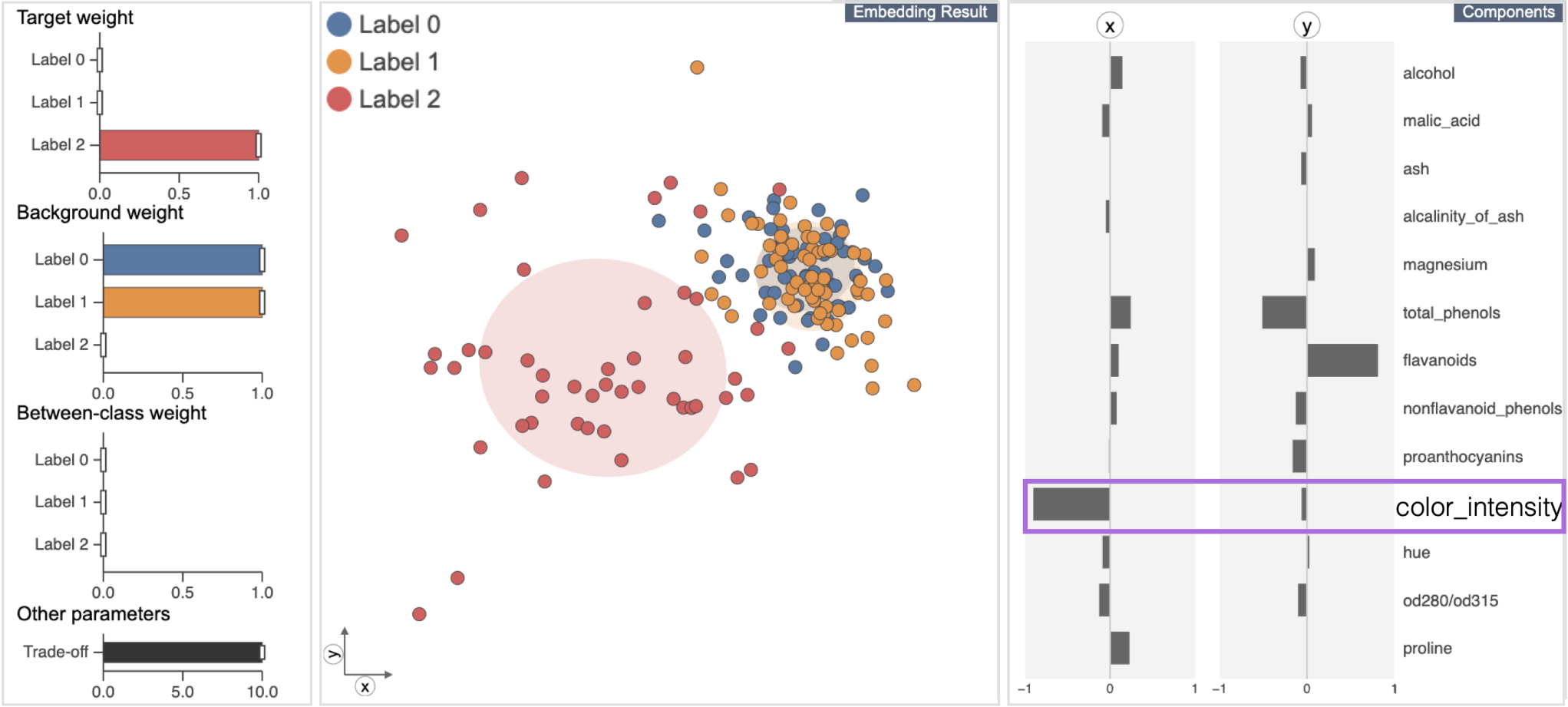
We further want to know factors that wines in Label 2 have a high variety than the others. To achieve this, we update parameters with the sliders in \autoreffig:uia so that the variance of Label 2 is maximized while minimizing the variances of Labels 0 and 1. The result is instantaneously updated, as shown in \autoreffig:example2, where we can see Label 2 has a much higher variance than the others along -axis. From \autoreffig:example2, we observe that color_intensity has a prominent influence on -axis; thus, Label 2 seems to consist of the wines with various color brightness.
The above analysis with the typical workflow presents that our framework provides flexible analysis and helps identify multiple characteristics of groups. Such flexibility and capability are not supported by existing methods, such as LDA and cPCA.
3 Methodology
This section introduces the design and derivation of ULCA in detail. \autoreftable:notation summarizes the notations used throughout the paper.
3.1 Existing Linear DR Used for Comparative Analysis
Since ULCA unifies several linear DR methods, we start from a brief introduction to the related methods, specifically, PCA, cPCA, and LDA.
PCA. PCA [43] finds latent features which maximally capture the variance of a whole dataset in an embedding space. The optimization to identify such latent features from attributes () can be written as:
| (1) |
where is a covariance matrix of the original data (: the number of data points) and is a projection matrix (note: is a identify matrix). This optimization is often solved with singular value decomposition, eigenvalue decomposition (EVD), or manifold optimization [4] (we describe the details in \autorefsec:optimization).
cPCA. cPCA [30, 2] is a variant of PCA for contrastive learning. Contrastive learning [99] aims to find salient features in one group (target group) by comparing it with another group (background group). Within this scheme, cPCA specifically finds latent features, with which a target group has a high variance but a background has a low variance (i.e., the saliency is identified in variance). This optimization can be written as:
| (2) |
where , are covariance matrices of target and background groups , , respectively (, : the number of data points in each group). is a hyperparameter, called a contrast parameter, which controls the trade-off between having a high target variance and a low background variance. When , cPCA only maximizes the variance of (i.e., PCA on ). As increases, cPCA more focuses on reducing the variance of .
cPCA is used for finding patterns hidden by dominant variance from features that do not relate to analysis interests (examples are provided by Abid and Zhang et al. [2]). In addition to this original usage (i.e., eliminating the influence from uninterested variations), cPCA can be used to compare two groups and to find more variety patterns in one group, such as political opinions diverse in supporters of a certain political party but uniform in the other supporters [27].
LDA. LDA [47] uses predefined group/class information to find an embedding that maximizes separation among groups. To do so, LDA minimizes data variance within each group while maximizes the separation of each group’s centroid. The optimization of LDA can be written as:
| (3) |
where and are within-class and between-class covariance matrices. These are computed with , where is the -th row of the input data , is the column means of , and is the column means of data points in a class that belongs to. Here, (: the number of classes or groups) is the -th element of , a vector containing a group label for each data point.
3.2 Unified Linear Comparative Analysis (ULCA)
Here, we introduce ULCA, which unifies and enhances cPCA and LDA. ULCA embraces functionalities of various linear DR methods, including PCA, cPCA, LDA, among others. As the intermediate product of ULCA, we introduce a generalized version of cPCA (gcPCA), which enables analysts to apply cPCA to any number of groups.
3.2.1 Generalization of cPCA
We generalize cPCA, which originally compares only two groups. Assume we have groups and let be a covariance matrix of data points in group , i.e., where when , otherwise . With weights and , of which -th elements and () represent contributions of group ’s covariance to target and background variances, the optimization problem of gcPCA can be written as:
| (4) |
Using and , gcPCA allows any groups to be target or background. For example, when , , and , \autorefeq:gcpca reduces to cPCA (\autorefeq:cpca), where groups 1 and 2 are target and background, respectively. It is noteworthy that when , , and , \autorefeq:gcpca reduces to ccPCA [26], which is an enhanced version of cPCA developed for characterizing clusters identified in the DR result. Moreover, with decimal weights, gcPCA can precisely control the effect from each group variance to an embedding.
| , , , | # of data points, original attributes, latent features, groups/classes. |
|---|---|
| , , | Original dataset, group labels of data points, embedding result. |
| Projection matrix. | |
| , | -th group’s within-class and between-class covariance matrices. |
| , , | Weights for target, background, between-class covariance matrices. |
| Trade-off parameter (or contrast parameter). | |
3.2.2 Trace-Ratio Form of gcPCA
LDA and gcPCA have a different form of the optimization problem with each other (refer to \autorefeq:lda and \autorefeq:gcpca). To enable integration of gcPCA and LDA, we introduce the trace-ratio form [49] of gcPCA.
As shown in \autorefeq:cpca and 4, cPCA and gcPCA’s optimization problems are written as the trace-difference problem (i.e., maximizing the difference of matrix traces) [49]. As discussed by Fujiwara et al. [28], when we want to maximize the variance of the target matrix while simultaneously minimizing the variance of the background matrix, the optimization problem of cPCA can be converted into the maximization of , which is the trace-ratio problem (i.e., maximizing the ratio of matrix traces). Similarly, for the same purpose, gcPCA can be written as the following trace-ratio problem:
| (5) |
As proved by Guo et al. [37], the optimization problem of \autorefeq:gcpca_trace_ratio is equivalent to find that produces zero as the optimum value of \autorefeq:gcpca. We describe an algorithm to find such in \autorefsec:optimization. Here, we want to note that we can regard gcPCA with \autorefeq:gcpca as a relaxed problem that finds with the user-specified . Now, we can handle both LDA (\autorefeq:lda) and gcPCA (\autorefeq:gcpca_trace_ratio) as the trace-ratio problem.
3.2.3 Integration of gcPCA and LDA
We introduce the optimization problem of ULCA by integrating gcPCA and LDA. By comparing \autorefeq:lda and \autorefeq:gcpca_trace_ratio, we can see that gcPCA and LDA share the same denominator when for all . However, gcPCA and LDA have slightly different numerators, where gcPCA and LDA have within-class and between-class covariance matrices, respectively. We can fill the gap between gcPCA and LDA by setting the following optimization problem:
| (6) |
| (7) |
| (8) |
where is a between-class covariance matrix related to group , i.e., ; () is the -th element of a vector ; and are non-negative numbers.
We use and to avoid the case where either matrix trace of or is always zero. While ULCA uses and by default, is used when and is used when . With this way, \autorefeq:ulca can handle either case where both and are zero vectors or is a zero vector. For example, when , , , \autorefeq:ulca only maximizes the within-class variance of group 1 (i.e., PCA to group 1). We use and mainly for the above purpose; however, similar to regularized LDA [36], these values can be used to add regularization terms for the case when is (close to) singular, which is usually caused when . Similar to other machine learning algorithms (e.g., linear regression), and can be used to add the bias into and to avoid overfitting.
By using ULCA, we can perform comparative analysis utilizing the strengths of both discriminant analysis and contrastive learning. For example, when , , and , ULCA produces the result where group 1’s variance and a distance between each group are maximized while the other groups’ variances are minimized. We demonstrate concrete analysis examples in \autorefsec:case_studies.
Similar to the discussion in \autorefsec:trace_ratio_form_gcpa, a relaxed ULCA, where is found with the user-specified , also can be written as:
| (9) |
After obtaining by solving \autorefeq:ulca or \autorefeq:ulca_trace_diff, embedding result can be generated from the original dataset with .
In summary, the optimization problems in \autorefeq:ulca and 9 are designed for ULCA, where the problems of gcPCA and LDA are integrated. Consequently, ULCA encompasses functionalities of PCA, cPCA, ccPCA, gcPCA, and (regularized) LDA while enabling flexible comparative analysis using discriminant analysis and contrastive learning together.
3.2.4 Optimization
We explain two approaches to solve \autorefeq:ulca and 9: using eigenvalue decomposition (EVD) and manifold optimization [87].
EVD-based approach. EVD is commonly used to solve the trace-difference problem [49]. that satisfies \autorefeq:ulca_trace_diff can be obtained by first applying EVD to and then taking the top eigenvectors.
To heuristically solve the trace-ratio problem of \autorefeq:ulca, we can use an iterative algorithm due to the work by Dinkelbach [18]. The algorithm consists of two steps. Given at iteration step , we perform
| (10) | ||||
| (11) |
At , because the computed does not exist, we self-define as a default solution to Step 1. As demonstrated, in \autorefeq:iter_step1 is an objective value of \autorefeq:ulca, which is computed with the current . The second step (\autorefeq:iter_step2) is to derive for the next iteration. This step just solves the relaxed problem (\autorefeq:ulca_trace_diff) based on the current parameter with EVD. With this iterative algorithm, monotonically increases till ‘’ reaches approximately zero and usually converges quickly (e.g., in less than 10 iterations) [28, 49].
Manifold-optimization-based approach. Another way to solve \autorefeq:ulca and \autorefeq:ulca_trace_diff is using a generic solver designed for optimization over manifolds (or often called manifold optimization) [4]. According to Cunningham and Ghahramani [17], linear DR can be considered as solving a manifold optimization problem. We can also directly solve both \autorefeq:ulca and \autorefeq:ulca_trace_diff with a manifold optimization solver available in existing libraries, such as Manopt [10]. More specifically, using the Riemannian Trust Regions (RTR) method [3] over the Grassmann manifold can be used as a solver to achieve the best performance due to the evaluation by Cunningham and Ghahramani [17]. Refer to their work [17] for details of manifold optimization and solvers.
When compared with the EVD-based approach, manifold optimization has two main benefits. First, manifold optimization is generic for linear DR methods, including methods that cannot be represented as the trace-ratio or trace-difference problem. As a result, when adding some enhancement to ULCA in the future, we just need to design a new optimization problem and do not need to find a solution specific to the new problem. Also, while EVD captures more information in the top eigenvectors than others (e.g., the first eigenvector preserves the original data variance than the second eigenvector), manifold optimization equally treats each embedding axis. This is especially beneficial when we use DR for a visualization purpose as we can fully utilize a 2D space to convey the preserved information. Therefore, our implementation of ULCA, by default, uses manifold optimization with the RTR method [3] while we provide the EVD-based approach as an option.
ULCA’s embedding axes (i.e., columns of ) obtained via manifold optimization are always orthogonal but could have a different rotation at every execution (even with the same dataset and parameters). To produce consistent axes, by default, we apply the varimax rotation [56] to . This rotates to minimize the number of attributes that have a high contribution to the axes; thus, it can also improve the interpretability of axes, as often used in factor analysis [54]. However, the varimax rotation still does not produce consistent axes in terms of their order and sign. Thus, we adjust the signs to make each column sum of positive, and reorder the axes by the maximum column value of .
3.3 Parameter Selection
ULCA allows analysts to adjust multiple important parameters: , , , and . Here, we provide general guidance on how to chose desired parameters. Also, as a convenient way to select parameters, we introduce the backward parameter selection, which finds the best parameters to resemble the changes indicated in an embedding result.

3.3.1 General Guidance
A general rule of parameter selection is simple. When we want to observe higher variances in some groups, for the corresponding groups, we should set larger weights in and smaller weights in , and vice versa. When we want to increase a distance between groups, we should assign larger values to the corresponding weights in . can be selected automatically by solving \autorefeq:ulca. However, as demonstrated in the analyses using cPCA by Abid and Zhang et al. [2], using a different in \autorefeq:ulca_trace_diff may lead to the discovery of latent patterns that could not be found with an automatically selected value. can be used to control how much the background variance should be reduced in an embedding result (i.e., larger , smaller background variance).
In \autoreffig:param_select, we demonstrate several examples using different parameters. \autoreffig:param_selecta uses parameters that produce the same result with LDA and is automatically selected. From \autoreffig:param_selecta, for example, by decreasing , we can weaken the reduction of the orange group’s variance relative to others, as shown in \autoreffig:param_selectd. Another example in \autoreffig:param_selectb is generated by reducing and ; consequently, only the red group has clear separation from others. \autoreffig:param_selecte uses smaller than \autoreffig:param_selectb, and it changes the variance relationships. In \autoreffig:param_selectc, is increased and is reduced. As a result, the red group gets a much larger variance. Lastly, we set small relative to in \autoreffig:param_selectf. The orange group’s variance is now larger than that of the blue group.
3.3.2 Backward Parameter Selection
As discussed above, once we know how each parameter influences an embedding result, it is not difficult to select proper parameters based on analysis purposes. However, to further aid parameter selection, we develop a backward algorithm that finds parameters to resemble a user-demonstrated change in a visualized result [82]. The backward algorithm supports two types of changes or interactions: (1) moving a group centroid and (2) scaling a group variance in an embedding result. These two interactions are closely connected to possible user intents [84, 83, 93] in comparative analysis. The first interaction infers that the analyst wants to change distance relationships among groups, for example, to find better group separation. With the second interaction, the analyst intends to change relative variances among groups, for example, to increase a certain group’s variance relative to the others.

fig:backward_param_select shows examples of the backward parameter selection when the two interactions are performed. For scaling of a group variance, instead of adjusting each group variance directly, we change the variance through uniform-scaling of the confidence ellipse as it is commonly used to visualize the scatteredness of data points. After either interaction is performed, the backward algorithm should find parameters so that both relative centroid distances and relative variance differences of each group in the demonstrated changes (e.g., \autoreffig:backward_param_selecta2, b2) are preserved as much as possible. Such optimization can be written as:
| (12) |
| (13) |
| (14) |
where consists of parameters, , , , and ; and () are cost functions related to the distance and variance relationships, respectively; is a label of moved/scaled group (); and (, ) are parameters that control the weights of and to the total cost. And, .
can be computed with the user-indicated centroid distances () and new centroid distances , which are generated with parameters . As shown in \autorefeq:cost_dist, we follow classical MDS’s strain [86] to design , where the root sum squared (RSS) of distance differences is computed and scaled to a range of . We compute with (), the areas of the user-indicated confidence ellipses, and , the areas of the confidence ellipses in a new embedding space. In \autorefeq:cost_area, we first compute and (the moved/scaled group’s area ratios to the other) and then take their sum of absolute differences (SAD). Afterward, we scale the SAD to a range of . From and , we compute the total cost with and . We can set different and for each interaction. When moving a centroid, we expect that the analyst mainly wants to refine the distance relationships, and thus, we use and by default. On the other hand, for the scaling, we use and .
Now, we need to solve \autorefeq:backward_algorithm to find the optimal . Since and are obtained after solving \autorefeq:ulca_trace_diff, this problem is optimizing over the optimization of \autorefeq:ulca_trace_diff. As a result, it may be difficult to find a direct solution, such as using EVD, or to derive a gradient. Thus, we use a generic gradient-free solver. Also, we need to constrain all the weights of , , within a range of and within . To satisfy these requirements, we select COBYLA (or constrained optimization by linear approximations) [77]. For each iteration of the optimization with COBYLA, we solve \autorefeq:ulca_trace_diff with given and compute the cost in \autorefeq:backward_algorithm. Then, COBYLA selects a new from a trust region for the next iteration. COBYLA keeps iterating these steps until reaching the convergence or specified maximum number of iterations. We provide an evaluation of the optimization using COBYLA in \autorefsec:perf_eval.
3.4 Complexity Analysis
We first analyze the time complexity of ULCA when using the EVD-based approach. If , which is a reasonable assumption for a practical usage, the relaxed version of ULCA in \autorefeq:ulca_trace_diff has two major calculations: covariance matrix calculation () and EVD (). Thus, the relaxed version of ULCA has time complexity, which is compatible with PCA and cPCA. As mentioned, solving \autorefeq:ulca with the iterative algorithm converges quickly. Thus, the complexity of the non-relaxed version of ULCA is similar to .
After the covariance matrix calculation (), the manifold-optimization-based approach iteratively solves \autorefeq:ulca or \autorefeq:ulca_trace_diff with a manifold optimization solver. Each iteration performs matrix multiplication of and covariance matrices, which has the time complexity of , and then computes partial derivatives for the next iteration. When using the RTR method [3], at each iteration, the second-order partial derivatives (or the Hessian matrix) are computed with time complexity. When , we can consider both of the above time complexities are . Now, the time complexity depends on the number of iterations till the convergence. Based on the performance evaluation by Cunningham and Ghahramani [17], the manifold optimization runtime for various linear DR methods follows approximately three orders of . From this, we can consider that the manifold-optimization-based approach practically has a similar runtime to the EVD-based approach. However, in the worst case, as studied by Boumal et al. [9], the RTR method needs to iterate where () is the convergence threshold. To avoid a numerous number of iterations, we can also set the maximum number of iterations. For example, to complete the optimization in similar runtime with the EVD-based approach, we can use as the maximum number of iterations.
The backward parameter selection in \autorefsec:param_optim solves \autorefeq:ulca_trace_diff at each iteration with parameters selected by COBYLA [77]. Thus, the time complexity is the multiplication of the user-specified maximum number of iterations and ULCA’s time complexity.
4 Visual Interface
Our framework provides a visual interface to visualize and interact with a ULCA result. As shown in \autoreffig:ui, the interface provides three views with simple visualizations: (a) a parameter view, where bar charts display parameters of , , , and ; (b) an embedding result view, where a scatterplot depicts an embedding result with the confidence ellipse of each group; (c) a component view, where bar charts show the information of the axes of the embedding result view. All views are fully linked, and each is updated based on an interaction performed in the other views.
Supported interactions. In the parameter view (\autoreffig:uia), the analyst can adjust each parameter by changing the corresponding bar length. This interaction instantly reruns ULCA in \autorefeq:ulca_trace_diff. In the embedding result view (\autoreffig:uib), the analyst can move each group’s centroid and scale each confidence ellipse by dragging the corresponding confidence ellipse’s center and outline, respectively. These changes induce the backward parameter selection. The analyst also can draw a new axis, as demonstrated with axis \small1⃝ in \autoreffig:uib, to see how each attribute contributes to directions of interest. A linear mapping from the original attributes to the new axis can be computed with where is a vector of the new axis. Then, this information is added to the component view. When hovering over a certain attribute name in the component view (\autoreffig:uic), to see the distribution of the attribute values, each point’s size in the embedding result view is updated based on its attribute value.
Mental map preservation. When updating an embedding, linear DR methods that use EVD or manifold optimization, including ULCA, cause arbitrary sign flipping and rotations of embedding axes [25]. Thus, an embedding result would be drastically changed, and it would be difficult to follow the changes as the analyst easily loses their mental map [78]. To mitigate this problem, we take an approach similar to one developed to use linear DR in a streaming setting [25] (note that several works addressed mental map preservation for nonlinear DR [80, 13]). We use the rotation matrix obtained through the Procrustes analysis [34] of the previous and new embedding results. This rotation matrix adjusts the new embedding axes’ signs and rotations to minimize the difference of data positions from the previous result. Furthermore, we animate the changes in each view to help the analyst maintain their mental map.
Provenance support. During the interactive analysis, the analyst may find interesting patterns and may want to record the (intermediate) analysis results to further investigate the results by comparing with other results later, apply the obtained embedding to other data, or share the results with others. To help the analyst keep the history of changes during the analysis (or called provenance [79]), we provide a saving function. The analyst can name the result and save it through the text input field and the ‘save’ button placed at \autoreffig:uid. This function saves all necessary information to recover both visualizations and ULCA results. The analyst can go back to the saved result by selecting the corresponding name from the drop-down list of the saved names (the left side of \autoreffig:uid). Also, the saved results can be directly referred from Python and the Jupyter Notebook due to the seamless integration of the interface with them, as described below.

4.1 Implementation
The knowledge discovery process often requires many different analytical components [24, 58]. To allow for use of ULCA together with all necessary algorithms, visualizations, and interactions, we design the visual interface to be seamlessly used with Python and the Jupyter Notebook [60]. In this way, when analyzing datasets with our framework, the analyst can utilize various existing analysis and visualization libraries, such as scikit-learn [73] (for machine learning), Matplotlib [46] (for visualization), or their own analysis methods. Also, the analyst can employ various analytical processing, such as assigning new labels to data points and sorting the attributes in the component view based on their contributions to each embedding axis. In \autoreffig:ui, we visualize the result obtained by applying ULCA to the processed dataset in the Jupyter Notebook, interact with the result in the visual interface, and access the information gained through interactive analysis.
fig:system_architecture shows our framework’s system architecture. While the front end is implemented as a web-based application with JavaScript and D3 [8], the other parts are implemented with Python. For the implementation of optimization solvers, the framework uses Pymanopt [87] and SciPy [90]. To make the front end callable from the Jupyter Notebook’s code cells where we can write and run Python scripts, we implement a plotting module that consists of a controller, servers, and the front end.
The analyst can use the controller to adjust settings and call the visual interface, as demonstrated in ‘In [5]’ code cell in \autoreffig:ui. Then, the controller starts HTTP and WebSocket servers in localhost to establish communications. Afterward, the visual interface is shown by using an HTML inline frame, as shown in ‘Out [5]’ in \autoreffig:ui. All the information shown in the visual interface is stored in the plotting module as Python objects, and can be accessed via the controller. For example, ‘In [6]’ in \autoreffig:ui refers to -axis information of the current result shown in ‘Out [5]’ and that of the saved result named with ‘PCA on Label 1’. The controller provides an option to show the visual interface in an individual webpage (the dashed lines and boxes in \autoreffig:system_architecture). The framework also can be used without using the Jupyter Notebook.
5 Performance Evaluation
We evaluate the performance of ULCA and the backward parameter selection. As an experimental platform, we use the MacBook Pro (16-inch, 2019) with 2.3 GHz 8-Core Intel Core i9 and 64 GB 2,667 MHz DDR4. The experiment details are available online [1].
Data. We generate datasets with various numbers of data points, attributes, and groups. From the documents (i.e., data points) in the 20 Newsgroups dataset [21], we extract arbitrary numbers of topics (i.e., attributes) by utilizing the Latent Dirichlet Allocation [6]. To obtain various numbers of data points and groups, we randomly sample documents and apply -means clustering [39] to the sampled documents.
Evaluation of ULCA. We evaluate the efficiency of the relaxed (\autorefeq:ulca_trace_diff) and non-relaxed (\autorefeq:ulca) versions of ULCA, using EVD (EVD) and manifold optimization (Man). For each different combination of the numbers of data points () and attributes (), we execute ULCA 10 times with random values of , , and compute the average completion time. We use a fixed number of groups () because it does not have a strong influence on the computational cost. For the relaxed version of ULCA, we use . The result is shown in \autoreffig:perf_eval_ulca.
From \autoreffig:perf_eval_ulca, no matter what version and approach are used, the completion time mainly depends on the number of attributes. However, even for a large number of attributes, ULCA can be solved quickly. For example, the relaxed and non-relaxed versions are solved about 1 second when and , respectively. From the comparison of EVD and Man, EVD is faster when the number of attributes is relatively small while Man becomes similar or faster than EVD after . This tendency is more apparent in \autoreffig:perf_eval_ulcab. As described in \autorefsec:complexity, EVD’s time complexity heavily depends on the number of attributes (scale of ). Man is less sensitive to it (scale of ). One notable point is the dramatic time increase when and for both EVD and Man in \autoreffig:perf_eval_ulcab. We consider that this is due to the instability of LDA’s optimization when , as studied by Guo et al. [36]. Since ULCA inherits the characteristics of LDA, ULCA also suffers from the same problem. Consequently, the iterative steps used in both EVD and Man cannot reach the convergence quickly. To avoid this, similar to the work by Guo et al. [36], we can apply regularization with and .

Evaluation of the backward parameter selection. We test the completion time and accuracy of the backward parameter selection. We use only the manifold-optimization-based approach and a fixed number of data points (i.e., ) but various values for the maximum number of iterations for COBYLA (here, we represent it with ), number of groups , and number of attributes . Other parameters are set with default values. For each setting, we generate an initial embedding result with and random values of , , . Then, we mimic the user-demonstrated change in the initial embedding result by randomly selecting a group and an interaction (e.g., moving group 1’s centroid to coordinate or expanding group 2’s confidence ellipse times) and the backward parameter selection is performed for this mimicked change. We generate 500 sets of changes for each setting and compute the average completion time and accuracy. The accuracy is calculated with where , , and are the cost of \autorefeq:backward_algorithm when using the initial embedding, fully optimized parameters, and parameters produced with , respectively. We set the objective value obtained with as . The case where indicates there is no way to refine the embedding; thus, we discard such cases. The result is shown in \autoreffig:perf_eval_backward.
From \autoreffig:perf_eval_backwarda, the completion time linearly increases by . In \autoreffig:perf_eval_backwardb, the accuracy is clearly improved till reaches or ; however, afterward, clear improvement cannot be seen. From this, we can consider that the optimization can often produce a sufficient solution at around 40th iterations. Also, the optimization is finished within about 1 second when and 2 seconds when . Thus, we can set about 20 when we need more interactivity, otherwise, we can set it about . However, when the number of groups is large (e.g., ), the accuracy could be low (e.g., 0.6), as shown in \autoreffig:perf_eval_backwardb. In such cases, we can consider using larger while sacrificing the interactivity.
In summary, our evaluation shows the high efficiency of ULCA: the completion time is about 1 second even when and . Thus, we can instantaneously update ULCA when adjusting parameters in the visual interface. The background parameter selection also can provide a sufficient result in a considerably short time (e.g., 80% of accuracy in 2 seconds). The results guide selection of solvers (e.g., EVD vs Manopt) and parameters (especially, the maximum number of iterations in COBYLA) for better performance and interactive usage.
6 Case Studies
We have demonstrated the usefulness of our framework by analyzing the Wine dataset [21] in \autorefsec:workflow_and_example. With publicly available data, we perform two additional case studies. All detailed information of the data (e.g., details of the survey questions in \autorefsec:cs1), analysis processes, used parameters, and results are available at our website [1].
6.1 Case Study 1: Analysis of Political Groups
We analyze the PPIC Statewide Survey, October 2018 [5]. This survey contains California residents’ political opinions on, for example, political parties and expansion of the Mexico-U.S. barrier. By comparing groups within this dataset, such as supporters of different political parties, we can identify their opinion differences or reveal subgroups within each group. As a representative analysis, we look for a subgroup within the Democrat supporters (Dem) by comparing them with the Republican supporters (Rep), and review the characteristics of the subgroup.
In the Jupyter Notebook, we first preprocess the dataset to select data points (i.e., residents) and attributes (i.e., survey questions) of interest, discard missing values, and apply normalization to each attribute. Note that while most of the attributes are either binary, ordinal, or numerical, we drop nominal data because it is not suitable to be analyzed with ULCA. In the end, 548 data points and 27 attributes remain.
We then use ULCA with parameters that produce the same result when applying cPCA to Dem and Rep as target and background groups, respectively. This setting reveals opinions that are varied in Dem but uniform in Rep. With the visual interface, we initially display the ULCA result with , and interactively increase the value until we find interesting patterns, resulting \autoreffig:cs1a where . In \autoreffig:cs1a, Dem is separated into both left and right sides, while Rep is mostly placed at the right-hand side. As shown in the component view, -axis is dominantly constructed from Q30, which asks if they have a favorable impression of the current Democrat party. By hovering over Q30 in the view, we can see that Dem has both supporters who do and do not have a favorable impression of the Democrats. Note that we easily found this result because of exploratory data analysis using DR. For example, the Mann-Whitney U rank test on Dem and Rep for each question reveals that most questions (20 of 27) have a statistically significant difference. This information is not useful to find the subgroups of Dem. Also, without interactively adjusting and looking at \autoreffig:cs1a, finding the Dem’s subgroup overlapping with Rep is difficult.
To investigate more of the residents who support the Democrats but do not have a favorable impression, we write a script in the Jupyter Notebook to separate Dem based on the answer for Q30: Dem(+) (the answer is ‘yes’) and Dem(-) (‘no’), and drop Q30 from the attributes. Then, we apply ULCA with parameters that highlight opinions that are more varied in Dem(-) than Dem(+) and Rep. The result in \autoreffig:cs1b successfully reveals such opinions (i.e., Dem(-) has a higher variance than others). Unlike \autoreffig:cs1a, many attributes significantly contribute to the axes, such as Q1 (whether Jerry Brown’s performance as the California governor is appropriate or not) and Q25 (whether the gun restriction should be more strict or not). As an example, we select Q1 in \autoreffig:cs1b, where Dem(+) (blue) and Rep (red) have almost uniform opinions on Brown’s performance (Dem(+): positive, Rep: negative opinions) while Dem(-) consists of both opinions. Through this analysis, we can expect that those in Dem(-) have objections to some Democrats’ policies, leading to an unfavorable impression of the current party.
Next, we identify political opinions that can clearly distinguish Dem(+) and Rep but are diverse within Dem(-). To achieve this, we interactively move away Rep and Dem(+)’s centroids from each other in the interface. The backward parameter selection then automatically finds the proper parameters to refine the result, as shown in \autoreffig:cs1c. At this time, Q20 (annotated with a purple box) and Q21a (orange box) most contribute to - and -axes, respectively. Q20 asks if they approve of Donald Trump’s performance as the president while Q21a is about their opinion on Trump’s nomination of Brett Kavanaugh to the U.S. Supreme Court. Thus, both questions are highly related to how the residents think about Donald Trump. We select Q20 from the component view. As shown in \autoreffig:cs1c, the majority of Dem(+) does not approve Trump’s performance. However, a considerable amount of people in Dem(-) appreciate the work by Donald Trump.

6.2 Case Study 2: Characterizing Handwritten Digits
We analyze the MNIST handwritten digits dataset [64]. This dataset contains 70,000 handwritten digits (i.e., data points) stored in pixels (i.e, 784 attributes). Here, we review each digit’s characteristics by comparing it to other digits. More specifically, we compare digits 0, 6, and 9, all of which have a similar rounded structure.
We first sample 500 images for each digit to moderate visual clutter in a resultant embedding space. To understand the various structures that people write for 6 and 9 but not for 0, we use ULCA to maximize 6 and 9’s variances while minimizing 0’s variance in the embedding space. The result in \autoreffig:cs2a shows that digit 9 has a much higher variance than 6. This implies the embedding mainly captures the information related to 9. To produce similar variances for both 6 and 9, we interactively reduce 9’s weight in . In \autoreffig:cs2b, when we halve the corresponding weight, digits 6 and 9 achieve a similar variance. Also, we can see that 9 and 6 are widely distributed along - and -axes, respectively.
To understand structures highly related to the spread along each axis, we refer to each pixel’s contribution to the construction of each axis. However, since we have many pixels and want to see the contribution information in the context of digit shapes, the component view is not suitable for this analysis. As we can seamlessly access all the information in the visual interface, we extract the axis information and depict it in 2D heatmaps (the right side of \autoreffig:cs2b) with an external visualization library. From the heatmaps, we can see how people tend to write each digit differently. For example, as annotated with \small1⃝ and \small2⃝, digit 9 is written typically in two ways with a straight line, which cannot be seen in digit 0. For digit 6, we observe that people tend to use either of the strokes annotated with \small3⃝ and \small4⃝ to make 6 different from 0. However, 6 is overlapped with 0 at the bottom left in the embedding space, where we expect 6 is written with the stroke annotated with \small3⃝.
We move on to finding strokes that clearly differentiate 6 and 9 from 0 but are still written variously for 6 and 9. These strokes characterize the uniqueness of 6 and 9 relative to 0. To see if we can separate 0 from the others in the embedding, we set 1 to 0’s weight in . Then, by gradually increasing , we find the desired embedding (\autoreffig:cs2c), where 0 has almost no overlap with the others. As seen in the heatmaps in \autoreffig:cs2c, while the new -axis is similar to the previous one, the new -axis is highly influenced by the pixels annotated with \small{5}⃝. This implies that the corresponding pixels tend to be used only when writing digit 6 or 9, but the amount of these pixels used for 6 or 9 differs by person.
Lastly, because we expect that the strokes annotated with \small1⃝ and \small2⃝ are also used for other digits, such as 1, 4, and 7, we are interested in whether the patterns similar to 9 can be found (or not found) for these other digits. By using the projection matrix used for \autoreffig:cs2c, we plot the sampled 500 data points of digit 7 onto the same embedding space. From the result shown in \autoreffig:cs2d, we can see that 7 has a similar distribution as 9 along -axis in general; however, 7 is clustered more on the left-hand side of the embedding space, as annotated with yellow. This annotated part tends to use the diagonal stroke \small{1}⃝ in \autoreffig:cs2b. Thus, when writing 7, people often use the diagonal stroke \small{1}⃝ more and the vertical stroke \small{2}⃝ less when compared to writing 9.
This case study demonstrates how the embedding results can guide the analysis (e.g., the parameter adjustment after looking at the variance difference between 6 and 9 in \autoreffig:cs2a) and how the component/axis information can help analysts find patterns rooted in the combination of multiple attributes (e.g., the strokes shown in \autoreffig:cs2b).

7 Discussion
We demonstrate the usefulness of our framework for comparative analysis with our case studies, where we use the collective power of discriminant analysis, contrastive learning, and interactive refinement of DR results. These demonstrative analyses highlight the potential usage of our framework for a variety of applications. The patterns found in the case studies are difficult to identify with other DR methods, such as PCA, LDA, and cPCA. For example, as shown in \autoreffig:lda_cpca, while applying LDA and cPCA to the dataset used in Case Study 2 can reveal clusters for digits 0, 6, and 9, we cannot find interesting patterns from the information of components unlike what ULCA provides. We provide a comprehensive comparison among ULCA and other methods in the supplementary material [1]. Our algorithms’ performance is also discussed in \autorefsec:perf_eval. Here, we further discuss other aspects of our framework.
Visualization design. The design of our visual interface aims to keep visualizations as simple as possible and only use visualizations that most analysts are likely to be familiar with. However, at the same time, this design choice may cause problems, such as visual scalability. For example, in the parameter view, we assign an individual bar chart for each group’s weight and a different color for each group; consequently, the related visualizations are not scalable to a large number of groups. Similarly, the component view is not scalable for a dataset with a large number of attributes. However, due to the seamless integration with Python, we can easily use alternative visualizations, as demonstrated in the case study. Ideally, the visual interface should allow the analysts or visualization developers to customize views based on their analysis needs. We plan to extend our implementation to be applicable to any visualizations developed with D3 into the visual interface.
Parameter suggestion. The backward parameter selection finds parameters that resemble the user-demonstrated change as close as possible. However, the analyst may try infeasible refinements. For example, they might try to increase some group’s variance even when its variance is already maximized. To avoid this, similar to the feasibility map by Cavallo and Demiralp [14], we could precompute embeddings derived with various potential interactions and inform which interactions are feasible. However, this approach has a drawback in its computational cost as we need to check the feasibility from the wide searching space. Another interesting approach is suggesting which parameter values can result in significantly different embedding results when compared to other cases. For this approach, we can employ several existing methods [2, 66]. For example, for cPCA, Abid and Zhang et al. [2] suggested a small set of contrast parameter values (e.g., 4 values) by applying spectral clustering to the embedding results generated with many values (e.g., 40 values). This approach, though, also would have a large computational cost as ULCA has many adjustable parameters. We will investigate how we can achieve the recommendation of interactions or parameters to find interesting embedding patterns in the future.
Characteristics of ULCA. ULCA is a tool for exploratory data analysis. Similar to the discussion on cPCA by Abid et al. [2], while ULCA uses group labels for embedding, ULCA is different from other supervised learning methods that focus on a task of classification/regression and multi-group statistical hypothesis tests whose primary goal is identifying an attribute that has a significantly different statistic value (e.g., mean) in each group. ULCA is a linear DR method, which can extract a latent linear structure from high-dimensional data. ULCA benefits from the linearity to provide interpretable embedding axes; however, the linearity also might limit ULCA’s capability to find patterns when analyzing complex data. We plan to investigate how to extend ULCA to a nonlinear DR method while retaining interpretability. Another limitation of ULCA is interpreting the result could be still difficult when analyzing a dataset with a very large number of attributes (e.g., 1,000 attributes) even with the axis information. When applying ULCA to such a dataset, many of the attributes (e.g., 100 attributes) could significantly contribute to embedding axes. To avoid using many attributes when constructing the embedding axes, various sparse DR methods, such as sparse PCA [98], sparse LDA [15], and space cPCA [7], have been developed. These methods produce a sparse projection matrix by penalizing a case where an embedding uses many attributes. We also plan to extend ULCA to a sparse DR method.
8 Conclusion
We have developed an interactive DR framework by introducing a new DR method, ULCA, which uses the collective capability of discriminant analysis and contrastive learning. The framework further supports interactive analysis with a visual interface that can be seamlessly used with existing analysis libraries and also with an optimization algorithm that can interactively refine ULCA results. This new DR framework makes a tangible contribution to comparative analysis.
Acknowledgements.
The authors wish to thank Dr. Tzu-Ping Liu at the University of Taipei and Samuel Fuller at UC Davis for their guidance for the dataset used in Case Study 1. This work is supported in part by the U.S. National Science Foundation through grant IIS-1741536, the U.S. National Institute of Standards and Technology through grant 70NANB20H197, and the Natural Sciences and Engineering Research Council of Canada.References
- [1] The supplementary materials: The demonstration video of the framework, source code, evaluation details, and supplemental evaluation. \urlhttps://takanori-fujiwara.github.io/s/ulca/.
- [2] A. Abid, M. J. Zhang, V. K. Bagaria, and J. Zou. Exploring patterns enriched in a dataset with contrastive principal component analysis. Nat. Commun., 9(1):2134, 2018.
- [3] P.-A. Absil, C. G. Baker, and K. A. Gallivan. Trust-region methods on Riemannian manifolds. Found. of Comput. Math., 7(3):303–330, 2007.
- [4] P.-A. Absil, R. Mahony, and R. Sepulchre. Optimization algorithms on matrix manifolds. Princeton University Press, 2009.
- [5] M. Baldassare, D. Bonner, A. Dykman, and L. Lopes. PPIC statewide survey: Californians & their government, October 2018. Report: \urlhttps://www.ppic.org/wp-content/uploads/ppic-statewide-survey-october-2018.pdf, Dataset: \urlhttps://www.ppic.org/data-set/ppic-statewide-survey-data-2018/, 2018. Accessed: 2021-3-21.
- [6] D. M. Blei, A. Y. Ng, and M. I. Jordan. Latent Dirichlet allocation. J. Mach. Learn. Res., 3:993–1022, 2003.
- [7] P. Boileau, N. S. Hejazi, and S. Dudoit. Exploring high-dimensional biological data with sparse contrastive principal component analysis. Bioinformatics, 36(11):3422–3430, 2020.
- [8] M. Bostock, V. Ogievetsky, and J. Heer. D3 data-driven documents. IEEE Trans. Vis. Comput. Graph., 17(12):2301–2309, 2011.
- [9] N. Boumal, P.-A. Absil, and C. Cartis. Global rates of convergence for nonconvex optimization on manifolds. IMA J. Numer. Anal., 39(1):1–33, 2019.
- [10] N. Boumal, B. Mishra, P.-A. Absil, and R. Sepulchre. Manopt, a Matlab toolbox for optimization on manifolds. J. Mach. Learn. Res., 15(1):1455–1459, 2014.
- [11] M. Brehmer, M. Sedlmair, S. Ingram, and T. Munzner. Visualizing dimensionally-reduced data: Interviews with analysts and a characterization of task sequences. In Proc. BELIV, pp. 1–8, 2014.
- [12] E. T. Brown, J. Liu, C. E. Brodley, and R. Chang. Dis-Function: Learning distance functions interactively. In Proc. VAST, pp. 83–92, 2012.
- [13] G. D. Cantareira and F. V. Paulovich. A generic model for projection alignment applied to neural network visualization. In Proc. EuroVA, 2020.
- [14] M. Cavallo and Ç. Demiralp. A visual interaction framework for dimensionality reduction based data exploration. In Proc. CHI, pp. 1–13, 2018.
- [15] L. Clemmensen, T. Hastie, D. Witten, and B. Ersbøll. Sparse discriminant analysis. Technometrics, 53(4):406–413, 2011.
- [16] D. B. Coimbra, R. M. Martins, T. T. Neves, A. C. Telea, and F. V. Paulovich. Explaining three-dimensional dimensionality reduction plots. Inform. Visual., 15(2):154–172, 2016.
- [17] J. P. Cunningham and Z. Ghahramani. Linear dimensionality reduction: Survey, insights, and generalizations. J. Mach. Learn. Res., 16(1):2859–2900, 2015.
- [18] W. Dinkelbach. On nonlinear fractional programming. Management Science, 13(7):492–498, 1967.
- [19] M. Dowling, J. Wenskovitch, J. T. Fry, S. Leman, L. House, and C. North. SIRIUS: Dual, symmetric, interactive dimension reductions. IEEE Trans. Vis. Comput. Graph., 25(1):172–182, 2019.
- [20] J.-B. du Prel, B. Röhrig, G. Hommel, and M. Blettner. Choosing statistical tests: Part 12 of a series on evaluation of scientific publications. Deutsches Ärzteblatt International, 107(19):343, 2010.
- [21] D. Dua and C. Graff. UCI machine learning repository. \urlhttp://archive.ics.uci.edu/ml, 2019.
- [22] A. Endert, C. Han, D. Maiti, L. House, S. Leman, and C. North. Observation-level interaction with statistical models for visual analytics. In Proc. VAST, pp. 121–130, 2011.
- [23] M. Espadoto, R. M. Martins, A. Kerren, N. S. T. Hirata, and A. C. Telea. Toward a quantitative survey of dimension reduction techniques. IEEE Trans. Vis. Comput. Graph., 27(3):2153–2173, 2021.
- [24] U. Fayyad, G. Piatetsky-Shapiro, and P. Smyth. From data mining to knowledge discovery in databases. AI Mag., 17(3):37–37, 1996.
- [25] T. Fujiwara, J.-K. Chou, S. Shilpika, P. Xu, L. Ren, and K.-L. Ma. An incremental dimensionality reduction method for visualizing streaming multidimensional data. IEEE Trans. Vis. Comput. Graph., 26(1):418–428, 2020.
- [26] T. Fujiwara, O.-H. Kwon, and K.-L. Ma. Supporting analysis of dimensionality reduction results with contrastive learning. IEEE Trans. Vis. Comput. Graph., 26(1):45–55, 2020.
- [27] T. Fujiwara and T.-P. Liu. Contrastive multiple correspondence analysis (cMCA): Using contrastive learning to identify latent subgroups in political parties. arXiv:2007.04540, 2020.
- [28] T. Fujiwara, J. Zhao, F. Chen, Y. Yu, and K.-L. Ma. Interpretable contrastive learning for networks. arXiv:2005.12419, 2020.
- [29] S. García, J. Luengo, and F. Herrera. Data Preprocessing in Data Mining, vol. 72. Springer, 2015.
- [30] R. Ge and J. Zou. Rich component analysis. In Proc. ICML, pp. 1502–1510, 2016.
- [31] M. Gleicher. Explainers: Expert explorations with crafted projections. IEEE Trans. Vis. Comput. Graph., 19(12):2042–2051, 2013.
- [32] M. Gleicher. Considerations for visualizing comparison. IEEE Trans. Vis. Comput. Graph., 24(1):413–423, 2018.
- [33] M. Gleicher, D. Albers, R. Walker, I. Jusufi, C. D. Hansen, and J. C. Roberts. Visual comparison for information visualization. Inform. Visual., 10(4):289–309, 2011.
- [34] J. C. Gower and G. B. Dijksterhuis. Procrustes Problems, vol. 30. Oxford University Press on Demand, 2004.
- [35] R. Guo, T. Fujiwara, Y. Li, K. M. Lima, S. Sen, N. K. Tran, and K.-L. Ma. Comparative visual analytics for assessing medical records with sequence embedding. Visual Informatics, 4(2):72–85, 2020.
- [36] Y. Guo, T. Hastie, and R. Tibshirani. Regularized linear discriminant analysis and its application in microarrays. Biostatistics, 8(1):86–100, 2007.
- [37] Y.-F. Guo, S.-J. Li, J.-Y. Yang, T.-T. Shu, and L.-D. Wu. A generalized Foley–Sammon transform based on generalized Fisher discriminant criterion and its application to face recognition. Pattern Recogn. Lett., 24(1-3):147–158, 2003.
- [38] C. Hare, D. A. Armstrong, R. Bakker, R. Carroll, and K. T. Poole. Using bayesian Aldrich-McKelvey scaling to study citizens’ ideological preferences and perceptions. Am. J. Polit. Sci., 59(3):759–774, 2015.
- [39] J. A. Hartigan and M. A. Wong. A k-means clustering algorithm. J. R. Stat. Soc. C-Appl.), 28(1):100–108, 1979.
- [40] T. Hastie and R. Tibshirani. Discriminant analysis by Gaussian mixtures. J. R. Stat. Soc. B, pp. 155–176, 1996.
- [41] J. Hill, W. R. Ford, and I. G. Farreras. Real conversations with artificial intelligence: A comparison between human–human online conversations and human–chatbot conversations. Comput. Hum. Behav., 49:245–250, 2015.
- [42] L. J. Hofseth, J. R. Hebert, A. Chanda, H. Chen, B. L. Love, M. M. Pena, E. A. Murphy, M. Sajish, A. Sheth, P. J. Buckhaults, et al. Early-onset colorectal cancer: Initial clues and current views. Nat. Rev. Gastro. Hepat., 17(6):352–364, 2020.
- [43] H. Hotelling. Analysis of a complex of statistical variables into principal components. J. Educ. Psychol., 24(6):417, 1933.
- [44] H. Hotelling. Relations between two sets of variates. In S. Kotz and N. L. Johnson, eds., Breakthroughs in Statistics: Methodology and Distribution, pp. 162–190. Springer New York, 1992.
- [45] P. J. Huber. Projection pursuit. Ann. Stat., pp. 435–475, 1985.
- [46] J. D. Hunter. Matplotlib: A 2D graphics environment. Comput. Sci. Eng., 9(3):90–95, 2007.
- [47] A. J. Izenman. Linear discriminant analysis. In Modern Multivariate Statistical Techniques, pp. 237–280. Springer, 2013.
- [48] D. H. Jeong, C. Ziemkiewicz, B. Fisher, W. Ribarsky, and R. Chang. iPCA: An interactive system for PCA-based visual analytics. Comput. Graph. Forum, 28(3):767–774, 2009.
- [49] Y. Jia, F. Nie, and C. Zhang. Trace ratio problem revisited. IEEE Trans. Neural Netw., 20(4):729–735, 2009.
- [50] L. Jiang, S. Liu, and C. Chen. Recent research advances on interactive machine learning. J. Visualization, 22(2):401–417, 2019.
- [51] Z. Jin, S. Cui, S. Guo, D. Gotz, J. Sun, and N. Cao. CarePre: An intelligent clinical decision assistance system. ACM Trans. Comput. Healthcare, 1(1):1–20, 2020.
- [52] J. Johansson and S. Johansson. Interactive dimensionality reduction through user-defined combinations of quality metrics. IEEE Trans. Vis. and Comput. Graphics, 15(06), 2009.
- [53] P. Joia, D. Coimbra, J. A. Cuminato, F. V. Paulovich, and L. G. Nonato. Local affine multidimensional projection. IEEE Trans. Vis. Comput. Graph., 17(12):2563–2571, 2011.
- [54] I. T. Jolliffe. Principal Component Analysis and Factor Analysis, pp. 115–128. Springer, 1986.
- [55] M. C. Jones and R. Sibson. What is projection pursuit? J. R. Stat. Soc. A-G., 150(1):1–18, 1987.
- [56] H. F. Kaiser. The varimax criterion for analytic rotation in factor analysis. Psychometrika, 23(3):187–200, 1958.
- [57] E. Kandogan. Star coordinates: A multi-dimensional visualization technique with uniform treatment of dimensions. In Proc. InfoVis, pp. 9–12, 2000.
- [58] D. Keim, G. Andrienko, J.-D. Fekete, C. Görg, J. Kohlhammer, and G. Melançon. Visual analytics: Definition, process, and challenges. In A. Kerren, J. T. Stasko, J.-D. Fekete, and C. North, eds., Information Visualization: Human-Centered Issues and Perspectives, pp. 154–175. Springer Berlin Heidelberg, 2008.
- [59] H. Kim, J. Choo, H. Park, and A. Endert. InterAxis: Steering scatterplot axes via observation-level interaction. IEEE Trans. Vis. Comput. Graph., 22(1):131–140, 2016.
- [60] T. Kluyver, B. Ragan-Kelley, F. Pérez, B. Granger, M. Bussonnier, J. Frederic, K. Kelley, J. Hamrick, J. Grout, S. Corlay, P. Ivanov, D. Avila, S. Abdalla, C. Willing, and J. development team. Jupyter notebooks - a publishing format for reproducible computational workflows. In F. Loizides and B. Scmidt, eds., Positioning and Power in Academic Publishing: Players, Agents and Agendas, pp. 87–90. IOS Press, 2016.
- [61] V. M. Kvam, P. Liu, and Y. Si. A comparison of statistical methods for detecting differentially expressed genes from RNA-seq data. Am. J. Bot., 99(2):248–256, 2012.
- [62] B. C. Kwon, H. Kim, E. Wall, J. Choo, H. Park, and A. Endert. AxiSketcher: Interactive nonlinear axis mapping of visualizations through user drawings. IEEE Trans. Vis. Comput. Graph., 23(1):221–230, 2017.
- [63] I. Lage, A. Ross, S. J. Gershman, B. Kim, and F. Doshi-Velez. Human-in-the-loop interpretability prior. In S. Bengio, H. Wallach, H. Larochelle, K. Grauman, N. Cesa-Bianchi, and R. Garnett, eds., Proc. NIPS, vol. 31, 2018.
- [64] Y. LeCun, C. Cortes, and C. J.C. Burges. The MNIST database of handwritten digits. \urlhttp://yann.lecun.com/exdb/mnist/, 1999. Accessed: 2021-3-21.
- [65] P. Legendre and M. De Cáceres. Beta diversity as the variance of community data: Dissimilarity coefficients and partitioning. Ecol. Lett., 16(8):951–963, 2013.
- [66] D. J. Lehmann and H. Theisel. Optimal sets of projections of high-dimensional data. IEEE Trans. Vis. Comput. Graph., 22(1):609–618, 2016.
- [67] S. Liu, D. Maljovec, B. Wang, P.-T. Bremer, and V. Pascucci. Visualizing high-dimensional data: Advances in the past decade. IEEE Trans. Vis. Comput. Graph., 23(3):1249–1268, 2017.
- [68] G. M. Mamani, F. M. Fatore, L. G. Nonato, and F. V. Paulovich. User-driven feature space transformation. Comput. Graph. Forum, 32(3pt3):291–299, 2013.
- [69] L. McInnes, J. Healy, and J. Melville. UMAP: Uniform manifold approximation and projection for dimension reduction. arXiv:1802.03426, 2018.
- [70] S. Mika, G. Ratsch, J. Weston, B. Scholkopf, and K.-R. Mullers. Fisher discriminant analysis with kernels. In Proc. IEEE Signal Processing Society Workshop, pp. 41–48, 1999.
- [71] J. N. Moore, M. A. Raymond, and C. D. Hopkins. Social selling: A comparison of social media usage across process stage, markets, and sales job functions. J. Mark. Theory Pract., 23(1):1–20, 2015.
- [72] L. G. Nonato and M. Aupetit. Multidimensional projection for visual analytics: Linking techniques with distortions, tasks, and layout enrichment. IEEE Trans. Vis. Comput. Graph., 25(8):2650–2673, 2018.
- [73] F. Pedregosa, G. Varoquaux, A. Gramfort, V. Michel, B. Thirion, O. Grisel, M. Blondel, P. Prettenhofer, R. Weiss, V. Dubourg, J. Vanderplas, A. Passos, D. Cournapeau, M. Brucher, M. Perrot, and E. Duchesnay. Scikit-learn: Machine learning in Python. J. Mach. Learn. Res., 12:2825–2830, 2011.
- [74] D. Pérez, L. Zhang, M. Schaefer, T. Schreck, D. Keim, and I. Díaz. Interactive feature space extension for multidimensional data projection. Neurocomputing, 150:611–626, 2015.
- [75] A. M. Pires and J. A. Branco. Projection-pursuit approach to robust linear discriminant analysis. J. Multivariate Anal., 101(10):2464–2485, 2010.
- [76] C. G. Posse. Projection pursuit discriminant analysis for two groups. Communications in Statistics-Theory and Methods, 21(1):1–19, 1992.
- [77] M. J. Powell. Direct search algorithms for optimization calculations. Acta Numer., pp. 287–336, 1998.
- [78] H. C. Purchase, E. Hoggan, and C. Görg. How important is the “mental map”?–an empirical investigation of a dynamic graph layout algorithm. In Proc. GD, pp. 184–195. Springer, 2006.
- [79] E. D. Ragan, A. Endert, J. Sanyal, and J. Chen. Characterizing provenance in visualization and data analysis: An organizational framework of provenance types and purposes. IEEE Trans. Vis. Comput. Graph., 22(1):31–40, 2016.
- [80] P. E. Rauber, A. X. Falcão, and A. C. Telea. Visualizing time-dependent data using dynamic t-SNE. In Proc. EuroVis, p. 73–77, 2016.
- [81] D. Sacha, L. Zhang, M. Sedlmair, J. A. Lee, J. Peltonen, D. Weiskopf, S. C. North, and D. A. Keim. Visual interaction with dimensionality reduction: A structured literature analysis. IEEE Trans. Vis. Comput. Graph., 23(1):241–250, 2017.
- [82] B. Saket, H. Kim, E. T. Brown, and A. Endert. Visualization by demonstration: An interaction paradigm for visual data exploration. IEEE Trans. Vis. Comput. Graph., 23(1):331–340, 2017.
- [83] J. Z. Self, M. Dowling, J. Wenskovitch, I. Crandell, M. Wang, L. House, S. Leman, and C. North. Observation-level and parametric interaction for high-dimensional data analysis. ACM Trans. Interact. Intell. Syst., 8(2):1–36, 2018.
- [84] J. Z. Self, R. K. Vinayagam, J. Fry, and C. North. Bridging the gap between user intention and model parameters for human-in-the-loop data analytics. In Proc. HILDA, pp. 1–6, 2016.
- [85] I. Sobhani, E. Bergsten, S. Couffin, A. Amiot, B. Nebbad, C. Barau, N. de’Angelis, S. Rabot, F. Canoui-Poitrine, D. Mestivier, et al. Colorectal cancer-associated microbiota contributes to oncogenic epigenetic signatures. Proc. Natl. Acad. Sci., 116(48):24285–24295, 2019.
- [86] W. S. Torgerson. Multidimensional scaling: I. theory and method. Psychometrika, 17(4):401–419, 1952.
- [87] J. Townsend, N. Koep, and S. Weichwald. Pymanopt: A python toolbox for optimization on manifolds using automatic differentiation. J. Mach. Learn. Res., 17(137):1–5, 2016.
- [88] L. van der Maaten and G. Hinton. Visualizing data using t-SNE. J. Mach. Learn. Res., 9(Nov):2579–2605, 2008.
- [89] L. van der Maaten, E. Postma, and J. van den Herik. Dimensionality reduction: A comparative review. J. Mach. Learn. Res., 10:66–71, 2009.
- [90] P. Virtanen, R. Gommers, T. E. Oliphant, M. Haberland, T. Reddy, D. Cournapeau, E. Burovski, P. Peterson, W. Weckesser, J. Bright, et al. SciPy 1.0: Fundamental Algorithms for Scientific Computing in Python. Nat. Methods, 17:261–272, 2020.
- [91] Y. Wang, J. Li, F. Nie, H. Theisel, M. Gong, and D. J. Lehmann. Linear discriminative star coordinates for exploring class and cluster separation of high dimensional data. Comput. Graph. Forum, 36(3):401–410, 2017.
- [92] J. Wenskovitch, I. Crandell, N. Ramakrishnan, L. House, and C. North. Towards a systematic combination of dimension reduction and clustering in visual analytics. IEEE Trans. Vis. Comput. Graph., 24(1):131–141, 2018.
- [93] J. Wenskovitch, M. Dowling, and C. North. With respect to what? simultaneous interaction with dimension reduction and clustering projections. In Proc. IUI, pp. 177–188, 2020.
- [94] J. Wenskovitch and C. North. Pollux: Interactive cluster-first projections of high-dimensional data. In Proc. VDS, pp. 38–47, 2019.
- [95] X. Yang, L. Weifeng, W. Liu, and D. Tao. A survey on canonical correlation analysis. IEEE Trans. Knowl.Data Eng., 33(6):2349–2368, 2021.
- [96] M. Yasir, E. Angelakis, F. Bibi, E. Azhar, D. Bachar, J.-C. Lagier, B. Gaborit, A. Hassan, A. Jiman-Fatani, K. Alshali, et al. Comparison of the gut microbiota of people in France and Saudi Arabia. Nutr. Diabetes, 5(4):e153–e153, 2015.
- [97] Z. Zhou, X. Li, J. Wright, E. Candes, and Y. Ma. Stable principal component pursuit. In Proc. ISIT, pp. 1518–1522. IEEE, 2010.
- [98] H. Zou, T. Hastie, and R. Tibshirani. Sparse principal component analysis. J. Comput. and Grap. Stat., 15(2):265–286, 2006.
- [99] J. Y. Zou, D. J. Hsu, D. C. Parkes, and R. P. Adams. Contrastive learning using spectral methods. In Proc. NIPS, pp. 2238–2246, 2013.