跳到论文正文
W Papers独立论文阅读器 arXiv:2106.15265 论文正文 计算阅读时间 · 0%
引用这篇论文根据当前论文元数据生成,正式投稿前建议核对。


License: arXiv.org perpetual non-exclusive license
arXiv:2106.15265v2 [eess.SP] 01 Mar 2022

Frequency Reflection Modulation for Reconfigurable Intelligent Surface Aided OFDM Systems

Wenjing Yan    Xiaojun Yuan          Xuanyu Cao    Thanks: W. Yan was with the National Laboratory of Science and Technology on Communications, the University of Electronic Science and Technology of China, Chengdu, and is now with the Department of Electronic and Computer Engineering, The Hong Kong University of Science and Technology, Hong Kong (e-mail: wj.yan@connect.ust.hk). X. Yuan is with the National Laboratory of Science and Technology on Communications, the University of Electronic Science and Technology of China, Chengdu, China (e-mail: xjyuan@uestc.edu.cn). X. Cao is with the Department of Electronic and Computer Engineering, The Hong Kong University of Science and Technology, Hong Kong (e-mail: eexcao@ust.hk). (The corresponding author is X. Yuan.)
Abstract

Reconfigurable intelligent surface (RIS) based reflection modulation (RM) has been considered as a promising information delivery mechanism, and has the potential to realize passive information transfer of a RIS without consuming any additional radio frequency chain and time/frequency/energy resource. The existing on-off RM (ORM) schemes are based on manipulating the “on/off” states of RIS reflection elements, which may lead to the degradation of RIS reflection efficiency. This paper proposes a frequency RM (FRM) method for RIS-aided OFDM systems. The FRM-OFDM scheme modulates the frequency of the incident electromagnetic waves, and the RIS information is embedded in the frequency-hopping states of RIS elements. Unlike the ORM-OFDM scheme, the FRM-OFDM scheme can achieve higher reflection efficiency, since the latter does not turn off any reflection element in RM. We show that, for the RIS phase shift optimization, the multiplicative multiple access channel in the FRM-OFDM system can be converted to an equivalent RIS-aided multiple-input multiple-output channel. Then, we propose an alternating optimization (AO) algorithm for sum rate maximization of the FRM-OFDM system. A low-complexity recursive AO algorithm is further developed to avoid direct channel matrix inversion in the AO algorithm with negligible performance degradation. In addition, we design a bilinear message passing (BMP) algorithm for the bilinear recovery of both the user symbols and the RIS data. Numerical simulations verify the efficiency of the designed optimization algorithms for system optimization and the BMP algorithm for signal detection, as well as the superiority of the proposed FRM-OFDM scheme over the existing ORM-OFDM scheme and the RIS-aided OFDM system.

Index Terms: 
Reconfigurable intelligent surface (RIS), intelligent reflecting surface (IRS), passive beamforming and information transfer (PBIT), frequency reflection modulation

I Introduction

Reconfigurable intelligent surfaces (RISs), as large electromagnetic metasurfaces, consist of numerous low-cost and nearly-passive reflection elements, each of which is able to independently induce a phase shift to incident electromagnetic (EM) waves [1, 2]. By collaboratively designing these phase shifts, the reflection property of a RIS can be artificially manipulated to enhance the performance of wireless networks, such as expanding communication coverage, improving received signal-to-noise ratio (SNR), mitigating interference and/or eavesdropping, and so on [3]. Compared to a multi-antenna relay, a prominent advantage of a RIS is that it reflects impinging EM waves in a passive manner and requires no additional time/frequency/energy resources or hardware cost for processing, re-generating, or re-transmitting signals. These appealing features have motivated a variety of emerging research directions on RIS, such as cascaded channel estimation [4, 5, 6, 7], passive beamforming (PB) [8, 9, 10], RIS-aided communications [11, 12, 13, 14], information modulation techniques [15, 16, 17, 18, 19], and hardware implementations [20, 21].

The need of RIS information transfer arises in various ways. First, the RIS in a communication system needs to report/upload handshake information during the link establishment process, and send out the confirmation when synchronizing with the transceiver for packet transmission. Second, the configuration and maintenance of a RIS-aided communication system also generate data at the RIS end for delivery [22, 17]. For example, real-time monitoring of the RIS working environment (such as temperature, humidity, pressure, etc.) is necessary to avoid the impairment of RIS elements and to report failure if such impairment happens. RIS information transfer can be achieved by equipping a RIS with a dedicated radio frequency (RF) chain, but this compromises the “passive” nature of the RIS by consuming extra time/frequency resources and increases the hardware cost for RIS implementation. As such, it is desirable to appropriately design passive information transmission (PIT) at the RIS end, which is the focus of this paper.

Reflection modulation (RM) [15, 16, 17, 18, 19] has been considered as a promising PIT mechanism for RIS-aided communication systems, in which multiple information streams are encoded in both the carriers emitted by transmitter(s) and the reflection patterns of the RIS. Compared with the dedicated RF chain approach to uploading RIS information, the RM mechanism possesses the following three main advantages: 1) No additional hardware cost and energy consumption for generating or retransmitting RF signals; 2) No consumption of extra time/frequency resource since the RIS data are delivered together with the active information transfer; 3) more importantly, RM has the potential to improve the multiplexing gain of the RIS-aided system. It is shown in [23] that in a multiple-input multiple-output (MIMO) channel with UU transmit antennas and MM receive antennas, an RM-based RIS with NN reflective elements can improve the degrees-of-freedom of the system from min⁡(U,M)\min(U;M) to min⁡(U+N2−12,N,M)\min(U+\frac{N}{2}-\frac{1}{2};N;M) in the absence of direct link.

Recent developments on the PIT of RIS are briefly described as follows. In [15], the author proposed spatial modulation on the indices of receive antennas, which is realized by steering the reflected beam of RIS towards a particular receive antenna. A beam-index modulation scheme is proposed in [19] for RIS-aided millimeter wave systems based on a twin-RIS structure, where the RIS’s beam-pattern is randomized for carrying information. The authors in [16] proposed a joint PB and information transfer (PBIT) scheme by conducting spatial modulation on the RIS elements. In the PBIT scheme, the “on/off” state of each RIS element is randomly adjusted to represent an information bit, which is referred to as “on-off RM (ORM)”. In [24], the same group of authors further extended the work to MIMO ORM systems, and studied the design of the RIS phase shifts and the bilinear receiver. The ORM scheme studied in [16] and [24] assumes that each RIS element is tuned on independently, which has a risk of link-outage as the number of activated elements fluctuates. To address this issue, the authors in [18] proposed a RIS-based reflection pattern modulation (RIS-RPM) scheme, in which the number of RIS elements switched on at any time instance is fixed. However, there are always a proportion of turned-off RIS elements in ORM schemes, which compromises the PB capability of a RIS.

In this paper, to avoid the loss of PB capability suffered by ORM, we propose a frequency RM (FRM) method for the RIS-aided orthogonal frequency division multiplexing (OFDM) system, where a single-antenna user transmits OFDM modulated signals to a multi-antenna base station (BS) via the help of a RIS. In the FRM-OFDM scheme, each RIS element modulates its incident EM waves via frequency hopping, and the RIS information is embedded in the frequency-hopping states of the RIS elements. The frequency hopping on a RIS element is realized by tuning the phase shift of the element continuously over time, where the feasibility of continuously changing RIS phase shifts has been experimentally verified in [25]. The frequency-hopped signals are shifted to adjacent subcarriers (SCs), and are collected by the OFDM receiver to enhance the system performance. Unlike an ORM-OFDM system where the turned-off elements sacrifice PB capability, the FRM-OFDM scheme carries out full-on reflection and so is able to achieve a higher reflection efficiency.

We study the sum rate maximization of the FRM-OFDM system by optimizing the RIS phase shifts. Similar to ORM-OFDM, the simultaneous transmission of user and RIS information in the FRM-OFDM gives rise to a multiplicative multiple access channel (MMAC). Maximizing the sum rate of the MMAC is a challenging task. To simplify this problem, prior works [16, 24, 18] proposed to maximize a lower bound by ignoring the mutual information between the RIS data and the received signals. This paper takes the first attempt to directly cope with the sum rate maximization problem in the MMAC channel. We first show that, with a Gaussian approximation on the distribution of the received signals, the MMAC channel of the FRM-OFDM system can be converted to an equivalent multiple-input multiple-output (MIMO) channel in the sense of RIS phase shift optimization. Then, we propose an alternating optimization (AO) algorithm for the sum-rate optimization by following the minimum mean-square error (MMSE) procedure.

The AO algorithm involves direct channel matrix inversion, which is computational involving especially for large-size FRM-OFDM systems. To avoid this problem, we further develop a low-complexity recursive AO (RAO) algorithm by decomposing the calculation of the sum rate in a recursive manner, which reduces the computational complexity of the AO algorithm by 𝒪⁡(K2)\mathcal{O}(K^{2}) times, with KK being the number of SCs in the OFDM system.

Moreover, we study the receiver design of the FRM-OFDM system, which gives rise to a bilinear problem involving the joint detection of user symbols and RIS states. We design a message passing framework to address this problem, in which the user symbols are retrieved by forward and backward recursions after maximum ratio combining (MRC) on the received signals, and the RIS states are detected by the generalized approximate message passing (GAMP) algorithm [26].

We show by numerical simulations that the proposed FRM-OFDM systems achieves a much broader rate region than the ORM-OFDM system, since that former realizes RM by turning on all the RIS elements. Furthermore, we show that the FRM-OFDM system achieves a sharper rate slope against the signal-to-noise ratio (SNR) than the conventional RIS-aided OFDM system (in which the RIS is used solely for PB). This verifies the multiplexing gain of the RM reported in [23]

The main contributions of this paper are summarized as follows.

  • •

    We propose an FRM-OFDM scheme for the joint PB and PIT of RIS with higher reflection efficiency than the existing ORM-OFDM scheme.

  • •

    We show that the MMAC channel of the FRM-OFDM system can be converted to an equivalent RIS-aided MIMO channel in the sense of RIS phase shift optimization, and propose an AO algorithm to maximize the sum rate of the FRM-OFDM system.

  • •

    A low-complexity RAO algorithm is further developed to ease the complexity caused by direct inversion over the MIMO channel matrix as in the AO algorithm with negligible performance degradation.

  • •

    A bilinear message passing (BMP) algorithm is designed to address the bilinear signal recovery of both the user symbols and the RIS states.

Organization: The rest of this paper is organized as follows. Section II introduces the main idea of the proposed FRM-OFDM scheme, and provides mathematical models to characterize the system. Section III describes the RIS phase shift optimization for sum rate maximization. Section IV proposes the BMP algorithm for the receiver design. Numerical results are presented in Section V. Finally, we conclude this work in Section VI.

Notation: For any matrix 𝑨\boldsymbol{A}, 𝒂i\boldsymbol{a}_{i} refers to the iith column of 𝑨\boldsymbol{A}, and ai​ja_{ij} refers to the (i,j)(i,j)th entry of 𝑨\boldsymbol{A}. 𝒂[i:j]\boldsymbol{a}_{[i:j]} takes the iith to the jjth entries in 𝒂\boldsymbol{a}. 𝑨diagM×N\boldsymbol{A}_{\rm diag}^{M\times N} and 𝑨diag−M×N\boldsymbol{A}_{\rm diag-}^{M\times N} are respectively the block diagonal and block lower sub-diagonal matrices taken from 𝑨\boldsymbol{A} with block size M×NM\times N. 𝑨diag+M×N=((𝑨T)diag−M×N)T\boldsymbol{A}_{\rm diag+}^{M\times N}=\left((\boldsymbol{A}^{\rm T})_{\rm diag-}^{M\times N}\right)^{\rm T}. ℝ\mathbb{R} and ℂ\mathbb{C} denote the real field and complex field, respectively; 𝒮\mathcal{S} denotes a set, and |𝒮||\mathcal{S}| represents the cardinality of 𝒮\mathcal{S}. |x||x| represents the absolute value of xx; ∥⋅∥2\|\cdot\|_{2} represents the ℓ2\ell_{2}-norm. The superscripts (⋅)T(\cdot)^{\rm T}, (⋅)∗(\cdot)^{\ast}, (⋅)H(\cdot)^{\rm H}, (⋅)−1(\cdot)^{-1} respectively represent the transpose, the conjugate, the conjugate transpose, and the inverse of a matrix. ⊙\odot, ⊗\otimes, and ⊛\circledast represent the Hadamard product, the Kronecker product, and the cyclic convolution, respectively. 𝔼⁡(⋅)\mathbbmss{E}(\cdot) and 𝕍​𝕒​𝕣​(⋅)\mathbbmss{Var}(\cdot) represent the expectation and the variance, respectively. δ⁡(⋅)\delta(\cdot) represents the Dirac delta function. 1N\textbf{1}_{N} (or 0N\textbf{0}_{N}) represents the NN-dimensional all-one (or all-zero) vector, and IN\textbf{I}_{N} represents the NN-dimensional identity matrix. For any integer NN, ℐN\mathcal{I}_{N} denotes the set of integers from 11 to NN. 𝒞​𝒩​(⋅,μ,ν)\mathcal{CN}(\cdot;\mu,\nu) represents a complex Gaussian distribution with mean μ\mu, covariance ν\nu, and relation zero.

II Frequency Reflection Modulation in RIS-Aided OFDM Systems

II-A RIS-Aided OFDM Systems

Refer to caption
Fig. 1: A RIS-aided FRM-OFDM system.

As illustrated in Fig. 1, we consider a RIS-aided uplink broadband system employing OFDM, where a single-antenna user communicates with an MM-antenna BS. The RIS is equipped with a controller to dynamically manipulate the phase shifts of its NN reflection elements. Let 𝜽~≜[θ~1,⋯,θ~N]\tilde{\boldsymbol{\theta}}\triangleq[\tilde{\theta}_{1},\cdots,\tilde{\theta}_{N}] denote the phase shift vector of the RIS with |θ~n|=1,∀n|\tilde{\theta}_{n}|=1,\forall n. Denote by KK the number of orthogonal SCs with KK being an even integer. The frequency interval between any two adjacent SCs is 1T\frac{1}{T}, where TT is the time duration of each OFDM symbol without considering the cyclic prefix (CP). We assume that all the user-BS, user-RIS, and RIS-BS links are quasi-static block fading, i.e., the channel remains constant within the channel coherence time (much longer than TT). Due to multiple scattering with different delays, all three channel links are modeled as frequency-selective fading.

Assuming that the user-BS, user-RIS, and RIS-BS links have LdL_{d}, L1L_{1} and L2L_{2} taps in impulse response, respectively. The baseband equivalent channel impulse response (CIR) from the user to the mmth BS antenna (denoted by BSm) is given by

gmUB​(t)=∑l=1Ldgm,lUB​δ​(t−τlUB)\displaystyle g_{m}^{\rm UB}(t)=\sum_{l=1}^{L_{d}}g^{\rm UB}_{m,l}\delta(t-\tau^{\rm UB}_{l}) (1)

where gm,lUBg^{\rm UB}_{m,l} and τlUB\tau^{\rm UB}_{l} are respectively the channel coefficient and the delay of the llth tap ∀l∈ℐLd\forall l\in\mathcal{I}_{L_{d}}. Similarly, the CIRs from the user to the nnth RIS element (denoted by RISn), and from RISn to BSm are respectively given by

gnUR​(t)=∑i=1L1gn,iUR​δ​(t−τiUR)andgm,nRB​(t)=∑j=1L2gm,n,jRB​δ​(t−τjRB),∀n∈ℐN,\displaystyle g_{n}^{\rm UR}(t)=\sum_{i=1}^{L_{1}}g_{n,i}^{\rm UR}\delta(t-\tau_{i}^{\rm UR})\quad\text{and}\quad g_{m,n}^{\rm RB}(t)=\sum_{j=1}^{L_{2}}g_{m,n,j}^{\rm RB}\delta(t-\tau_{j}^{\rm RB}),\forall n\in\mathcal{I}_{N}, (2)

with {gn,iUR}\{g_{n,i}^{\rm UR}\} and {gm,n,jRB}\{g_{m,n,j}^{\rm RB}\} being the corresponding channel coefficients, and {τiUR}\{\tau_{i}^{\rm UR}\} and {τjRB}\{\tau_{j}^{\rm RB}\} being the delays. Following[8],[9],[12],[13], we assume that the channel state information (CSI) is perfectly known by the BS in this paper. The CSI acquisition in RIS-aided OFDM systems can be done, e.g., by employing the recently developed channel estimation techniques in [27] and [28].

Each OFDM symbol is represented by 𝒙=[x1,⋯,xK]T\boldsymbol{x}=[x_{1},\cdots,x_{K}]^{\rm T}, where the user symbol sent over the kkth SC, xkx_{k}, is independently and uniformly drawn from a constellation set 𝒳\mathcal{X}, i.e., p𝒙​(𝒙)=∏k=1Kpxk​(xk)=1|𝒳K|p_{\boldsymbol{x}}(\boldsymbol{x})=\prod_{k=1}^{K}p_{x_{k}}(x_{k})=\frac{1}{|\mathcal{X}^{K}|}. We assume equal power allocation in different SCs with power constraint 1K​𝔼​𝒙​𝒙H=P\frac{1}{K}\mathbbmss{E}\boldsymbol{x}\boldsymbol{x}^{\rm H}=P, where PP is the power budget. In the transmission of an OFDM symbol, the KK signals {xk}\{x_{k}\} are firstly modulated on KK orthogonal SCs. The generated time-domain OFDM signal after the modulation is x⁡(t)=∑k=1Kxk​ej​2​π​k−1T​t,t∈[0,T]x(t)=\sum_{k=1}^{K}x_{k}e^{j2\pi\frac{k-1}{T}t},t\in[0,T]. Then, x⁡(t)x(t) is usually appended by a CP of length Lc​pL_{cp} to suppress the inter-subcarrier interference (ISI), where Lc​p≥max⁡({τlUB},{τiUR}+{τjRB})L_{cp}\geq\max\left(\{\tau^{\rm UB}_{l}\},\{\tau_{i}^{\rm UR}\}\!+\!\{\tau_{j}^{\rm RB}\}\right). At the BS side, the received signal at BSm after removing the CP is

ym​(t)\displaystyle y_{m}(t) =gmUB​(t)⊛x⁡(t)+∑n=1Ngm,nRB​(t)⊛(θ~n​(t)​(gnUR​(t)⊛x⁡(t)))+w⁡(t),t∈[0,T],\displaystyle=g_{m}^{\rm UB}(t)\circledast x(t)+\sum_{n=1}^{N}g_{m,n}^{\rm RB}(t)\circledast\left(\tilde{\theta}_{n}(t)\left(g_{n}^{\rm UR}(t)\circledast x(t)\right)\right)+w(t),t\in[0,T], (3)

where w⁡(t)w(t) is an additive white Gaussian noise.11 1 Note that if the bandwidth of the OFDM system is large, the phase and amplitude responses of a RIS may vary within the bandwidth. In this paper, for ease of exposition, we consider an OFDM system with an appropriate bandwidth within which the phase and amplitude responses of the RIS can be regarded as constants. We leave the study of varying responses of phase and amplitude on the RIS at different SCs to future work.

II-B Frequency Reflection Modulation

In most existing RIS-aided systems, the phases of all RIS elements remain constant within the duration of at least one time slot. The FRM-OFDM scheme, by contrast, exploits the feature that the RIS phase shifts can be tuned continuously over time to achieve the PIT of RIS. Specifically, in the FRM-OFDM scheme, the phase of the nnth RIS element ∀n∈ℐN\forall n\in\mathcal{I}_{N} is given by

θ~n​(t)={θnif​sn=1θn​ej⁡(2​π​tT)if​sn=0\displaystyle\tilde{\theta}_{n}(t)=\begin{cases}\theta_{n}&{\rm if}~s_{n}=1\\ \theta_{n}e^{j\left(2\pi\frac{t}{T}\right)}&{\rm if}~s_{n}=0\end{cases} (4)

where the auxiliary variable sn∈[0,1],∀n∈ℐns_{n}\in[0,1],\forall n\in\mathcal{I}_{n} is defined to indicate the phase state of the nnth element: sn=0s_{n}=0 means the “frequency-hopping” state and sn=1s_{n}=1 means the “no-hopping” state. In the no-hopping state, θ~n​(t),t∈[0,T]\tilde{\theta}_{n}(t),t\in[0,T] is set to the optimized phase shift θn≜ej​ψn,ψn∈[0,2​π),∀n∈ℐn\theta_{n}\triangleq e^{j\psi_{n}},\psi_{n}\in[0,2\pi),\forall n\in\mathcal{I}_{n} under a certain passive beamforming design. In the frequency-hopping state, apart from the system optimization component θn\theta_{n}, θ~n​(t)\tilde{\theta}_{n}(t) has another component ej​2​π​tTe^{j2\pi\frac{t}{T}} that modulates the impinging EM waves with frequency 1T\frac{1}{T}. Recall that 1T\frac{1}{T} is exactly the frequency interval between any two adjacent SCs. The phase of each RIS element is switched between the two states according to the RIS date. Thus, the receiver can retrieve the RIS information by detecting its phase states.

Based on the above configuration of the RIS, we next give mathematical models to characterize the RIS-aided FRM-OFDM system. We start with the channel response of the RIS-aided OFDM system in a noiseless case with sn=0,∀n∈ℐns_{n}=0,\forall n\in\mathcal{I}_{n} and gmUB​(t)=0g_{m}^{\rm UB}(t)=0 (i.e., the direct link is blocked by obstacles). In this case, the received signal at the BSm is

ym​(t)\displaystyle y_{m}(t) =∑n=1Ngm,nRB​(t)⊛(θn​ej​2​π​tT​(gnUR​(t)⊛x⁡(t))),t∈[0,T].\displaystyle=\sum_{n=1}^{N}g_{m,n}^{\rm RB}(t)\circledast\left(\theta_{n}e^{j2\pi\frac{t}{T}}\left(g_{n}^{\rm UR}(t)\circledast x(t)\right)\right),t\in[0,T]. (5)

The demodulated OFDM output at the kkth SC of BSm is given by

yk,m\displaystyle y_{k,m} =∫0Tym​(t)​e−j​2​πT​(k−1)​t​𝑑t\displaystyle=\int_{0}^{T}y_{m}(t)e^{-j\frac{2\pi}{T}{(k-1)}t}\,dt
=∑n=1Nθn​∫0T∫0Tgm,nRB​(τ)​(ej​2​πT​(t−τ)​(gnUR​(t−τ)⊛x⁡(t−τ)))​e−j​2​πT​(k−1)​t​𝑑τ​𝑑t\displaystyle=\sum_{n=1}^{N}\theta_{n}\int_{0}^{T}\int_{0}^{T}g_{m,n}^{\rm RB}(\tau)\left(e^{j\frac{2\pi}{T}(t-\tau)}\left(g_{n}^{\rm UR}(t-\tau)\circledast x(t-\tau)\right)\right)e^{-j\frac{2\pi}{T}(k-1)t}\,d\tau\,dt
=∑n=1Nθn​∫0Tgm,nRB​(τ)​e−j​2​πT​(k−1)​τ​𝑑τ​∫0Tej​2​πT​(t−τ)​(gnUR​(t−τ)⊛x⁡(t−τ))​e−j​2​πT​(k−1)​(t−τ)​d​(t−τ)\displaystyle=\sum_{n=1}^{N}\theta_{n}\int_{0}^{T}g_{m,n}^{\rm RB}(\tau)e^{-j\frac{2\pi}{T}(k-1)\tau}\,d\tau\int_{0}^{T}e^{j\frac{2\pi}{T}(t-\tau)}\left(g_{n}^{\rm UR}(t-\tau)\circledast x(t-\tau)\right)e^{-j\frac{2\pi}{T}(k-1)(t-\tau)}\,d(t-\tau)
=∑n=1Nθn​hk,m,nRB​∫0T(gnUR​(t)⊛x⁡(t))​e−j​2​πT​(k−2)​t​𝑑t=∑n=1Nθn​hk,m,nRB​hk−1,nUR​xk−1,\displaystyle=\sum_{n=1}^{N}\theta_{n}h_{k,m,n}^{\rm RB}\int_{0}^{T}\left(g_{n}^{\rm UR}(t)\circledast x(t)\right)e^{-j\frac{2\pi}{T}(k-2)t}\,dt=\sum_{n=1}^{N}\theta_{n}h_{k,m,n}^{\rm RB}h_{k-1,n}^{\rm UR}x_{k-1}, (6)

where hk,m,nRB=∫0Tgm,nRB​(τ)​e−j​2​πT​(k−1)​τ​𝑑τh_{k,m,n}^{\rm RB}=\int_{0}^{T}g_{m,n}^{\rm RB}(\tau)e^{-j\frac{2\pi}{T}(k-1)\tau}\,d\tau is the frequency response of gm,nRB​(t)g_{m,n}^{\rm RB}(t) at the kkth SC, and hk−1,nUR=∫0TgnUR​(τ)​e−j​2​πT​(k−2)​τ​𝑑τh_{k-1,n}^{\rm UR}=\int_{0}^{T}g_{n}^{\rm UR}(\tau)e^{-j\frac{2\pi}{T}(k-2)\tau}\,d\tau is the frequency response of gnUR​(t)g_{n}^{\rm UR}(t) at the (k−1)(k-1)th SC, ∀n\forall n, ∀k\forall k. Eq. (II-B) shows that, under the setting of sn=0,∀n∈ℐns_{n}=0,\forall n\in\mathcal{I}_{n}, the received signal of BSm at the kkth SC (i.e., yk,my_{k,m}) is the observation of the signal sent by the (k−1)(k-1)th SC (i.e., xk−1x_{k-1}). This can be explained by the modulation effect of ej​2​π​1T​te^{j2\pi\frac{1}{T}t}.

In the FRM-OFDM system, since each RIS element is randomly taken in a frequency-hopping or no-hopping state, the demodulated receive signal of BSm at the kkth SC is represented by

yk,m=\displaystyle y_{k,m}= ∑n=1N(xk​hk,m,nRB​hk,nUR​θn​sn+xk−1​hk,m,nRB​hk−1,nUR​θn​(1−sn))\displaystyle\sum_{n=1}^{N}\left(x_{k}h_{k,m,n}^{\rm RB}h_{k,n}^{\rm UR}\theta_{n}s_{n}\!+\!x_{k-1}h_{k,m,n}^{\rm RB}h_{k-1,n}^{\rm UR}\theta_{n}(1-s_{n})\right)
+xk​hk,mUB+wk,m,∀(k−1)∈ℐK−1,\displaystyle+x_{k}h_{k,m}^{\rm UB}+w_{k,m},\quad\forall(k-1)\in\mathcal{I}_{K-1}, (7)

where hk,mUB=∫0TgmUB​(τ)​e−j​2​πT​(k−1)​τ​𝑑τh_{k,m}^{\rm UB}=\int_{0}^{T}g_{m}^{\rm UB}(\tau)e^{-j\frac{2\pi}{T}(k-1)\tau}\,d\tau is the channel coefficient of the direct link, and the Gaussian noise wk,mw_{k,m} obeys 𝒞𝒩(;0,σ2),∀k∈ℐk\mathcal{CN}(;0,\sigma^{2}),\forall k\in\mathcal{I}_{k}.

In the FRM-OFDM system, the modulation operation at the RIS can shift the signal modulated on the KKth SC to an out-of-band frequency, which leads to spectrum leakage. To avoid this phenomenon, we only transmit signals on the first K−1K-1 SCs and leave the KKth SC blank, i.e., 𝒙=[x1,⋯,xK−1]T\boldsymbol{x}=[x_{1},\cdots,x_{K-1}]^{\rm T}. For notational convenience, we introduce auxiliary variables x0=0x_{0}=0 and xK=0x_{K}=0. Denote by 𝒉kUB≜[hk,1UB,⋯,hk,MUB]T∈ℂM\boldsymbol{h}_{k}^{\rm UB}\triangleq[h_{k,1}^{\rm UB},\cdots,h_{k,M}^{\rm UB}]^{\rm T}\in\mathbb{C}^{M}, 𝒉kUR≜[hk,1UR,⋯,hk,NUR]T∈ℂN\boldsymbol{h}_{k}^{\rm UR}\triangleq[h_{k,1}^{\rm UR},\cdots,h_{k,N}^{\rm UR}]^{\rm T}\in\mathbb{C}^{N}, and 𝒉k,mRB≜[hk,m,1RB,⋯,hk,m,NRB]T∈ℂN\boldsymbol{h}_{k,m}^{\rm RB}\triangleq[h_{k,m,1}^{\rm RB},\cdots,h_{k,m,N}^{\rm RB}]^{\rm T}\in\mathbb{C}^{N} the frequency-domain channels of the user-BS link, the user-RIS link, and the RIS-BSm link at the kkth SC, respectively. 𝑯kRB≜[𝒉k,1RB,⋯,𝒉k,MRB]T∈ℂM×N\boldsymbol{H}_{k}^{\rm RB}\triangleq[\boldsymbol{h}_{k,1}^{\rm RB},\cdots,\boldsymbol{h}_{k,M}^{\rm RB}]^{\rm T}\in\mathbb{C}^{M\times N}. Define 𝒘k=[wk,1,⋯,wk,M]T\boldsymbol{w}_{k}=[w_{k,1},\cdots,w_{k,M}]^{\rm T}. Then, the received signal at the kkth SC is

𝒚k\displaystyle\boldsymbol{y}_{k} =xk​(𝒉kUB+𝑯kRB​diag​{𝒉kUR}⏟≜𝑯k​𝚯​𝒔)+xk−1​𝑯kRB​diag​{𝒉k−1UR}⏟≜𝑯~k​𝚯​(1N−𝒔)+𝒘k,∀k,\displaystyle=x_{k}(\boldsymbol{h}_{k}^{\rm UB}+\underbrace{\boldsymbol{H}_{k}^{\rm RB}{\text{diag}}\{\boldsymbol{h}_{k}^{\rm UR}\}}_{\triangleq\boldsymbol{H}_{k}}\boldsymbol{\Theta}\boldsymbol{s})+x_{k-1}\underbrace{\boldsymbol{H}_{k}^{\rm RB}{\text{diag}}\{\boldsymbol{h}_{k-1}^{\rm UR}\}}_{\triangleq\tilde{\boldsymbol{H}}_{k}}\boldsymbol{\Theta}(\textbf{1}_{N}-\boldsymbol{s})+\boldsymbol{w}_{k},\forall k, (8)

where 𝚯=diag​{𝜽}\boldsymbol{\Theta}={\text{diag}}\{\boldsymbol{\theta}\}, and 𝒔=[s1,⋯,sN]T\boldsymbol{s}=[s_{1},\cdots,s_{N}]^{\rm T}. Define 𝒚≜[𝒚1T,⋯,𝒚KT]T\boldsymbol{y}\triangleq[\boldsymbol{y}_{1}^{\rm T},\cdots,\boldsymbol{y}_{K}^{\rm T}]^{\rm T}, 𝒉UB≜[(𝒉1UB)T,⋯,(𝒉KUB)T]T\boldsymbol{h}^{\rm UB}\triangleq[(\boldsymbol{h}_{1}^{\rm UB})^{\rm T},\cdots,(\boldsymbol{h}_{K}^{\rm UB})^{\rm T}]^{\rm T}, 𝑯≜[𝑯1T,⋯,𝑯K−1T,𝟎N×M]T∈ℂM​K×N\boldsymbol{H}\triangleq[\boldsymbol{H}_{1}^{\rm T},\cdots,\boldsymbol{H}_{K-1}^{\rm T},\mathbf{0}_{N\times M}]^{\rm T}\in\mathbb{C}^{MK\times N}, 𝑯~≜[𝟎N×M,𝑯~2T,⋯,𝑯~KT]T∈ℂM​K×N\tilde{\boldsymbol{H}}\triangleq[\mathbf{0}_{N\times M},\tilde{\boldsymbol{H}}_{2}^{\rm T},\cdots,\tilde{\boldsymbol{H}}_{K}^{\rm T}]^{\rm T}\in\mathbb{C}^{MK\times N}, and 𝒘≜[𝒘1T,⋯,𝒘KT]T∈ℂM​K\boldsymbol{w}\triangleq[\boldsymbol{w}_{1}^{\rm T},\cdots,\boldsymbol{w}_{K}^{\rm T}]^{\rm T}\in\mathbb{C}^{MK}. Then, the FRM-OFDM system can be modelled as

𝒚\displaystyle\boldsymbol{y} =(diag​{[𝒙T,0]}⊗𝐈M)​(𝒉UB+𝑯​𝚯​𝒔)+(diag​{[0,𝒙T]}⊗𝐈M)​𝑯~​𝚯​(1N−𝒔)+𝒘.\displaystyle=({\text{diag}}\{[\boldsymbol{x}^{\rm T},0]\}\otimes\mathbf{I}_{M})(\boldsymbol{h}^{\rm UB}+\boldsymbol{H}\boldsymbol{\Theta}\boldsymbol{s})+({\text{diag}}\{[0,\boldsymbol{x}^{\rm T}]\}\otimes\mathbf{I}_{M})\tilde{\boldsymbol{H}}\boldsymbol{\Theta}(\textbf{1}_{N}-\boldsymbol{s})+\boldsymbol{w}. (9)

We further adopt an element-grouping strategy [29, 27, 28] to achieve the flexible transmission rate for the RIS. To be specific, the NN elements of the RIS are divided into BB blocks, B∈ℐNB\in\mathcal{I}_{N}. Each of them consists of adjacent L=⌊NB⌋L=\lfloor\frac{N}{B}\rfloor22 2 If NB\frac{N}{B} is not an integer, the residual (NN mod BB) elements of the RIS are assigned to the last block. For notational convenience, we assume (NN mod B=0B=0) in the following. elements sharing a common phase state, denoted by 𝒄=[c1,⋯,cB]T\boldsymbol{c}=[c_{1},\cdots,c_{B}]^{\rm T} where {cb}\{c_{b}\} are independently and uniformly drawn from {0,1}\{0,1\}. Thus, the information carried by each block cbc_{b} is one bit. By changing BB, the transmission rate of the RIS ranges from 00 to NN bits. Then, we have 𝒔=𝒄⊗1L=𝑻​𝒄\boldsymbol{s}=\boldsymbol{c}\otimes\textbf{1}_{L}=\boldsymbol{T}\boldsymbol{c}, where 𝑻≜IB⊗1L\boldsymbol{T}\triangleq\textbf{I}_{B}\otimes\textbf{1}_{L}.

II-C Advantages and Challenges

The RIS-aided FRM-OFDM scheme is advantageous over the existing ORM schemes in many aspects. As mentioned in the Introduction, the ORM schemes encode the RIS data into the on/off states of the RIS elements, which compromises the PB capability of RIS. The model of the ORM-OFDM scheme can be readily obtained by omitting the second component of (9). Clearly, the FRM-OFDM scheme retains the signals reflected by the “turned-off” elements (those corresponding to sn=0,∀ns_{n}=0,\forall n). Another advantage of the FRM-OFDM scheme is in the outage probability. The ORM scheme proposed in [16] has a link-outage risk because the number of the “turned-on” elements cannot be guaranteed. This also leads to the fluctuation of the reflected signal power. By contrast, in FRM-OFDM, the BS can receive the signals reflected by all the RIS elements, thereby avoiding these two problems.

However, the FRM-OFDM scheme faces two main challenges in system design. First, due to the simultaneous transmission of the user and RIS information, the FRM-OFDM system is an MMAC. Characterizing the capacity of the MMAC is a challenging task. Second, the joint recovery of the user symbols and the RIS data at the BS gives rise to a bilinear detection problem. In the subsequent two sections, we take a first attempt to address the above challenges.

III RIS Phase Shift Design

III-A Problem Formulation

From information theory, the capacity of the FRM-OFDM system is the closure of the convex hull of all (R𝒙,R𝒔)(R_{\boldsymbol{x}},R_{\boldsymbol{s}}), satisfying [30]

R𝒙\displaystyle R_{\boldsymbol{x}} ≤I⁡(𝒙;𝒚|𝒔);\displaystyle\leq I(\boldsymbol{x};\boldsymbol{y}|\boldsymbol{s}); (10a)
R𝒔\displaystyle R_{\boldsymbol{s}} ≤I⁡(𝒔;𝒚|𝒙);\displaystyle\leq I(\boldsymbol{s};\boldsymbol{y}|\boldsymbol{x}); (10b)
R𝒙+R𝒔\displaystyle R_{\boldsymbol{x}}+R_{\boldsymbol{s}} ≤I⁡(𝒙,𝒔,𝒚),\displaystyle\leq I(\boldsymbol{x},\boldsymbol{s};\boldsymbol{y}), (10c)

where R𝒙R_{\boldsymbol{x}} and R𝒔R_{\boldsymbol{s}} are respectively the information rates of the user and the RIS; I⁡(𝒙;𝒚|𝒔)I(\boldsymbol{x};\boldsymbol{y}|\boldsymbol{s}) is the conditional mutual information between 𝒙\boldsymbol{x} and 𝒚\boldsymbol{y} conditioned on 𝒔\boldsymbol{s}, and vice verse; and I⁡(𝒙,𝒔,𝒚)I(\boldsymbol{x},\boldsymbol{s};\boldsymbol{y}) is the mutual information between (𝒙,𝒔)(\boldsymbol{x},\boldsymbol{s}) and 𝒚\boldsymbol{y}. In this paper, we aim to maximize the sum rate of user and RIS over the RIS phase shift 𝜽\boldsymbol{\theta}, i.e.,

𝒫1max𝜽\displaystyle\mathcal{P}_{1}\quad\max_{\boldsymbol{\theta}}\quad I⁡(𝒙,𝒔,𝒚)\displaystyle I(\boldsymbol{x},\boldsymbol{s};\boldsymbol{y})
s.t. |θn|=1,∀n.\displaystyle|\theta_{n}|=1,\forall n. (11)

However, I⁡(𝒙,𝒔,𝒚)I(\boldsymbol{x},\boldsymbol{s};\boldsymbol{y}) is difficult to compute because it involves a multi-dimensional integration over the probability density functions of 𝒙\boldsymbol{x} and 𝒔\boldsymbol{s}. Previous papers [16, 24, 18] simplify this problem by approximating I⁡(𝒙,𝒔,𝒚)=I⁡(𝒙;𝒚|𝒔)+I⁡(𝒔,𝒚)I(\boldsymbol{x},\boldsymbol{s};\boldsymbol{y})=I(\boldsymbol{x};\boldsymbol{y}|\boldsymbol{s})+I(\boldsymbol{s};\boldsymbol{y}) as I⁡(𝒙;𝒚|𝒔)I(\boldsymbol{x};\boldsymbol{y}|\boldsymbol{s}), which is a lower bound of I⁡(𝒙,𝒔,𝒚)I(\boldsymbol{x},\boldsymbol{s};\boldsymbol{y}) by noting I⁡(𝒔,𝒚)≥0I(\boldsymbol{s};\boldsymbol{y})\geq 0. To obtain more insights into I⁡(𝒙,𝒔,𝒚)I(\boldsymbol{x},\boldsymbol{s};\boldsymbol{y}), it is important to take account I⁡(𝒔,𝒚)I(\boldsymbol{s};\boldsymbol{y}) in RIS phase shift optimization. Thus, in this paper, we directly cope with the maximization of the sum rate of the FRM-OFDM system.

We first decompose I⁡(𝒙,𝒔,𝒚)I(\boldsymbol{x},\boldsymbol{s};\boldsymbol{y}) as I⁡(𝒙,𝒔,𝒚)=H⁡(𝒚)−H⁡(𝒚|𝒙,𝒔)=H⁡(𝒚)−H⁡(𝒘)I(\boldsymbol{x},\boldsymbol{s};\boldsymbol{y})=H(\boldsymbol{y})-H(\boldsymbol{y}|\boldsymbol{x},\boldsymbol{s})=H(\boldsymbol{y})-H(\boldsymbol{w}), where H⁡(𝒚)H(\boldsymbol{y}) and H⁡(𝒚|𝒙,𝒔)H(\boldsymbol{y}|\boldsymbol{x},\boldsymbol{s}) are respectively the entropy and the conditional entropy of 𝒚\boldsymbol{y}, and H⁡(𝒘)H(\boldsymbol{w}) is the entropy of the noise. Thus, maximizing I⁡(𝒙,𝒔,𝒚)I(\boldsymbol{x},\boldsymbol{s};\boldsymbol{y}) over 𝜽\boldsymbol{\theta} is equivalent to max𝜽⁡H⁡(𝒚)=max𝜽−p𝒚​(𝒚)​log⁡(p𝒚​(𝒚))\max_{\boldsymbol{\theta}}H(\boldsymbol{y})=\max_{\boldsymbol{\theta}}-p_{\boldsymbol{y}}(\boldsymbol{y})\log(p_{\boldsymbol{y}}(\boldsymbol{y})). However, the distribution of 𝒚\boldsymbol{y} is very complicated by recalling the sophisticated channel model given in (9). Note that 𝒚\boldsymbol{y} is a mixture of many independent components of 𝒙\boldsymbol{x} and 𝒔\boldsymbol{s}. Thus, we approximate p𝒚​(𝒚)p_{\boldsymbol{y}}(\boldsymbol{y}) as a Gaussian distribution based on the central limit theorem (CLT). This Gaussian approximation generally provides an upper bound to the true entropy of p𝒚​(𝒚)p_{\boldsymbol{y}}(\boldsymbol{y}). It is known that this bound is tight in the low-SNR and large-constellation-set regimes [31, 32].

With the Gaussian approximation, we have H(𝒚)=log(πM​Ke)+logdet(𝓠)H(\boldsymbol{y})=\log(\pi^{MK}e)+\log\det(\boldsymbol{\mathcal{Q}}), where

𝓠\displaystyle\boldsymbol{\mathcal{Q}} =𝔼⁡(𝒚​𝒚H)\displaystyle=\mathbbmss{E}(\boldsymbol{y}\boldsymbol{y}^{\rm H})
=P​[𝒉UB​(𝒉UB)H+𝑯​𝚯​𝓒𝒔​𝒔​𝚯H​𝑯H+𝒉UB​(𝑯​𝚯​𝔼​𝒔)H+𝑯​𝚯​(𝔼​𝒔)​(𝒉UB)H]diagM×M\displaystyle=P\left[\boldsymbol{h}^{\rm UB}(\boldsymbol{h}^{\rm UB})^{\rm H}+\boldsymbol{H}\boldsymbol{\Theta}\boldsymbol{\mathcal{C}}_{\boldsymbol{s}\boldsymbol{s}}\boldsymbol{\Theta}^{\rm H}\boldsymbol{H}^{\rm H}+\boldsymbol{h}^{\rm UB}(\boldsymbol{H}\boldsymbol{\Theta}\mathbbmss{E}\boldsymbol{s})^{\rm H}+\boldsymbol{H}\boldsymbol{\Theta}(\mathbbmss{E}\boldsymbol{s})(\boldsymbol{h}^{\rm UB})^{\rm H}\right]_{\rm diag}^{M\times M}
+P​[𝑯~​𝜽​𝜽H​𝑯~H+𝑯~​𝚯​𝓒𝒔​𝒔​𝚯H​𝑯~H−𝑯~​𝜽​(𝑯~​𝚯​𝔼​𝒔)H−𝑯~​𝚯​(𝔼​𝒔)​(𝑯~​𝜽)H]diagM×M\displaystyle+P\left[\tilde{\boldsymbol{H}}\boldsymbol{\theta}\boldsymbol{\theta}^{\rm H}\tilde{\boldsymbol{H}}^{\rm H}+\tilde{\boldsymbol{H}}\boldsymbol{\Theta}\boldsymbol{\mathcal{C}}_{\boldsymbol{s}\boldsymbol{s}}\boldsymbol{\Theta}^{\rm H}\tilde{\boldsymbol{H}}^{\rm H}-\tilde{\boldsymbol{H}}\boldsymbol{\theta}(\tilde{\boldsymbol{H}}\boldsymbol{\Theta}\mathbbmss{E}\boldsymbol{s})^{\rm H}-\tilde{\boldsymbol{H}}\boldsymbol{\Theta}(\mathbbmss{E}\boldsymbol{s})(\tilde{\boldsymbol{H}}\boldsymbol{\theta})^{\rm H}\right]_{\rm diag}^{M\times M}
+P​[𝒉UB​(𝑯~​𝚯​(1N−𝔼​𝒔))H+𝑯​𝚯​(𝔼​𝒔)​(𝑯~​𝜽)H−𝑯​𝚯​𝓒𝒔​𝒔​𝚯H​𝑯~H]diag+M×M\displaystyle+P\left[\boldsymbol{h}^{\rm UB}(\tilde{\boldsymbol{H}}\boldsymbol{\Theta}(\textbf{1}_{N}-\mathbbmss{E}\boldsymbol{s}))^{\rm H}+\boldsymbol{H}\boldsymbol{\Theta}(\mathbbmss{E}\boldsymbol{s})(\tilde{\boldsymbol{H}}\boldsymbol{\theta})^{\rm H}-\boldsymbol{H}\boldsymbol{\Theta}\boldsymbol{\mathcal{C}}_{\boldsymbol{s}\boldsymbol{s}}\boldsymbol{\Theta}^{\rm H}\tilde{\boldsymbol{H}}^{\rm H}\right]_{\rm diag+}^{M\times M}
+P​[𝑯~​𝚯​(1N−𝔼​𝒔)​(𝒉UB)H+𝑯~​𝜽​(𝑯​𝚯​𝔼​𝒔)H−𝑯~​𝚯​𝓒𝒔​𝒔​𝚯H​𝑯H]diag−M×M+σ2​𝐈M​K,\displaystyle+P\left[\tilde{\boldsymbol{H}}\boldsymbol{\Theta}(\textbf{1}_{N}-\mathbbmss{E}\boldsymbol{s})(\boldsymbol{h}^{\rm UB})^{\rm H}+\tilde{\boldsymbol{H}}\boldsymbol{\theta}(\boldsymbol{H}\boldsymbol{\Theta}\mathbbmss{E}\boldsymbol{s})^{\rm H}-\tilde{\boldsymbol{H}}\boldsymbol{\Theta}\boldsymbol{\mathcal{C}}_{\boldsymbol{s}\boldsymbol{s}}\boldsymbol{\Theta}^{\rm H}\boldsymbol{H}^{\rm H}\right]_{\rm diag-}^{M\times M}+\sigma^{2}\mathbf{I}_{MK}, (12)

with 𝓒𝒔​𝒔=𝔼⁡(𝒔​𝒔T)=14​1N×N+14​IN\boldsymbol{\mathcal{C}}_{\boldsymbol{s}\boldsymbol{s}}=\mathbbmss{E}(\boldsymbol{s}\boldsymbol{s}^{\rm T})=\frac{1}{4}\textbf{1}_{N\times N}+\frac{1}{4}\textbf{I}_{N}, and 𝔼​𝒔=12​1N\mathbbmss{E}\boldsymbol{s}=\frac{1}{2}\textbf{1}_{N}. It is worth noting that 𝓠\boldsymbol{\mathcal{Q}} is a block tri-diagonal mtrix with block size M×MM\times M. Define a block bi-diagonal matrix 𝑯𝜽∈ℂM​K×(K−1)\boldsymbol{H}^{\boldsymbol{\theta}}\in\mathbb{C}^{MK\times(K-1)} with the kkth blocks on the diagonal and the lower sub-diagonal being 𝒉kUB+12​𝑯k​𝜽∈ℂM\boldsymbol{h}_{k}^{\rm UB}+\frac{1}{2}\boldsymbol{H}_{k}\boldsymbol{\theta}\in\mathbb{C}^{M} and 12​𝑯~k+1​𝜽∈ℂM\frac{1}{2}\tilde{\boldsymbol{H}}_{k+1}\boldsymbol{\theta}\in\mathbb{C}^{M}, respectively. Then, 𝓠\boldsymbol{\mathcal{Q}} can be further expressed as

𝓠\displaystyle\boldsymbol{\mathcal{Q}} =𝓠𝜽+𝓠/𝜽,\displaystyle=\boldsymbol{\mathcal{Q}}^{\boldsymbol{\theta}}+\boldsymbol{\mathcal{Q}}^{/\boldsymbol{\theta}}, (13)

where 𝓠𝜽≜P​𝑯𝜽​(𝑯𝜽)H\boldsymbol{\mathcal{Q}}^{\boldsymbol{\theta}}\triangleq P\boldsymbol{H}^{\boldsymbol{\theta}}(\boldsymbol{H}^{\boldsymbol{\theta}})^{\rm H} and 𝓠/𝜽≜P4​[𝑯​𝑯H+𝑯~​𝑯~H]diagM×M−P4​[𝑯​𝑯~H]diag+M×M−P4​[𝑯~​𝑯H]diag−M×M+σ2​𝐈M​K\boldsymbol{\mathcal{Q}}^{/\boldsymbol{\theta}}\triangleq\frac{P}{4}\left[\boldsymbol{H}\boldsymbol{H}^{\rm H}+\tilde{\boldsymbol{H}}\tilde{\boldsymbol{H}}^{\rm H}\right]_{\rm diag}^{M\times M}-\frac{P}{4}\left[\boldsymbol{H}\tilde{\boldsymbol{H}}^{\rm H}\right]_{\rm diag+}^{M\times M}-\frac{P}{4}\left[\tilde{\boldsymbol{H}}\boldsymbol{H}^{\rm H}\right]_{\rm diag-}^{M\times M}+\sigma^{2}\mathbf{I}_{MK}.

With the above results, we recast 𝒫1\mathcal{P}_{1} as

𝒫2max𝜽\displaystyle\mathcal{P}_{2}\quad\max_{\boldsymbol{\theta}}\quad logdet(𝓠𝜽+𝓠/𝜽)\displaystyle\log\det(\boldsymbol{\mathcal{Q}}^{\boldsymbol{\theta}}+\boldsymbol{\mathcal{Q}}^{\boldsymbol{/\theta}})
s.t. (11).\displaystyle\eqref{opt.obj}. (14)

𝒫2\mathcal{P}_{2} can be approximately solved by the semi-definite program (SDP) by converting it to a homogeneous quadratically constrained quadratic program (QCQP) [33]. However, the computational complexity of the SDP is O⁡(N6)O(N^{6}), which is high as the number of RIS elements NN is large in practice. We next propose an alternating optimization (AO) algorithm to efficiently solve 𝒫2\mathcal{P}_{2}.

III-B Alternating Optimization Algorithm

We design our AO algorithm by first introducing an equivalent RIS-aided MIMO channel for the MMAC in the FRM-OFDM system in the sense of RIS phase shift optimization. Note that 𝓠\boldsymbol{\mathcal{Q}} in (13) can be regarded as the covariance matrix of the auxiliary system:

𝒚\displaystyle\boldsymbol{y} =𝑯𝜽​𝒙+𝒘equ,\displaystyle=\boldsymbol{H}^{\boldsymbol{\theta}}\boldsymbol{x}+\boldsymbol{w}^{\rm equ}, (15)

where 𝒘equ\boldsymbol{w}^{\rm equ} is an independent colored noise with covariance matrix 𝓠/𝜽\boldsymbol{\mathcal{Q}}^{/\boldsymbol{\theta}}. Thus, solving 𝒫2\mathcal{P}_{2} is equivalent to maximizing the rate of the system in (15), i.e., max𝜽⁡I⁡(𝒙,𝒚)\max_{\boldsymbol{\theta}}I(\boldsymbol{x};\boldsymbol{y}). This equivalent replacement has great significance in reducing the complexity of the RIS phase shift design in FRM-OFDM systems, because the rate maximization in a MIMO channel is more tractable, and there exist effective existing algorithms, such as the the WMMSE algorithm [34], to solve the problem.

The WMMSE algorithm reformulates the sum rate maximization in 𝒫2\mathcal{P}_{2} as

𝒫3\displaystyle\mathcal{P}_{3}\quad max𝜽,𝚺,𝚽⁡f⁡(𝜽,𝚺,𝚽)\displaystyle\max_{\boldsymbol{\theta},\boldsymbol{\Sigma},\boldsymbol{\Phi}}f(\boldsymbol{\theta},\boldsymbol{\Sigma},\boldsymbol{\Phi})
s.t. (11) (16)

where f(𝜽,𝚺,𝚽)≜logdet(𝚺)−‖𝚺12(𝒙−𝚽𝒚)‖2f(\boldsymbol{\theta},\boldsymbol{\Sigma},\boldsymbol{\Phi})\triangleq\log\det(\boldsymbol{\Sigma})-\left\|\boldsymbol{\Sigma}^{\frac{1}{2}}(\boldsymbol{x}-\boldsymbol{\Phi}\boldsymbol{y})\right\|^{2}, and 𝚺⪰𝟎\boldsymbol{\Sigma}\succeq\mathbf{0} and 𝚽\boldsymbol{\Phi} are auxiliary variables. 𝒫3\mathcal{P}_{3} is a non-convex problem. But for a given 𝜽\boldsymbol{\theta}, f⁡(𝚺,𝚽)f(\boldsymbol{\Sigma},\boldsymbol{\Phi}) is concave in (𝚺,𝚽)(\boldsymbol{\Sigma},\boldsymbol{\Phi}). Thus, we next optimize 𝜽\boldsymbol{\theta} and (𝚺,𝚽)(\boldsymbol{\Sigma},\boldsymbol{\Phi}) in an alternating way.

III-B1 Optimizing (𝚺,𝚽)(\boldsymbol{\Sigma},\boldsymbol{\Phi}) for given 𝜽\boldsymbol{\theta}

For given 𝜽\boldsymbol{\theta}, 𝒫3\mathcal{P}_{3} is reduced to

𝒫3.1max𝚺,𝚽⁡f⁡(𝚺,𝚽).\displaystyle\mathcal{P}_{3.1}\quad\max_{\boldsymbol{\Sigma},\boldsymbol{\Phi}}f(\boldsymbol{\Sigma},\boldsymbol{\Phi}). (17)

𝒫3.1\mathcal{P}_{3.1} is a concex problem and the optimal 𝚺\boldsymbol{\Sigma} and 𝚽\boldsymbol{\Phi} can be obtained by taking the first-order derivative, given as

𝚺=(𝓒𝒙​𝒙−𝓒𝒙​𝒚​𝓒𝒚​𝒚−1​𝓒𝒚​𝒙)−1and𝚽=𝓒𝒙​𝒚​𝓒𝒚​𝒚−1,\displaystyle\boldsymbol{\Sigma}=\left(\boldsymbol{\mathcal{C}}_{\boldsymbol{x}\boldsymbol{x}}-\boldsymbol{\mathcal{C}}_{\boldsymbol{x}\boldsymbol{y}}\boldsymbol{\mathcal{C}}_{\boldsymbol{y}\boldsymbol{y}}^{-1}\boldsymbol{\mathcal{C}}_{\boldsymbol{y}\boldsymbol{x}}\right)^{-1}\quad\text{and}\quad\boldsymbol{\Phi}=\boldsymbol{\mathcal{C}}_{\boldsymbol{x}\boldsymbol{y}}\boldsymbol{\mathcal{C}}_{\boldsymbol{y}\boldsymbol{y}}^{-1}, (18)

where 𝓒𝒙​𝒙=𝔼⁡(𝒙​𝒙H)=P​𝐈K−1\boldsymbol{\mathcal{C}}_{\boldsymbol{x}\boldsymbol{x}}=\mathbbmss{E}(\boldsymbol{x}\boldsymbol{x}^{\rm H})=P\mathbf{I}_{K-1}, 𝓒𝒙​𝒚=𝔼⁡(𝒙​𝒚H)=𝓒𝒙​𝒙​(𝑯𝜽)H\boldsymbol{\mathcal{C}}_{\boldsymbol{x}\boldsymbol{y}}=\mathbbmss{E}\left(\boldsymbol{x}\boldsymbol{y}^{\rm H}\right)=\boldsymbol{\mathcal{C}}_{\boldsymbol{x}\boldsymbol{x}}(\boldsymbol{H}^{\boldsymbol{\theta}})^{\rm H}, 𝓒𝒙​𝒚=𝓒𝒚​𝒙H\boldsymbol{\mathcal{C}}_{\boldsymbol{x}\boldsymbol{y}}=\boldsymbol{\mathcal{C}}_{\boldsymbol{y}\boldsymbol{x}}^{\rm H}, and 𝓒𝒚​𝒚=𝔼⁡(𝒚​𝒚H)=𝓠\boldsymbol{\mathcal{C}}_{\boldsymbol{y}\boldsymbol{y}}=\mathbbmss{E}\left(\boldsymbol{y}\boldsymbol{y}^{\rm H}\right)=\boldsymbol{\mathcal{Q}}.

III-B2 Optimizing 𝜽\boldsymbol{\theta} for given (𝚺,𝚽)(\boldsymbol{\Sigma},\boldsymbol{\Phi})

For given (𝚺,𝚽)(\boldsymbol{\Sigma},\boldsymbol{\Phi}), the maximization of f⁡(𝜽)f(\boldsymbol{\theta}) is to solve

min𝜽∥𝚺12(𝒙−𝚽𝒚∥2=min𝜽tr{(𝑯𝜽)H𝚽H𝚺𝚽𝑯𝜽−2ℜ{𝚺𝚽𝑯𝜽}}.\displaystyle\min_{\boldsymbol{\theta}}\|\boldsymbol{\Sigma}^{\frac{1}{2}}(\boldsymbol{x}-\boldsymbol{\Phi}\boldsymbol{y}\|^{2}=\min_{\boldsymbol{\theta}}{\text{tr}}\left\{(\boldsymbol{H}^{\boldsymbol{\theta}})^{\rm H}\boldsymbol{\Phi}^{\rm H}\boldsymbol{\Sigma}\boldsymbol{\Phi}\boldsymbol{H}^{\boldsymbol{\theta}}-2\Re\{\boldsymbol{\Sigma}\boldsymbol{\Phi}\boldsymbol{H}^{\boldsymbol{\theta}}\}\right\}. (19)

The first term in (19) can be derived as

min𝜽⁡𝜽H​𝚲​𝜽+4​ℜ⁡{(𝒉UB)H​([𝚽H​𝚺​𝚽]diagM×M​𝑯+[𝚽H​𝚺​𝚽]diag+M×M​𝑯~)​𝜽}\displaystyle\min_{\boldsymbol{\theta}}\boldsymbol{\theta}^{\rm H}\boldsymbol{\Lambda}\boldsymbol{\theta}+4\Re\left\{\left(\boldsymbol{h}^{\rm UB}\right)^{\rm H}\left([\boldsymbol{\Phi}^{\rm H}\boldsymbol{\Sigma}\boldsymbol{\Phi}]^{M\times M}_{\rm diag}\boldsymbol{H}+[\boldsymbol{\Phi}^{\rm H}\boldsymbol{\Sigma}\boldsymbol{\Phi}]^{M\times M}_{\rm diag+}\tilde{\boldsymbol{H}}\right)\boldsymbol{\theta}\right\} (20)

where

𝚲\displaystyle\boldsymbol{\Lambda} ≜𝑯H​[𝚽H​𝚺​𝚽]diagM×M​𝑯+𝑯~H​[𝚽H​𝚺​𝚽]diagM×M​𝑯~\displaystyle\triangleq\boldsymbol{H}^{\rm H}[\boldsymbol{\Phi}^{\rm H}\boldsymbol{\Sigma}\boldsymbol{\Phi}]^{M\times M}_{\rm diag}\boldsymbol{H}+\tilde{\boldsymbol{H}}^{\rm H}[\boldsymbol{\Phi}^{\rm H}\boldsymbol{\Sigma}\boldsymbol{\Phi}]^{M\times M}_{\rm diag}\tilde{\boldsymbol{H}}
+𝑯H​[𝚽H​𝚺​𝚽]diag+M×M​𝑯~+𝑯~H​[𝚽H​𝚺​𝚽]diag−M×M​𝑯.\displaystyle+\boldsymbol{H}^{\rm H}[\boldsymbol{\Phi}^{\rm H}\boldsymbol{\Sigma}\boldsymbol{\Phi}]^{M\times M}_{\rm diag+}\tilde{\boldsymbol{H}}+\tilde{\boldsymbol{H}}^{\rm H}[\boldsymbol{\Phi}^{\rm H}\boldsymbol{\Sigma}\boldsymbol{\Phi}]^{M\times M}_{\rm diag-}\boldsymbol{H}. (21)

The second term in (19) can be derived as

min𝜽⁡2​ℜ​{𝟏K−1T​([𝚺​𝚽]diag1×M​𝑯+[𝚺​𝚽]diag+1×M​𝑯~)​𝜽}.\displaystyle\min_{\boldsymbol{\theta}}2\Re\left\{\mathbf{1}_{K-1}^{\rm T}\left([\boldsymbol{\Sigma}\boldsymbol{\Phi}]^{1\times M}_{\rm diag}\boldsymbol{H}+[\boldsymbol{\Sigma}\boldsymbol{\Phi}]^{1\times M}_{\rm diag+}\tilde{\boldsymbol{H}}\right)\boldsymbol{\theta}\right\}. (22)

Denote

𝜶\displaystyle\boldsymbol{\alpha} ≜2​(𝒉UB)H​([𝚽H​𝚺​𝚽]diagM×M​𝑯+[𝚽H​𝚺​𝚽]diag+M×M​𝑯~)\displaystyle\triangleq 2\left(\boldsymbol{h}^{\rm UB}\right)^{\rm H}\left([\boldsymbol{\Phi}^{\rm H}\boldsymbol{\Sigma}\boldsymbol{\Phi}]^{M\times M}_{\rm diag}\boldsymbol{H}+[\boldsymbol{\Phi}^{\rm H}\boldsymbol{\Sigma}\boldsymbol{\Phi}]^{M\times M}_{\rm diag+}\tilde{\boldsymbol{H}}\right)
−𝟏K−1T​([𝚺​𝚽]diag1×M​𝑯+[𝚺​𝚽]diag+1×M​𝑯~).\displaystyle-\mathbf{1}_{K-1}^{\rm T}\left([\boldsymbol{\Sigma}\boldsymbol{\Phi}]^{1\times M}_{\rm diag}\boldsymbol{H}+[\boldsymbol{\Sigma}\boldsymbol{\Phi}]^{1\times M}_{\rm diag+}\tilde{\boldsymbol{H}}\right). (23)

Then, the objective of optimizing 𝜽\boldsymbol{\theta} for given (𝚺,𝚽)(\boldsymbol{\Sigma},\boldsymbol{\Phi}) is converted to

𝒫3.2min𝜽\displaystyle\mathcal{P}_{3.2}\quad\min_{\boldsymbol{\theta}}\quad 𝜽H​𝚲​𝜽+2​ℜ⁡{𝜽H​𝜶}\displaystyle\boldsymbol{\theta}^{\rm H}\boldsymbol{\Lambda}\boldsymbol{\theta}+2\Re\left\{\boldsymbol{\theta}^{\rm H}\boldsymbol{\alpha}\right\}
s.t. (11).\displaystyle\eqref{opt.obj}. (24)

𝒫3.2\mathcal{P}_{3.2} is a QCQP with non-convex unit-modulus constraint (11). This problem has been extensively investigated in the field of RIS phase shift optimization. The existing algorithms to solve this problem include the SDR [3] and majorization-minimization (MM) algorithms [35]. Because the computational complexity of SDP is high, we choose the MM algorithm for solving 𝒫3.2\mathcal{P}_{3.2} in this paper.

Algorithm 1 The MM Algorithm
0:  𝚲\boldsymbol{\Lambda}, 𝜶\boldsymbol{\alpha}
1:  Initialize 𝜽\boldsymbol{\theta} randomly
2:  repeat
3:   Compute 𝒒=(λmax​IN−𝚲)​𝜽−𝜶\boldsymbol{q}=\left(\lambda_{\text{max}}\textbf{I}_{N}-\boldsymbol{\Lambda}\right)\boldsymbol{\theta}-\boldsymbol{\alpha}
4:   Update 𝜽=ej​arg⁡(𝒒)\boldsymbol{\theta}=e^{j\arg(\boldsymbol{q})}
5:  until convergence criterion is met
5:  𝜽\boldsymbol{\theta}

The key idea of the MM algorithm is to repeatedly minimize an auxiliary function that upper-bounds the original objective function. The update rules of this algorithm are provided in Algorithm 1, where λmax\lambda_{\text{max}} in Line 33 is the maximum eigenvalue of 𝚲\boldsymbol{\Lambda}, 𝒒\boldsymbol{q} is an intermediate variable, and arg⁡(⋅)\arg(\cdot) in Line 44 returns the argument(s) of the input in an element-wise manner. For details of the MM algorithm please refer to [35].

Algorithm 2 The AO Algorithm
0:  𝒉UB\boldsymbol{h}^{\rm UB}, 𝑯\boldsymbol{H}, 𝑯~\tilde{\boldsymbol{H}}, and 𝓠\boldsymbol{\mathcal{Q}}
1:  Initialize 𝜽\boldsymbol{\theta} randomly
2:  repeat
3:   Update (𝚺,𝚽)(\boldsymbol{\Sigma},\boldsymbol{\Phi}) according to (18)
4:   Update (𝚲,𝜶)(\boldsymbol{\Lambda},\boldsymbol{\alpha}) according to (21) and (23), respectively
5:   Update 𝜽\boldsymbol{\theta} by the MM algorithm given in Algorithm 1
6:  until convergence criterion is met
6:  𝜽\boldsymbol{\theta}

The overall AO algorithm is summarized in Algorithm 2. As the target function of 𝒫3\mathcal{P}_{3} decreases monotonically in each update, the convergence of Algorithm 2 is guaranteed. We now analyze the computational complexity of the proposed AO algorithm. The complexity in Step 33 is dominated by the matrix inversion of 𝓒𝒚​𝒚\boldsymbol{\mathcal{C}}_{\boldsymbol{y}\boldsymbol{y}} with complexity 𝒪⁡((K​M)3)\mathcal{O}((KM)^{3}). The complexity in Step 44 is 𝒪⁡(N​K2​M2)\mathcal{O}(NK^{2}M^{2}). The complexity of the MM algorithm in Step 55 is 𝒪⁡(N3+τ​N2)\mathcal{O}(N^{3}+\tau N^{2}) [35], where τ\tau is the number of iterations of MM.

III-C Recursive Alternating Optimization Algorithm

The AO algorithm is computationally involving due to the matrix inversion of 𝓒𝒚​𝒚\boldsymbol{\mathcal{C}}_{\boldsymbol{y}\boldsymbol{y}}. To further reduce the computational complexity, we propose a recursive AO (RAO) algorithm by decomposing the mutual information between 𝒙\boldsymbol{x} and 𝒚\boldsymbol{y} in a recursive manner. First, we approximate the noise covariance matrix 𝓠/𝜽\boldsymbol{\mathcal{Q}}^{/\boldsymbol{\theta}} as a block diagonal matrix with block size M×MM\times M by omitting its off-diagonal blocks. Then, the channels of different SCs are irrelevant with each other. As the signal xkx_{k} is only transmitted over the kkth and the (k+1)(k+1)th SCs, ∀k∈ℐK−1\forall k\in\mathcal{I}_{K-1}, the observation for each xkx_{k} is

[𝒚k𝒚k+1]\displaystyle\left[\begin{array}[]{c}\boldsymbol{y}_{k}\\ \boldsymbol{y}_{k+1}\end{array}\right] =[𝒉kUB+12​𝑯k​𝜽12​𝑯~k+1​𝜽]​xk+[12​𝑯~k​𝜽​xk−1+𝒘kequ𝒘~k+1equ],\displaystyle=\left[\begin{array}[]{c}\boldsymbol{h}_{k}^{\rm UB}+\frac{1}{2}\boldsymbol{H}_{k}\boldsymbol{\theta}\\ \frac{1}{2}\tilde{\boldsymbol{H}}_{k+1}\boldsymbol{\theta}\end{array}\right]x_{k}+\left[\begin{array}[]{c}\frac{1}{2}\tilde{\boldsymbol{H}}_{k}\boldsymbol{\theta}x_{k-1}+\boldsymbol{w}_{k}^{\rm equ}\\ \tilde{\boldsymbol{w}}_{k+1}^{\rm equ}\end{array}\right],

where the covariance matrix of 𝒘kequ\boldsymbol{w}_{k}^{\rm equ} is the kkth diagonal block of 𝓠/𝜽\boldsymbol{\mathcal{Q}}^{/\boldsymbol{\theta}} (denoted by 𝓠k/𝜽\boldsymbol{\mathcal{Q}}^{/\boldsymbol{\theta}}_{k}), and 𝒘~k+1equ≜(𝒉k+1UB+12​𝑯k+1​𝜽)​xk+1+𝒘k+1equ\tilde{\boldsymbol{w}}_{k+1}^{\rm equ}\triangleq\left(\boldsymbol{h}_{k+1}^{\rm UB}+\frac{1}{2}\boldsymbol{H}_{k+1}\boldsymbol{\theta}\right)x_{k+1}+\boldsymbol{w}_{k+1}^{\rm equ}. Based on the chain rule of mutual information [30], I⁡(𝒙,𝒚)I(\boldsymbol{x};\boldsymbol{y}) can be decomposed as

I(𝒙;𝒚)=∑k=1K−1I(xk;𝒚|x1,⋯,xk−1)=∑k=1K−1I(xk;𝒚k,𝒚k+1|xk−1).\displaystyle I(\boldsymbol{x};\boldsymbol{y})=\sum_{k=1}^{K-1}I(x_{k};\boldsymbol{y}|x_{1},\cdots,x_{k-1})=\sum_{k=1}^{K-1}I(x_{k};\boldsymbol{y}_{k},\boldsymbol{y}_{k+1}|x_{k-1}). (31)

Then, 𝒫3\mathcal{P}_{3} is reformulated as

𝒫4max𝜽\displaystyle\mathcal{P}_{4}\quad\max_{\boldsymbol{\theta}}\quad ∑k=1K−1I⁡(xk;𝒚k,𝒚k+1|xk−1)\displaystyle\sum_{k=1}^{K-1}I(x_{k};\boldsymbol{y}_{k},\boldsymbol{y}_{k+1}|x_{k-1})
s.t. (11).\displaystyle\eqref{opt.obj}. (32)

𝒫4\mathcal{P}_{4} can be similarly solved by following the AO procedures described in the above subsection. Specifically, we first recast 𝒫4\mathcal{P}_{4} based the WMMSE method as

𝒫5max𝜽,{Σk},{ϕk}\displaystyle\mathcal{P}_{5}\quad\max_{\boldsymbol{\theta},\{\Sigma_{k}\},\{\boldsymbol{\phi}_{k}\}}\quad ∑k=1K−1fk​(𝜽,Σk,ϕk)\displaystyle\sum_{k=1}^{K-1}f_{k}(\boldsymbol{\theta},\Sigma_{k},\boldsymbol{\phi}_{k})
s.t. (11).\displaystyle\eqref{opt.obj}. (33)

where fk​(𝜽,Σk,ϕk)≜log⁡(Σk)−Σk​𝔼​(xk−ϕkH​[𝒚k𝒚k+1])2f_{k}(\boldsymbol{\theta},\Sigma_{k},\boldsymbol{\phi}_{k})\triangleq\log(\Sigma_{k})-\Sigma_{k}\mathbbmss{E}\left(x_{k}-\boldsymbol{\phi}_{k}^{\rm H}\left[\begin{array}[]{c}\boldsymbol{y}_{k}\\ \boldsymbol{y}_{k+1}\end{array}\right]\right)^{2} and ϕk∈ℂ2​M\boldsymbol{\phi}_{k}\in\mathbb{C}^{2M} and Σk∈ℝ\Sigma_{k}\in\mathbb{R} being the auxiliary variables. Then 𝜽\boldsymbol{\theta} and ({Σk},{ϕk})(\{\Sigma_{k}\},\{\boldsymbol{\phi}_{k}\}) are alternatively optimized as follows.

OPEN​1)\emph{1)} For given 𝜽\boldsymbol{\theta}, the optimized OPEN{Σk})\{\Sigma_{k}\}) and ({ϕk}CLOSE(\{\boldsymbol{\phi}_{k}\} are given as

Σk=(1−𝓒x​𝒚k​(𝓒𝒚​𝒚k)−1​𝓒𝒚​xk)−1andϕk=(𝓒𝒚​𝒚k)−1​𝓒𝒚​xk,∀k,\displaystyle\Sigma_{k}=\left(1-\boldsymbol{\mathcal{C}}_{x\boldsymbol{y}}^{k}(\boldsymbol{\mathcal{C}}_{\boldsymbol{y}\boldsymbol{y}}^{k})^{-1}\boldsymbol{\mathcal{C}}_{\boldsymbol{y}x}^{k}\right)^{-1}\quad\text{and}\quad\boldsymbol{\phi}_{k}=(\boldsymbol{\mathcal{C}}_{\boldsymbol{y}\boldsymbol{y}}^{k})^{-1}\boldsymbol{\mathcal{C}}_{\boldsymbol{y}x}^{k},\forall k, (34)

where 𝓒𝒚​xk=P⁡[𝒉kUB+12​𝑯k​𝜽12​𝑯~k+1​𝜽]\boldsymbol{\mathcal{C}}_{\boldsymbol{y}x}^{k}=P\left[\begin{array}[]{c}\boldsymbol{h}_{k}^{\rm UB}+\frac{1}{2}\boldsymbol{H}_{k}\boldsymbol{\theta}\\ \frac{1}{2}\tilde{\boldsymbol{H}}_{k+1}\boldsymbol{\theta}\end{array}\right], 𝓒𝒚​𝒚k=P⁡[𝒉kUB+12​𝑯k​𝜽12​𝑯~k+1​𝜽]​[𝒉kUB​𝜽+12​𝑯k​𝜽12​𝑯~k+1]H+[𝓠k/𝜽𝟎𝟎𝓠~k/𝜽]\boldsymbol{\mathcal{C}}_{\boldsymbol{y}\boldsymbol{y}}^{k}=P\left[\begin{array}[]{c}\boldsymbol{h}_{k}^{\rm UB}+\frac{1}{2}\boldsymbol{H}_{k}\boldsymbol{\theta}\\ \frac{1}{2}\tilde{\boldsymbol{H}}_{k+1}\boldsymbol{\theta}\end{array}\right]\left[\begin{array}[]{c}\boldsymbol{h}_{k}^{\rm UB}\boldsymbol{\theta}+\frac{1}{2}\boldsymbol{H}_{k}\boldsymbol{\theta}\\ \frac{1}{2}\tilde{\boldsymbol{H}}_{k+1}\end{array}\right]^{\rm H}\\ +\left[\begin{array}[]{cc}\boldsymbol{\mathcal{Q}}^{/\boldsymbol{\theta}}_{k}&\mathbf{0}\\ \mathbf{0}&\tilde{\boldsymbol{\mathcal{Q}}}^{/\boldsymbol{\theta}}_{k}\end{array}\right] with 𝓠~k/𝜽=𝓠k+1/𝜽+P⁡(𝒉k+1UB+12​𝑯k+1​𝜽)​(𝒉k+1UB+12​𝑯k+1​𝜽)H\tilde{\boldsymbol{\mathcal{Q}}}^{/\boldsymbol{\theta}}_{k}=\boldsymbol{\mathcal{Q}}^{/\boldsymbol{\theta}}_{k+1}+P\left(\boldsymbol{h}_{k+1}^{\rm UB}+\frac{1}{2}\boldsymbol{H}_{k+1}\boldsymbol{\theta}\right)\left(\boldsymbol{h}_{k+1}^{\rm UB}+\frac{1}{2}\boldsymbol{H}_{k+1}\boldsymbol{\theta}\right)^{\rm H}, and 𝓒x​𝒚k=(𝓒𝒚​xk)H\boldsymbol{\mathcal{C}}_{x\boldsymbol{y}}^{k}=\left(\boldsymbol{\mathcal{C}}_{\boldsymbol{y}x}^{k}\right)^{\rm H}.

OPEN​2)\emph{2)} For given ({Σk},{ϕk})(\{\Sigma_{k}\},\{\boldsymbol{\phi}_{k}\}), the optimization of 𝒫5\mathcal{P}_{5} over 𝜽\boldsymbol{\theta} is

𝒫5.1min𝜽\displaystyle\mathcal{P}_{5.1}\quad\min_{\boldsymbol{\theta}}\quad 𝜽H​𝚲′​𝜽+2​ℜ⁡{(𝜶′)H​𝜽}\displaystyle\boldsymbol{\theta}^{\rm H}\boldsymbol{\Lambda}^{\prime}\boldsymbol{\theta}+2\Re\left\{(\boldsymbol{\alpha}^{\prime})^{\rm H}\boldsymbol{\theta}\right\}
s.t. (11).\displaystyle\eqref{opt.obj}. (35)

where 𝚲′=∑k=1K−1𝚲k\boldsymbol{\Lambda}^{\prime}=\sum_{k=1}^{K-1}\boldsymbol{\Lambda}_{k}, 𝜶′=∑k=1K−1𝜶k\boldsymbol{\alpha}^{\prime}=\sum_{k=1}^{K-1}\boldsymbol{\alpha}_{k},

𝚲k=Σk​[𝑯k𝑯~k+1]H​ϕk​ϕkH​[𝑯k𝑯~k+1]+Σk​[𝟎𝑯k+1]H​ϕk​ϕkH​[𝟎𝑯k+1],\displaystyle\boldsymbol{\Lambda}_{k}=\Sigma_{k}\left[\begin{array}[]{c}\boldsymbol{H}_{k}\\ \tilde{\boldsymbol{H}}_{k+1}\end{array}\right]^{\rm H}\boldsymbol{\phi}_{k}\boldsymbol{\phi}_{k}^{\rm H}\left[\begin{array}[]{c}\boldsymbol{H}_{k}\\ \tilde{\boldsymbol{H}}_{k+1}\end{array}\right]+\Sigma_{k}\left[\begin{array}[]{c}\mathbf{0}\\ \boldsymbol{H}_{k+1}\end{array}\right]^{\rm H}\boldsymbol{\phi}_{k}\boldsymbol{\phi}_{k}^{\rm H}\left[\begin{array}[]{c}\mathbf{0}\\ \boldsymbol{H}_{k+1}\end{array}\right],
𝜶k=Σk​([2​𝒉kUB𝟎]H​ϕk−1)​ϕkH​[𝑯k𝑯~k+1],∀k.\displaystyle\boldsymbol{\alpha}_{k}=\Sigma_{k}\left(\left[\begin{array}[]{c}2\boldsymbol{h}_{k}^{\rm UB}\\ \mathbf{0}\end{array}\right]^{\rm H}\boldsymbol{\phi}_{k}-1\right)\boldsymbol{\phi}_{k}^{\rm H}\left[\begin{array}[]{c}\boldsymbol{H}_{k}\\ \tilde{\boldsymbol{H}}_{k+1}\end{array}\right],\forall k.

𝒫5.1\mathcal{P}_{5.1} is solved by the MM algorithm similarly as 𝒫3.2\mathcal{P}_{3.2}.

Algorithm 3 The RAO Algorithm
0:  𝒉UB\boldsymbol{h}^{\rm UB}, 𝑯\boldsymbol{H}, 𝑯~\tilde{\boldsymbol{H}}, and 𝓠\boldsymbol{\mathcal{Q}}
1:  Initialize 𝜽\boldsymbol{\theta} randomly
2:  repeat
3:   ∀k:\forall k: Update (Σk,ϕk)(\Sigma_{k},\boldsymbol{\phi}_{k}) according to (34)
4:   ∀k:\forall k: Update (𝚲k,𝜶k)(\boldsymbol{\Lambda}_{k},\boldsymbol{\alpha}_{k}) according to (III-C) and (III-C), respectively
5:   Update 𝜽\boldsymbol{\theta} by the MM algorithm given in Algorithm 1
6:  until convergence criterion is met
6:  𝜽\boldsymbol{\theta}

The overall RAO algorithm is summarized in Algorithm 3. Compared with the AO algorithm, the computational complexity in Line 33 is reduced to 𝒪⁡(K​M3)\mathcal{O}(KM^{3}), 𝒪⁡(K2)\mathcal{O}(K^{2}) times smaller than that of the former.

IV Bilinear Detection Design

The main difficulty of the receiver design in the FRM-OFDM system lies in the joint detection of the user symbols 𝒙\boldsymbol{x} and the RIS data 𝒄\boldsymbol{c}. To tackle this bilinear recovery problem, we design a message passing based algorithm under the Bayesian framework to alternatively detect these two sources of information.

Motivated by the maximum a posteriori principle, we formulate the recovery problem as

(𝒙^,𝒄^)=arg⁡max𝒙,𝒄⁡p⁡(𝒙,𝒄|𝒚),\displaystyle\left(\hat{\boldsymbol{x}},\hat{\boldsymbol{c}}\right)=\arg\max_{\boldsymbol{x},\boldsymbol{c}}p(\boldsymbol{x},\boldsymbol{c}|\boldsymbol{y}), (48)

where p⁡(𝒙,𝒄|𝒚)p(\boldsymbol{x},\boldsymbol{c}|\boldsymbol{y}) is the joint posterior probability of 𝒙\boldsymbol{x} and 𝒄\boldsymbol{c}, given by

p⁡(𝒙,𝒄|𝒚)\displaystyle p(\boldsymbol{x},\boldsymbol{c}|\boldsymbol{y}) ∝p⁡(𝒚|𝒙,𝒄)​p​(𝒙)​p​(𝒄)\displaystyle\varpropto p(\boldsymbol{y}|\boldsymbol{x},\boldsymbol{c})p(\boldsymbol{x})p(\boldsymbol{c}) (49a)
=[∏k=1Kp⁡(𝒚k|𝒙,𝒄)]​[∏k=1K−1p⁡(xk)]​[∏b=1Bp⁡(cb)],\displaystyle=\left[\prod_{k=1}^{K}p(\boldsymbol{y}_{k}|\boldsymbol{x},\boldsymbol{c})\right]\left[\prod_{k=1}^{K-1}p(x_{k})\right]\left[\prod_{b=1}^{\rm B}p(c_{b})\right], (49b)

where (49a) employs Bayes’ rule and (49b) resorts to the independency of the entries of 𝒙\boldsymbol{x} and 𝒄\boldsymbol{c}. A factor graph to depict the joint probability in (49) is given in Fig. 2, where a hollow circle represents a “variable node” and a solid square represents a “factor node”. Next, we derive our detection algorithm by sum-product message passing over the factor graph.

Refer to caption
Fig. 2: The factor graph representation for the joint probability in (49) with K=4K=4 and B=3B=3.

IV-A The Detection of 𝐱\boldsymbol{x}

We start from detecting 𝒙\boldsymbol{x} by message passing over the upper part of Fig. 2. For ease of exposition, some auxiliary variables are introduced, namely, 𝝃k≜𝒉kUB+𝑯k​𝚯​𝒔=[ξk,1,⋯,ξk,M]T\boldsymbol{\xi}_{k}\triangleq\boldsymbol{h}_{k}^{\rm UB}+\boldsymbol{H}_{k}\boldsymbol{\Theta}\boldsymbol{s}=[\xi_{k,1},\cdots,\xi_{k,M}]^{\rm T} and 𝝃~k≜𝑯~k​𝚯​(1N−𝒔)=[ξ~k,1,⋯,ξ~k,M]T\tilde{\boldsymbol{\xi}}_{k}\triangleq\tilde{\boldsymbol{H}}_{k}\boldsymbol{\Theta}(\textbf{1}_{N}-\boldsymbol{s})=[\tilde{\xi}_{k,1},\cdots,\tilde{\xi}_{k,M}]^{\rm T}, ∀k\forall k. Recall that 𝒔=𝑻​𝒄\boldsymbol{s}=\boldsymbol{T}\boldsymbol{c} and 𝑻≜IB⊗1L\boldsymbol{T}\triangleq\textbf{I}_{B}\otimes\textbf{1}_{L}. For large B→∞B\rightarrow\infty, the CLT motivates the treatment of {ξk,m}\{\xi_{k,m}\} and {ξ~k,m}\{\tilde{\xi}_{k,m}\} as circular symmetric complex Gaussian (CSCG) variables, i.e., ξk,m∼𝒞​𝒩​(ξk,m,μξk,m,νξk,m)\xi_{k,m}\sim\mathcal{CN}(\xi_{k,m};\mu_{\xi_{k,m}},\nu_{\xi_{k,m}}) and ξ~k,m∼𝒞​𝒩​(ξ~k,m,μξ~k,m,νξ~k,m)\tilde{\xi}_{k,m}\sim\mathcal{CN}(\tilde{\xi}_{k,m};\mu_{\tilde{\xi}_{k,m}},\nu_{\tilde{\xi}_{k,m}}), ∀m,k\forall m,k. Then, we have

𝒚k\displaystyle\boldsymbol{y}_{k} =xk​𝝃k+xk−1​𝝃~k+𝒘k,∀k.\displaystyle=x_{k}\boldsymbol{\xi}_{k}+x_{k-1}\tilde{\boldsymbol{\xi}}_{k}+\boldsymbol{w}_{k},\forall k. (50)

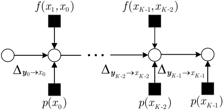
Eq. (50) shows that 𝒚k→xk→𝒚k+1\boldsymbol{y}_{k}\to x_{k}\to\boldsymbol{y}_{k+1} forms a Markov chain. Thus, the related messages passing reduced to forward and backward recursions. The forward message recursion calculates the messages passed from 𝒚k\boldsymbol{y}_{k} to xkx_{k}, while the backward recursion calculates the messages from 𝒚k+1\boldsymbol{y}_{k+1} to xkx_{k}, ∀k\forall k. The detailed message passing process is described below.

IV-A1 Forward message recursion

The message from 𝒚k\boldsymbol{y}_{k} to xkx_{k} is

Δ𝒚k→xk​(xk)\displaystyle\Delta_{\boldsymbol{y}_{k}\rightarrow x_{k}}(x_{k}) ∝∑xk−1,𝒄p⁡(𝒚k|xk,xk−1,𝒄)​Δxk−1→𝒚k​(xk−1)​∏b=1BΔcb→𝒚k​(cb)\displaystyle\varpropto\sum_{x_{k-1},\boldsymbol{c}}p(\boldsymbol{y}_{k}|x_{k},x_{k-1},\boldsymbol{c})\Delta_{x_{k-1}\rightarrow\boldsymbol{y}_{k}}(x_{k-1})\prod_{b=1}^{B}\Delta_{c_{b}\rightarrow\boldsymbol{y}_{k}}(c_{b})
≈∑xk−1∫𝝃k,𝝃~k𝒞​𝒩​(𝒚k,xk​𝝃k+xk−1​𝝃~k,σ2​𝐈M)​Δxk−1→𝒚k​(xk−1)\displaystyle\approx\sum_{x_{k-1}}\int_{\boldsymbol{\xi}_{k},\tilde{\boldsymbol{\xi}}_{k}}\mathcal{CN}(\boldsymbol{y}_{k};x_{k}\boldsymbol{\xi}_{k}\!+\!x_{k-1}\tilde{\boldsymbol{\xi}}_{k},\sigma^{2}\mathbf{I}_{M})\Delta_{x_{k-1}\rightarrow\boldsymbol{y}_{k}}(x_{k-1})
∏m=1M𝒞​𝒩​(ξk,m,μξk,m,νξk,m)​𝒞​𝒩​(ξ~k,m,μξ~k,m,νξ~k,m),∀k,\displaystyle~~\prod_{m=1}^{M}\mathcal{CN}(\xi_{k,m};\mu_{\xi_{k,m}},\nu_{\xi_{k,m}})\mathcal{CN}(\tilde{\xi}_{k,m};\mu_{\tilde{\xi}_{k,m}},\nu_{\tilde{\xi}_{k,m}}),\forall k, (51)

where (51) is based on the fact that 𝒄→(𝝃k,𝝃~k)→𝒚k\boldsymbol{c}\to(\boldsymbol{\xi}_{k},\tilde{\boldsymbol{\xi}}_{k})\to\boldsymbol{y}_{k} forms a Markov chain and the approximation that {ξk,m}\{\xi_{k,m}\} and {ξ~k,m}\{\tilde{\xi}_{k,m}\} are independent of each other. With the message from 𝒄\boldsymbol{c}, i.e., ∏b=1BΔcb→𝒚k​(cb)\prod_{b=1}^{B}\Delta_{c_{b}\rightarrow\boldsymbol{y}_{k}}(c_{b}), we have μξk,m=hk,mUB+∑n=1Nhk,m,n​θn​s^n\mu_{\xi_{k,m}}=h_{k,m}^{\rm UB}+\sum_{n=1}^{N}h_{k,m,n}\theta_{n}\hat{s}_{n}, νξk,m=∑n=1Nhk,m,n2​νsn\nu_{\xi_{k,m}}=\sum_{n=1}^{N}h_{k,m,n}^{2}\nu_{s_{n}}, μξ~k,m=∑n=1Nh~k,m,n​θn​(1−s^n)\mu_{\tilde{\xi}_{k,m}}=\sum_{n=1}^{N}\tilde{h}_{k,m,n}\theta_{n}(1-\hat{s}_{n}), and νξ~k,m=∑n=1Nh~k,m,n2​νsn\nu_{\tilde{\xi}_{k,m}}=\sum_{n=1}^{N}\tilde{h}_{k,m,n}^{2}\nu_{s_{n}}, ∀k,m\forall k,m, where s^n=c^b\hat{s}_{n}=\hat{c}_{b}, νsn=νcb\nu_{s_{n}}=\nu_{c_{b}} if ⌈nL⌉=b\lceil\frac{n}{L}\rceil=b, ∀n\forall n, and ({c^b},{νcb})(\{\hat{c}_{b}\},\{\nu_{c_{b}}\}) are respectively the estimated means and variances of {cb}\{c_{b}\} in the last iteration. Δxk−1→𝒚k​(xk−1)\Delta_{x_{k-1}\rightarrow\boldsymbol{y}_{k}}(x_{k-1}) in (51) is the message from xk−1x_{k-1} to 𝒚k\boldsymbol{y}_{k}, given by

Δxk−1→𝒚k​(xk−1)∝p⁡(xk−1)​Δ𝒚k−1→xk−1​(xk−1),∀k,\displaystyle\Delta_{x_{k-1}\rightarrow\boldsymbol{y}_{k}}(x_{k-1})\varpropto p(x_{k-1})\Delta_{\boldsymbol{y}_{k-1}\rightarrow x_{k-1}}(x_{k-1}),\forall k, (52)

where Δ𝒚0→x0​(x0)≜1\Delta_{\boldsymbol{y}_{0}\rightarrow x_{0}}(x_{0})\triangleq 1.

Eq. (51) involves integration over all the 2​M2M variables in 𝝃k\boldsymbol{\xi}_{k} and 𝝃~k\tilde{\boldsymbol{\xi}}_{k}. To reduce the computational complexity, we apply the MRC technique to 𝒚k\boldsymbol{y}_{k} as

𝝁𝝃kH​𝒚k‖𝝁𝝃k‖2\displaystyle\frac{\boldsymbol{\mu}_{\boldsymbol{\xi}_{k}}^{\rm H}\boldsymbol{y}_{k}}{\|\boldsymbol{\mu}_{\boldsymbol{\xi}_{k}}\|^{2}} =xk​𝝁𝝃kH​𝝃k‖𝝁𝝃k‖2+xk−1​𝝁𝝃kH​𝝃~k‖𝝁𝝃k‖2+𝝁𝝃kH​𝒘k‖𝝁𝝃k‖2,\displaystyle=x_{k}\frac{\boldsymbol{\mu}_{\boldsymbol{\xi}_{k}}^{\rm H}\boldsymbol{\xi}_{k}}{\|\boldsymbol{\mu}_{\boldsymbol{\xi}_{k}}\|^{2}}+x_{k-1}\frac{\boldsymbol{\mu}_{\boldsymbol{\xi}_{k}}^{\rm H}\tilde{\boldsymbol{\xi}}_{k}}{\|\boldsymbol{\mu}_{\boldsymbol{\xi}_{k}}\|^{2}}+\frac{\boldsymbol{\mu}_{\boldsymbol{\xi}_{k}}^{\rm H}\boldsymbol{w}_{k}}{\|\boldsymbol{\mu}_{\boldsymbol{\xi}_{k}}\|^{2}}, (53)

where 𝝁𝝃k=[μξk,1,⋯,μξk,M]T\boldsymbol{\mu}_{\boldsymbol{\xi}_{k}}=[\mu_{\xi_{k,1}},\cdots,\mu_{\xi_{k,M}}]^{\rm T}. Denote by ykF=𝝁𝝃kH​𝒚k‖𝝁𝝃k‖2y_{k}^{\rm F}=\frac{\boldsymbol{\mu}_{\boldsymbol{\xi}_{k}}^{\rm H}\boldsymbol{y}_{k}}{\|\boldsymbol{\mu}_{\boldsymbol{\xi}_{k}}\|^{2}}, hkF=𝝁𝝃kH​𝝃k‖𝝁𝝃k‖2∼𝒞​𝒩​(⋅,μhkF,νhkF)h_{k}^{\rm F}=\frac{\boldsymbol{\mu}_{\boldsymbol{\xi}_{k}}^{\rm H}\boldsymbol{\xi}_{k}}{\|\boldsymbol{\mu}_{\boldsymbol{\xi}_{k}}\|^{2}}\sim\mathcal{CN}\left(\cdot;\mu_{h_{k}^{\rm F}},\nu_{h_{k}^{\rm F}}\right), where μhkF=1\mu_{h_{k}^{\rm F}}=1 and νhkF=∑m=1Mμξk,m2​νξk,m(‖𝝁𝝃k‖2)2\nu_{h_{k}^{\rm F}}=\frac{\sum_{m=1}^{M}\mu_{\xi_{k,m}}^{2}\nu_{\xi_{k,m}}}{(\|\boldsymbol{\mu}_{\boldsymbol{\xi}_{k}}\|^{2})^{2}}, h~kF=𝝁𝝃kH​𝝃~k‖𝝁𝝃k‖2∼𝒞​𝒩​(⋅,μh~kF,νh~kF)\tilde{h}_{k}^{\rm F}=\frac{\boldsymbol{\mu}_{\boldsymbol{\xi}_{k}}^{\rm H}\tilde{\boldsymbol{\xi}}_{k}}{\|\boldsymbol{\mu}_{\boldsymbol{\xi}_{k}}\|^{2}}\sim\mathcal{CN}\left(\cdot;\mu_{\tilde{h}_{k}^{\rm F}},\nu_{\tilde{h}_{k}^{\rm F}}\right), where μh~kF=𝝁𝝃kH​𝝁𝝃~k‖𝝁𝝃k‖2\mu_{\tilde{h}_{k}^{\rm F}}=\frac{\boldsymbol{\mu}_{\boldsymbol{\xi}_{k}}^{\rm H}\boldsymbol{\mu}_{\tilde{\boldsymbol{\xi}}_{k}}}{\|\boldsymbol{\mu}_{\boldsymbol{\xi}_{k}}\|^{2}} and νh~kF=∑m=1Mμξk,m2​νξ~k,m(‖𝝁𝝃k‖2)2\nu_{\tilde{h}_{k}^{\rm F}}=\frac{\sum_{m=1}^{M}\mu_{\xi_{k,m}}^{2}\nu_{\tilde{\xi}_{k,m}}}{(\|\boldsymbol{\mu}_{\boldsymbol{\xi}_{k}}\|^{2})^{2}}, and 𝝁𝝃kH​𝒘k‖𝝁𝝃k‖2∼𝒞​𝒩​(⋅,0,σ2)\frac{\boldsymbol{\mu}_{\boldsymbol{\xi}_{k}}^{\rm H}\boldsymbol{w}_{k}}{\|\boldsymbol{\mu}_{\boldsymbol{\xi}_{k}}\|^{2}}\sim\mathcal{CN}(\cdot;0,\sigma^{2}). Then, (51) is simplified to

Δ𝒚k→xk​(xk)\displaystyle\Delta_{\boldsymbol{y}_{k}\rightarrow x_{k}}(x_{k})
∝∑xk−1∫hkF,h~kF𝒞​𝒩​(ykF,xk​hkF+xk−1​h~kF,σ2)​Δxk−1→𝒚k​(xk−1)​𝒞​𝒩​(hkF,1,νhkF)​𝒞​𝒩​(h~kF,μh~kF,νh~kF)\displaystyle\varpropto\sum_{x_{k-1}}\int_{h_{k}^{\rm F},\tilde{h}_{k}^{\rm F}}\mathcal{CN}\left(y_{k}^{\rm F};x_{k}h_{k}^{\rm F}+x_{k-1}\tilde{h}_{k}^{\rm F},\sigma^{2}\right)\Delta_{x_{k-1}\rightarrow\boldsymbol{y}_{k}}(x_{k-1})\mathcal{CN}(h_{k}^{\rm F};1,\nu_{h_{k}^{\rm F}})\mathcal{CN}(\tilde{h}_{k}^{\rm F};\mu_{\tilde{h}_{k}^{\rm F}},\nu_{\tilde{h}_{k}^{\rm F}})
=∑xk−1p⁡(xk−1)​Δ𝒚k−1→xk−1​(xk−1)​𝒞​𝒩​(ykF,xk+xk−1​μh~kF,σ2+xk2​νhkF+xk−12​νh~kF)⏟≜f⁡(xk,xk−1),∀k.\displaystyle=\sum_{x_{k-1}}p(x_{k-1})\Delta_{\boldsymbol{y}_{k-1}\rightarrow x_{k-1}}(x_{k-1})\underbrace{\mathcal{CN}\left(y_{k}^{\rm F};x_{k}+x_{k-1}\mu_{\tilde{h}_{k}^{\rm F}},\sigma^{2}+x_{k}^{2}\nu_{h_{k}^{\rm F}}+x_{k-1}^{2}\nu_{\tilde{h}_{k}^{\rm F}}\right)}_{\triangleq f(x_{k},x_{k-1})},\forall k. (54)

(54) implies a forward message recursion over Δ𝒚k→xk​(xk),∀k\Delta_{\boldsymbol{y}_{k}\rightarrow x_{k}}(x_{k}),\forall k, which is represented by Fig. 3.

Refer to caption
Fig. 3: Forward recursion for the message computation where f⁡(xk,xk−1)f(x_{k},x_{k-1}) is defined in eq. (54).
Fig. 4: Backward recursion for the message computation where b⁡(xk,xk−1)b(x_{k},x_{k-1}) is defined in eq. (58).

IV-A2 Backward message recursion

The message from 𝒚k\boldsymbol{y}_{k} to xk−1x_{k-1} is

Δ𝒚k→xk−1​(xk−1)∝∑xk,𝒄p⁡(𝒚k|xk,xk−1,𝒄)​Δxk→𝒚k​(xk)​∏b=1BΔcb→𝒚k​(cb),∀k,\displaystyle\Delta_{\boldsymbol{y}_{k}\rightarrow x_{k-1}}(x_{k-1})\varpropto\sum_{x_{k},\boldsymbol{c}}p(\boldsymbol{y}_{k}|x_{k},x_{k-1},\boldsymbol{c})\Delta_{x_{k}\rightarrow\boldsymbol{y}_{k}}(x_{k})\prod_{b=1}^{B}\Delta_{c_{b}\rightarrow\boldsymbol{y}_{k}}(c_{b}),\forall k, (55)

where Δxk→𝒚k​(xk)\Delta_{x_{k}\rightarrow\boldsymbol{y}_{k}}(x_{k}) is the message from xkx_{k} to 𝒚k\boldsymbol{y}_{k} given as

Δxk→𝒚k​(xk)∝p⁡(xk)​Δ𝒚k+1→xk​(xk),∀k,\displaystyle\Delta_{x_{k}\rightarrow\boldsymbol{y}_{k}}(x_{k})\varpropto p(x_{k})\Delta_{\boldsymbol{y}_{k+1}\rightarrow x_{k}}(x_{k}),\forall k, (56)

with Δ𝒚K+1→xK​(xK)≜1\Delta_{\boldsymbol{y}_{K+1}\rightarrow x_{K}}(x_{K})\triangleq 1.

Similar to the forward message recursion, we apply the backward MRC to 𝒚k\boldsymbol{y}_{k} for ease the computation of (55). The backward MRC is designed as

𝝁𝝃~kH​𝒚k‖𝝁𝝃~k‖2\displaystyle\frac{\boldsymbol{\mu}_{\tilde{\boldsymbol{\xi}}_{k}}^{\rm H}\boldsymbol{y}_{k}}{\|\boldsymbol{\mu}_{\tilde{\boldsymbol{\xi}}_{k}}\|^{2}} =xk​𝝁𝝃~kH​𝝃k‖𝝁𝝃~k‖2+xk−1​𝝁𝝃~kH​𝝃~k‖𝝁𝝃~k‖2+𝝁𝝃~kH​𝒘k‖𝝁𝝃~k‖2,\displaystyle=x_{k}\frac{\boldsymbol{\mu}_{\tilde{\boldsymbol{\xi}}_{k}}^{\rm H}\boldsymbol{\xi}_{k}}{\|\boldsymbol{\mu}_{\tilde{\boldsymbol{\xi}}_{k}}\|^{2}}+x_{k-1}\frac{\boldsymbol{\mu}_{\tilde{\boldsymbol{\xi}}_{k}}^{\rm H}\tilde{\boldsymbol{\xi}}_{k}}{\|\boldsymbol{\mu}_{\tilde{\boldsymbol{\xi}}_{k}}\|^{2}}+\frac{\boldsymbol{\mu}_{\tilde{\boldsymbol{\xi}}_{k}}^{\rm H}\boldsymbol{w}_{k}}{\|\boldsymbol{\mu}_{\tilde{\boldsymbol{\xi}}_{k}}\|^{2}}, (57)

where 𝝁𝝃~k=[μξ~k,1,⋯,μξ~k,M]T\boldsymbol{\mu}_{\tilde{\boldsymbol{\xi}}_{k}}=[\mu_{\tilde{\xi}_{k,1}},\cdots,\mu_{\tilde{\xi}_{k,M}}]^{\rm T}. Denote by ykB=𝝁𝝃~kH​𝒚k‖𝝁𝝃~k‖2y_{k}^{\rm B}=\frac{\boldsymbol{\mu}_{\tilde{\boldsymbol{\xi}}_{k}}^{\rm H}\boldsymbol{y}_{k}}{\|\boldsymbol{\mu}_{\tilde{\boldsymbol{\xi}}_{k}}\|^{2}}, hkB=𝝁𝝃~kH​𝝃k‖𝝁𝝃~k‖2∼𝒞​𝒩​(⋅,μhkB,νhkB)h_{k}^{\rm B}=\frac{\boldsymbol{\mu}_{\tilde{\boldsymbol{\xi}}_{k}}^{\rm H}\boldsymbol{\xi}_{k}}{\|\boldsymbol{\mu}_{\tilde{\boldsymbol{\xi}}_{k}}\|^{2}}\sim\mathcal{CN}\left(\cdot;\mu_{h_{k}^{\rm B}},\nu_{h_{k}^{\rm B}}\right), where μhkB=𝝁𝝃~kH​𝝁𝝃k‖𝝁𝝃~k‖2\mu_{h_{k}^{\rm B}}=\frac{\boldsymbol{\mu}_{\tilde{\boldsymbol{\xi}}_{k}}^{\rm H}\boldsymbol{\mu}_{\boldsymbol{\xi}_{k}}}{\|\boldsymbol{\mu}_{\tilde{\boldsymbol{\xi}}_{k}}\|^{2}} and νhkB=∑m=1Mμξ~k,m2​νξk,m(‖𝝁𝝃~k‖2)2\nu_{h_{k}^{\rm B}}=\frac{\sum_{m=1}^{M}\mu_{\tilde{\xi}_{k,m}}^{2}\nu_{\xi_{k,m}}}{(\|\boldsymbol{\mu}_{\tilde{\boldsymbol{\xi}}_{k}}\|^{2})^{2}}, h~kB=𝝁𝝃~kH​𝝃~k‖𝝁𝝃~k‖2∼𝒞​𝒩​(⋅,μh~kB,νh~kB)\tilde{h}_{k}^{\rm B}=\frac{\boldsymbol{\mu}_{\tilde{\boldsymbol{\xi}}_{k}}^{\rm H}\tilde{\boldsymbol{\xi}}_{k}}{\|\boldsymbol{\mu}_{\tilde{\boldsymbol{\xi}}_{k}}\|^{2}}\sim\mathcal{CN}\left(\cdot;\mu_{\tilde{h}_{k}^{\rm B}},\nu_{\tilde{h}_{k}^{\rm B}}\right), where μh~kB=1\mu_{\tilde{h}_{k}^{\rm B}}=1 and νh~kB=∑m=1Mμξ~k,m2​νξ~k,m(‖𝝁𝝃~k‖2)2\nu_{\tilde{h}_{k}^{\rm B}}=\frac{\sum_{m=1}^{M}\mu_{\tilde{\xi}_{k,m}}^{2}\nu_{\tilde{\xi}_{k,m}}}{(\|\boldsymbol{\mu}_{\tilde{\boldsymbol{\xi}}_{k}}\|^{2})^{2}}, and 𝝁𝝃~kH​𝒘k‖𝝁𝝃~k‖2∼𝒞​𝒩​(⋅,0,σ2)\frac{\boldsymbol{\mu}_{\tilde{\boldsymbol{\xi}}_{k}}^{\rm H}\boldsymbol{w}_{k}}{\|\boldsymbol{\mu}_{\tilde{\boldsymbol{\xi}}_{k}}\|^{2}}\sim\mathcal{CN}(\cdot;0,\sigma^{2}). Then, (55) is simplified to

Δ𝒚k→xk−1​(xk−1)\displaystyle\Delta_{\boldsymbol{y}_{k}\rightarrow x_{k-1}}(x_{k-1})
∝∑xkp⁡(xk)​Δ𝒚k+1→xk​(xK)​𝒞​𝒩​(ykB,xk​μhkB+xk−1,σ2+xk2​νhkB+xk−12​νh~kB)⏟≜b⁡(xk,xk−1),∀k.\displaystyle\varpropto\sum_{x_{k}}p(x_{k})\Delta_{\boldsymbol{y}_{k+1}\rightarrow x_{k}}(x_{K})\underbrace{\mathcal{CN}\left(y_{k}^{\rm B};x_{k}\mu_{h_{k}^{\rm B}}+x_{k-1},\sigma^{2}+x_{k}^{2}\nu_{h_{k}^{\rm B}}+x_{k-1}^{2}\nu_{\tilde{h}_{k}^{\rm B}}\right)}_{\triangleq b(x_{k},x_{k-1})},\forall k. (58)

The backward message recursion over Δ𝒚k→xk−1​(xk−1),∀k\Delta_{\boldsymbol{y}_{k}\rightarrow x_{k-1}}(x_{k-1}),\forall k in (58) is represented by Fig. 4. The estimated mean and variance of xkx_{k} are respectively computed as

x^k\displaystyle\hat{x}_{k} =∑xkxk​p​(xk)​Δ𝒚k→xk​(xk)​Δ𝒚k+1→xk​(xk),\displaystyle=\sum_{x_{k}}x_{k}p(x_{k})\Delta_{\boldsymbol{y}_{k}\rightarrow x_{k}}(x_{k})\Delta_{\boldsymbol{y}_{k+1}\rightarrow x_{k}}(x_{k}), (59)
νxk\displaystyle\nu_{x_{k}} =∑xk|xk−x^k|2​p​(xk)​Δ𝒚k→xk​(xk)​Δ𝒚k+1→xk​(xk),∀k.\displaystyle=\sum_{x_{k}}|x_{k}-\hat{x}_{k}|^{2}p(x_{k})\Delta_{\boldsymbol{y}_{k}\rightarrow x_{k}}(x_{k})\Delta_{\boldsymbol{y}_{k+1}\rightarrow x_{k}}(x_{k}),\forall k. (60)

IV-B Message Passing for Detecting 𝐜\boldsymbol{c}

The detection of 𝒄\boldsymbol{c} is carried out by message passing over the lower part of Fig. 2. First, we calculate the message passed from its upper part. For computational convenience, each xkx_{k} is approximated as a Gaussian variable with probability 𝒞𝒩(;x^k,νxk)\mathcal{CN}(;\hat{x}_{k},\nu_{x_{k}}), ∀k∈ℐk−1\forall k\in\mathcal{I}_{k-1} during the lower part message passing process. The residual of xkx_{k} is defined as xk−x^k∼𝒞𝒩(;0,νxk)x_{k}-\hat{x}_{k}\sim\mathcal{CN}(;0,\nu_{x_{k}}). To proceed, we recast (8) as

𝒚k−x^k​𝒉kUB−x^k​𝑯~k​𝜽\displaystyle\boldsymbol{y}_{k}-\hat{x}_{k}\boldsymbol{h}_{k}^{\rm UB}-\hat{x}_{k}\tilde{\boldsymbol{H}}_{k}\boldsymbol{\theta} =x^k​(𝑯k−𝑯~k)​𝚯​𝑻​𝒄+𝒏k,∀k,\displaystyle=\hat{x}_{k}(\boldsymbol{H}_{k}-\tilde{\boldsymbol{H}}_{k})\boldsymbol{\Theta}\boldsymbol{T}\boldsymbol{c}+\boldsymbol{n}_{k},\forall k, (61)

where 𝒏k\boldsymbol{n}_{k} is the equivalent noise for detecting 𝒄\boldsymbol{c}, defined as

𝒏k=(xk−x^k)​((𝑯k−𝑯~k)​𝚯​𝑻​𝒄+𝒉kUB+𝑯~k​𝜽)+𝒘k,∀k.\displaystyle\boldsymbol{n}_{k}=(x_{k}-\hat{x}_{k})\left((\boldsymbol{H}_{k}-\tilde{\boldsymbol{H}}_{k})\boldsymbol{\Theta}\boldsymbol{T}\boldsymbol{c}+\boldsymbol{h}_{k}^{\rm UB}+\tilde{\boldsymbol{H}}_{k}\boldsymbol{\theta}\right)+\boldsymbol{w}_{k},\forall k. (62)

Eq. (61) provides an explicit linear model for the estimation of 𝒄\boldsymbol{c} with observations {𝒚k−x^k​𝒉kUB−x^k​𝑯~k​𝜽}\{\boldsymbol{y}_{k}-\hat{x}_{k}\boldsymbol{h}_{k}^{\rm UB}-\hat{x}_{k}\tilde{\boldsymbol{H}}_{k}\boldsymbol{\theta}\} and measurements {x^k​(𝑯k−𝑯~k)​𝚯​𝑻}\{\hat{x}_{k}(\boldsymbol{H}_{k}-\tilde{\boldsymbol{H}}_{k})\boldsymbol{\Theta}\boldsymbol{T}\}. An existing message passing algorithm to handle this model is the GAMP [26], which is used here to recover 𝒄\boldsymbol{c}. The details of the GAMP algorithm is omitted here for brevity.

IV-C Algorithm Summary

Algorithm 4 ​: The BMP algorithm
0:  𝒚\boldsymbol{y}, {𝒉kUB}\{\boldsymbol{h}_{k}^{\rm UB}\}, {𝑯k}\{\boldsymbol{H}_{k}\}, {𝑯~k}\{\tilde{\boldsymbol{H}}_{k}\}, 𝒳\mathcal{X} Initialization: c^b=12\hat{c}_{b}=\frac{1}{2}, νcb=14\nu_{c_{b}}=\frac{1}{4}, ∀b\forall b repeat
1:    ∀k,m:\forall k,m: μξk,m=hk,mUB+∑n=1Nhk,m,n​θn​s^n\mu_{\xi_{k,m}}=h_{k,m}^{\rm UB}+\sum_{n=1}^{N}h_{k,m,n}\theta_{n}\hat{s}_{n}, νξk,m=∑n=1Nhk,m,n2​νsn\nu_{\xi_{k,m}}=\sum_{n=1}^{N}h_{k,m,n}^{2}\nu_{s_{n}}      μξ~k,m=∑n=1Nh~k,m,n​θn​(1−s^n)\mu_{\tilde{\xi}_{k,m}}=\sum_{n=1}^{N}\tilde{h}_{k,m,n}\theta_{n}(1-\hat{s}_{n}), νξ~k,m=∑n=1Nh~k,m,n2​νsn\nu_{\tilde{\xi}_{k,m}}=\sum_{n=1}^{N}\tilde{h}_{k,m,n}^{2}\nu_{s_{n}}
2:    ∀k:\forall k: μhkF=1\mu_{h_{k}^{\rm F}}=1, νhkF=∑m=1Mμξk,m2​νξk,m(‖𝝁𝝃k‖2)2\nu_{h_{k}^{\rm F}}=\frac{\sum_{m=1}^{M}\mu_{\xi_{k,m}}^{2}\nu_{\xi_{k,m}}}{(\|\boldsymbol{\mu}_{\boldsymbol{\xi}_{k}}\|^{2})^{2}}, μh~kF=𝝁𝝃kH​𝝁𝝃~k‖𝝁𝝃k‖2\mu_{\tilde{h}_{k}^{\rm F}}=\frac{\boldsymbol{\mu}_{\boldsymbol{\xi}_{k}}^{\rm H}\boldsymbol{\mu}_{\tilde{\boldsymbol{\xi}}_{k}}}{\|\boldsymbol{\mu}_{\boldsymbol{\xi}_{k}}\|^{2}}, νh~kF=∑m=1Mμξk,m2​νξ~k,m(‖𝝁𝝃k‖2)2\nu_{\tilde{h}_{k}^{\rm F}}=\frac{\sum_{m=1}^{M}\mu_{\xi_{k,m}}^{2}\nu_{\tilde{\xi}_{k,m}}}{(\|\boldsymbol{\mu}_{\boldsymbol{\xi}_{k}}\|^{2})^{2}}     μhkB=𝝁𝝃~kH​𝝁𝝃k‖𝝁𝝃~k‖2\mu_{h_{k}^{\rm B}}=\frac{\boldsymbol{\mu}_{\tilde{\boldsymbol{\xi}}_{k}}^{\rm H}\boldsymbol{\mu}_{\boldsymbol{\xi}_{k}}}{\|\boldsymbol{\mu}_{\tilde{\boldsymbol{\xi}}_{k}}\|^{2}}, νhkB=∑m=1Mμξ~k,m2​νξk,m(‖𝝁𝝃~k‖2)2\nu_{h_{k}^{\rm B}}=\frac{\sum_{m=1}^{M}\mu_{\tilde{\xi}_{k,m}}^{2}\nu_{\xi_{k,m}}}{(\|\boldsymbol{\mu}_{\tilde{\boldsymbol{\xi}}_{k}}\|^{2})^{2}}, μh~kB=1\mu_{\tilde{h}_{k}^{\rm B}}=1, νh~kB=∑m=1Mμξ~k,m2​νξ~k,m(‖𝝁𝝃~k‖2)2\nu_{\tilde{h}_{k}^{\rm B}}=\frac{\sum_{m=1}^{M}\mu_{\tilde{\xi}_{k,m}}^{2}\nu_{\tilde{\xi}_{k,m}}}{(\|\boldsymbol{\mu}_{\tilde{\boldsymbol{\xi}}_{k}}\|^{2})^{2}}   for k=1,2,…,K−1k=1,2,\ldots,K-1  % Forward recursion
3:      Δ𝒚k→xk​(xk)∝∑xk−1p⁡(xk−1)​Δ𝒚k−1→xk−1​(xk−1)​f​(xk,xk−1)\Delta_{\boldsymbol{y}_{k}\rightarrow x_{k}}(x_{k})\varpropto\sum_{x_{k-1}}p(x_{k-1})\Delta_{\boldsymbol{y}_{k-1}\rightarrow x_{k-1}}(x_{k-1})f(x_{k},x_{k-1})   end for  for k=K,K−1,…,2k=K,K-1,\ldots,2  % Backward recursion
4:      Δ𝒚k→xk−1​(xk−1)∝∑xkp⁡(xk)​Δ𝒚k+1→xk​(xk)​b​(xk,xk−1)\Delta_{\boldsymbol{y}_{k}\rightarrow x_{k-1}}(x_{k-1})\varpropto\sum_{x_{k}}p(x_{k})\Delta_{\boldsymbol{y}_{k+1}\rightarrow x_{k}}(x_{k})b(x_{k},x_{k-1})   end for
5:    ∀k:\forall k: x^k=∑xkxk​p​(xk)​Δ𝒚k→xk​(xk)​Δ𝒚k+1→xk​(xk)\hat{x}_{k}=\sum_{x_{k}}x_{k}p(x_{k})\Delta_{\boldsymbol{y}_{k}\rightarrow x_{k}}(x_{k})\Delta_{\boldsymbol{y}_{k+1}\rightarrow x_{k}}(x_{k})     νxk=∑xk|xk−x^k|2​p​(xk)​Δ𝒚k→xk​(xk)​Δ𝒚k+1→xk​(xk)\nu_{x_{k}}=\sum_{x_{k}}|x_{k}-\hat{x}_{k}|^{2}p(x_{k})\Delta_{\boldsymbol{y}_{k}\rightarrow x_{k}}(x_{k})\Delta_{\boldsymbol{y}_{k+1}\rightarrow x_{k}}(x_{k})
6:    ∀k:\forall k: Detecting 𝒄\boldsymbol{c} based on the linear model given in eq. (61) by GAMP algorithm.until a certain stopping criterion is met
6:  {x^k}\{\hat{x}_{k}\} and {c^b}\{\hat{c}_{b}\}.

The overall BMP algorithm is summarized in Algorithm 4. In specific, Line 11 updates the means and variances of the auxiliary variables {ξk,m}\{\xi_{k,m}\} and {ξ~k,m}\{\tilde{\xi}_{k,m}\}. Line 22 updates the means and variances of the auxiliary variables {hkF}\{h_{k}^{\rm F}\}, {h~kF}\{\tilde{h}_{k}^{\rm F}\}, {hkB}\{h_{k}^{\rm B}\}, and {h~kB}\{\tilde{h}_{k}^{\rm B}\}. Line 33 recursively computes the messages from {𝒚k}\{\boldsymbol{y}_{k}\} to {xk}\{x_{k}\}, where Δ𝒚0→x0​(x0)=1\Delta_{\boldsymbol{y}_{0}\rightarrow x_{0}}(x_{0})=1 and p⁡(x0)=δ⁡(0)p(x_{0})=\delta(0). Line 44 recursively computes the messages from {𝒚k}\{\boldsymbol{y}_{k}\} to {xk−1}\{x_{k-1}\}, where Δ𝒚K+1→xK​(xK)=1\Delta_{\boldsymbol{y}_{K+1}\rightarrow x_{K}}(x_{K})=1 and p⁡(xk)=δ⁡(0)p(x_{k})=\delta(0). Line 55 updates of the estimated means {x^k}\{\hat{x}_{k}\} and variances {νxk}\{\nu_{{x}_{k}}\} for {xk}\{x_{k}\}. Line 66 performs the GAMP algorithm to detect 𝒄\boldsymbol{c}. The stopping criterion is defined as 𝔼​||yk,m−x^k​μξk,m−x^k−1​μξ~k,m|2−σ2|≤ϵ\mathbbmss{E}\left|\left|y_{k,m}-\hat{x}_{k}\mu_{\xi_{k,m}}\!-\!\hat{x}_{k-1}\mu_{\tilde{\xi}_{k,m}}\right|^{2}-\sigma^{2}\right|\leq\epsilon, where ϵ\epsilon is the tolerance parameter, or is when the iteration number reaching to the preset maximum value.

We now analyze the computational complexity of the proposed BMP algorithm. The complexity in Line 11 is 𝒪⁡(K​M​N)\mathcal{O}(KMN). The complexity in Line 22 is 𝒪⁡(K​M)\mathcal{O}(KM). The complexities in Line 33 and Line 44 are both 𝒪⁡(|𝒳|2)\mathcal{O}(|\mathcal{X}|^{2}), and thus the complexities of the “for” loops therein are 𝒪⁡(K​|𝒳|2)\mathcal{O}(K|\mathcal{X}|^{2}). The complexity in Line 55 is 𝒪⁡(K​|𝒳|)\mathcal{O}(K|\mathcal{X}|). The complexity in Line 66 depends on the complexity of the GAMP algorithm, which is 𝒪⁡(K​M​B)\mathcal{O}(KMB) [26].

V Numerical Results

This section conducts numerical experiments to evaluate the performance of the proposed FRM-OFDM scheme for RIS-aided transmission, the AO and RAO algorithms for the system optimization, and the BMP algorithm for the bilinear signal detection. First, we describe the simulation setup.

V-A Simulation Setup

Refer to caption
Fig. 5: The simulated RIS-aided FRM-OFDM scenario.

We consider a three-dimensional (3D) Cartesian coordinate system shown in Fig. 5. The BS is placed at (0,0,50)(0;0;50), the user is located at (50,0,0)(50;0;0), and the RIS is randomly deployed at (50​ς,30,50)(50\varsigma;30;50) with ς\varsigma is a random number between [0,1][0,1]. The multipath numbers of the user-BS, user-RIS, and RIS-BS links are set to 88, 88, and 66, respectively. The CP length is selected to perfectly suppress the ISI. Usually, the deployment location of the RIS is chosen to favor line-of-sight (LoS) transmission between the RIS and the BS/user. Thus, the first paths of the user-RIS and RIS-BS links are modeled as LoS paths, and the remaining paths are treated as non-LoS (NLoS) paths characterized by Rayleigh fading. For the user-BS link, the LoS path is assumed to be blocked by obstacles, with only NLoS paths. The entries of the NLoS paths are independently taken from the CSCG distribution 𝒞​𝒩​(0,1)\mathcal{CN}(0,1). Since the size of the RIS array is practically much smaller than the distance between the RIS and the BS/user, a far-field scenario is adopted. The RIS is assumed to be equipped with a two-dimensional (22D) uniform rectangular array, with dimension Lx×LyL_{x}\times L_{y}, where Lx=8L_{x}=8 and Ly=N8L_{y}=\frac{N}{8}. Then, the LoS path can be expressed as the 22D array steering vector, given by

𝐚⁡(ϑ,ψ)\displaystyle\mathbf{a}(\vartheta,\psi) =𝐚az​(ϑ,ψ)⊗𝐚el​(ϑ,ψ),\displaystyle=\mathbf{a}_{\textsf{az}}(\vartheta,\psi)\otimes\mathbf{a}_{\textsf{el}}(\vartheta,\psi), (63)

where ϑ\vartheta is the azimuth angle, and ψ\psi is the elevation angle. 𝐚az​(ϑ,ψ)∈ℂLx×1\mathbf{a}_{\textsf{az}}(\vartheta,\psi)\in\mathbb{C}^{L_{x}\times 1} and 𝐚el​(ϑ,ψ)∈ℂLy×1\mathbf{a}_{\textsf{el}}(\vartheta,\psi)\in\mathbb{C}^{L_{y}\times 1} are the uniform linear array (ULA) steering vectors given as

[𝐚az​(ϑ,ψ)]n\displaystyle\hskip-5.69046pt\left[\mathbf{a}_{\textsf{az}}(\vartheta,\psi)\right]_{n} =e−j​2​π​dx​(n−1)ϱ​cos⁡(ϑ)​sin⁡(ψ),∀n∈ℐLx,\displaystyle=e^{-j\frac{2\pi d_{x}(n-1)}{\varrho}\cos(\vartheta)\sin(\psi)},\forall n\in\mathcal{I}_{L_{x}}, (64)
[𝐚el​(ϑ,ψ)]n\displaystyle\left[\mathbf{a}_{\textsf{el}}(\vartheta,\psi)\right]_{n} =ej​2​π​dy​(n−1)ϱ​sin⁡(ϑ)​sin⁡(ψ),∀n∈ℐLy,\displaystyle=e^{j\frac{2\pi d_{y}(n-1)}{\varrho}\sin(\vartheta)\sin(\psi)},\forall n\in\mathcal{I}_{L_{y}}, (65)

where the wavelength of propagation ϱ\varrho is set to 3×10⁸/fc3\times 10^{8}/f_{c} meters, with fc=915f_{c}=915 MHz being the carrier frequency, dx=dy=3×10⁷/fcd_{x}=d_{y}=3\times 10^{7}/f_{c} meters are respectively the horizontal and vertical sizes of a single RIS element. κ1=3\kappa_{1}=3 dB and κ2=10\kappa_{2}=10 dB denote the power ratios of the LoS component to the NLoS component for the user-RIS link and for the RIS-BS link, respectively. The free-space path loss model proposed in [20] is adopted for the cascaded user-RIS-BS channel, given by

P​L=Guser​GRIS​GBS​Lx​Ly​dx​dy​(3×10⁸/fc)264​π3​dUR​dRB,\displaystyle PL=G_{\rm user}G_{\rm RIS}G_{\rm BS}\frac{L_{x}L_{y}d_{x}d_{y}(3\times 10^{8}/f_{c})^{2}}{64\pi^{3}d_{\rm UR}d_{\rm RB}}, (66)

where Guser=0G_{\rm user}=0 dBi, GRIS=5G_{\rm RIS}=5 dBi, and GBS=0G_{\rm BS}=0 dBi are respectively the antenna gain at the user, the RIS, and the BS, and dRB/dURd_{\rm RB}/d_{\rm UR} is the distance between the RIS and the BS/user. The free-space path loss of the user-BS link is modeled as β=β0​d−α\beta=\beta_{0}d^{-\alpha}, where β0=−30\beta_{0}=-30 dB, dd is the link distance, and α=2.2\alpha=2.2.

In simulations, the elements of 𝑿\boldsymbol{X} are randomly taken from the quadrature phase shift keying (QPSK) modulation with Gray-mapping. The noise variance σ2\sigma^{2} is set to −60-60 dBw. The iteration numbers are set to 100100 for the MM algorithm and 200200 for the AO and RAO algorithms. The maximum iteration number is set to 1010 for the BMP algorithm. The error tolerance threshold for the BMP algorithm is set to ϵ=10−3\epsilon=10^{-3}. The presented simulation results are obtained by taking average over at least 10001000 random realizations. The unit of the rate is bit per channel use per SC (bpcu). The number of RIS blocks BB is set to its maximum, i.e., NN, in Figs. 66, 77, 88, and 99.

V-B Simulations of RIS Phase shift Optimization Design

Fig. 6: Comparison of I⁡(𝒙,𝒔,𝒚)I(\boldsymbol{x},\boldsymbol{s};\boldsymbol{y}) versus the iteration time with the AO and RAO algorithms.
Fig. 7: Rate region comparison of the ORM-OFDM scheme and the FRM-OFDM scheme with M=8M=8, K=16K=16, N=128N=128, and P=0P=0 dBw.
Fig. 8: Sum rate comparison versus the number of receiver antennas MM with K=8K=8, N=192N=192, and P=0P=0 dBw.

Fig. 6 compares the sum rate performance of the AO and RAO algorithms versus the iteration time. The parameter settings are: M=8M=8, K=16K=16, and P=0P=0 dBw. We see that for both N=64N=64 and N=128N=128, the RAO algorithm shows marginal rate performance degradation as compared to the AO algorithm. Thus, in the following figures, we only present the optimization results by the RAO algorithm for a lower computational burden.

Fig. 9: Sum rate comparison versus the number of RIS elements NN with K=8K=8, M=12M=12, and P=0P=0 dBw.

Fig. 7 compares the rate region of the proposed FRM-OFDM scheme with the existing ORM-OFDM scheme. The parameter settings are: M=8M=8, K=16K=16, N=128N=128, and P=0P=0 dBw. We see that no matter 𝜽\boldsymbol{\theta} is optimized or randomly chosen from [0,2​π][0,2\pi], the ORM-OFDM scheme covers a wider rate region than the ORM-OFDM scheme. Specially, for both the 𝜽\boldsymbol{\theta} cases, the FRM-OFDM scheme outperforms the ORM-OFDM scheme by about 1.21.2 bpcu in terms of RIS rate, i.e., I⁡(𝒔,𝒚|𝒙)I(\boldsymbol{s},\boldsymbol{y}|\boldsymbol{x}), and by about 0.50.5 bpcu in terms of user rate, i.e., I⁡(𝒙,𝒚|𝒔)I(\boldsymbol{x},\boldsymbol{y}|\boldsymbol{s}). We also see that, by optimization, both the FRM-OFDM scheme and the ORM-OFDM scheme achieve about 1.51.5 bpcu gain in user rate, but have marginal improvement on the RIS rate.

Fig. 8 compares the sum rate of the FRM-OFDM scheme with the ORM-OFDM scheme, the RIS-aided OFDM system, and the OFDM without RIS case versus the number of receive antennas MM. For comparison, we also provide the user rate I⁡(𝒙;𝒚|𝒔)I(\boldsymbol{x};\boldsymbol{y}|\boldsymbol{s}) of the FRM-OFDM system. The parameter settings are: K=8K=8, N=192N=192, and P=0P=0 dBw. We see that, before optimization, the FRM-OFDM outperforms the ORM-OFDM, the RIS-aided OFDM, and the OFDM without RIS by about 44, 88, and 99 bpcu, respectively, at M=32M=32. At the same MM setting, by optimization, the rate gains of the FRM-OFDM, the ORM-OFDM, and the RIS-aided OFDM are about 11, 11, and 33 bpcu, respectively. The user rate I⁡(𝒙;𝒚|𝒔)I(\boldsymbol{x};\boldsymbol{y}|\boldsymbol{s}) of the FRM-OFDM system tightly approaches the rate of the OFDM system for random 𝜽\boldsymbol{\theta} case, while lower than the latter by about 11 bpcu after optimization. We conjecture that this is because the FRM-OFDM system sacrifices some RIS passive beamforming capability in exchanging for RIS information transfer. Fig. 8 also shows that, the FRM-OFDM has a sharper slope in rate growth than the RIS-aided OFDM as the increase of MM, which demonstrates the multiplexing gain obtained by RIS information transfer.

Fig. 9 shows the sum rate comparison of the same systems as Fig. 8 versus the number of RIS elements NN. The parameter settings are: K=8K=8, M=12M=12, and P=0P=0 dBw. We see that before optimization, the FRM-OFDM outperforms the ORM-OFDM from about 0.30.3 bpcu to about 11 bpcu, and outperforms the RIS-aided OFDM from about 0.50.5 bpcu to about 22 bpcu, as NN ranging from 3232 to 256256. By optimization, the rate gaps between the FRM-OFDM and the ORM-OFDM, and between the FRM-OFDM and the RIS-aided OFDM are about 1.51.5 and 1.31.3 bpcu, respectively, at N=128N=128. Comparing the curves of the “OFDM without RIS” and the “FRM-OFDM”, we see that the rate gain by the assistance of an RIS can be as high as 44 bpcu when N=128N=128.

V-C Simulations of Bilinear Receiver Design

Fig. 10: Convergence behavior of the TMP algorithm with M=8M=8, K=32K=32, B=20B=20, and L=4L=4.
Fig. 11: Average BERs of 𝒙\boldsymbol{x} and 𝒄\boldsymbol{c} versus the transmitted power PP with M=8M=8, K=32K=32, B=20B=20, and L=4L=4.
Fig. 12: Average BERs of 𝒙\boldsymbol{x} and 𝒄\boldsymbol{c} versus the RIS information blocks BB with M=8M=8, K=32K=32 and L=4L=4.

The convergence behavior of the TMP algorithm is presented in Fig 10. The parameter settings are: M=8M=8, K=32K=32, B=20B=20, and L=4L=4. The “Ran-𝜽\boldsymbol{\theta}” represents the random 𝜽\boldsymbol{\theta} case and the “Opt-𝜽\boldsymbol{\theta}” represents the optimized 𝜽\boldsymbol{\theta} case. We consider P=0P=0 dBw and P=5P=5 dBw for comparison. We see that in all the considered cases, the TMP algorithm converges within 44 times of iteration.

Fig. 11 shows the average bit error rate (BER) performance of the BMP algorithm versus the transmitted power PP. We consider the “FRM” (the FRM-OFDM system with random 𝜽\boldsymbol{\theta}), the “Opt-ORM” (the ORM-OFDM system with optimized 𝜽\boldsymbol{\theta}), the “Opt-FRM” (the FRM-OFDM system with optimized 𝜽\boldsymbol{\theta}), and the lower bound (LB) (which is obtained by retrieving 𝒙\boldsymbol{x} (or 𝒄\boldsymbol{c}) with perfectly known 𝒄\boldsymbol{c} (or 𝒙\boldsymbol{x}) in the FRM-OFDM system). The parameter settings are: M=8M=8, K=32K=32 and B=20B=20 and L=4L=4. We see that the FRM-OFDM tightly approaches the lower bound when detecting both 𝒙\boldsymbol{x} and 𝒄\boldsymbol{c}. When detecting 𝒙\boldsymbol{x}, the Opt-FRM outperforms the Opt-ORM by about 33 dBw, and outperforms the FRM by about 1010 dBw at the average BER of 𝒙=10−4\boldsymbol{x}=10^{-4}. The average BER of 𝒄\boldsymbol{c} is insensitive to the considered cases.

Fig. 12 shows the average BER performance of the BMP algorithm versus the number of RIS blocks BB. The parameter settings are: M=8M=8, K=32K=32 and L=4L=4. We present three comparison pairs of P=0P=0, 33, and 1010 dBw. We see that in general, the average BER of 𝒙\boldsymbol{x} drops with the increase of BB. For 𝒄\boldsymbol{c}, the average BER drops from B=4B=4 to B=8B=8 but then rises. This is because more RIS information block increases the reflected signal power, and thus enhances the detection of 𝒙\boldsymbol{x}. In return, the better BER performance of 𝒙\boldsymbol{x} also helps the detection of 𝒄\boldsymbol{c}. However, the larger BB also puts more detection difficulty on 𝒄\boldsymbol{c}, and as BB becomes relatively too large, the BER of 𝒄\boldsymbol{c} starts to increase. We also see that the BER performance of 𝒙\boldsymbol{x} is nonsensitive to the BER of 𝒄\boldsymbol{c} thanks to the strong direct link.

VI Conclusions

This paper studied the joint PB and PIT for the RIS-aided systems. We proposed an FRM-OFDM scheme to modulate the incident EM waves by random frequency-hopping at different RIS elements. We showed that, with a Gaussian approximation on the distribution of the received signals, the MMAC channel of the FRM-OFDM system can be equivalent to a MIMO channel in the sense of RIS phase shift optimization, and then proposed AO algorithm to maximize the sum rate of the system. A low-complexity RAO algorithm is further developed to avoid the direct matrix inversion over the MIMO channel with negligible performance degradation. Moreover, we designed a BMP algorithm to effectively retrieve both the user symbols and the RIS data. In both the rate region and the signal recovery, the proposed FRM-OFDM scheme showed better performance than the existing ORM-OFDM scheme.

References

  • [1] T. J. Cui, M. Q. Qi, X. Wan, J. Zhao, and Q. Cheng, “Coding metamaterials, digital metamaterials and programmable metamaterials,” Light: Science & Applications, vol. 3, no. 10, pp. e218–e218, Oct. 2014.
  • [2] M. Di Renzo et al., “Smart radio environments empowered by AI reconfigurable meta-surfaces: An idea whose time has come,” EURASIP J. Wirel. Commun. Netw., vol. 2019, no. 1, pp. 1–20, May 2019.
  • [3] Q. Wu and R. Zhang, “Towards smart and reconfigurable environment: Intelligent reflecting surface aided wireless network,” IEEE Commun. Mag., vol. 58, no. 1, pp. 106–112, Jan. 2020.
  • [4] Z.-Q. He and X. Yuan, “Cascaded channel estimation for large intelligent metasurface assisted massive MIMO,” IEEE Wirel. Commun. Lett., vol. 9, no. 2, pp. 210–214, Feb. 2019.
  • [5] A. Taha, M. Alrabeiah, and A. Alkhateeb, “Enabling large intelligent surfaces with compressive sensing and deep learning,” IEEE Access, vol. 9, pp. 44 304–44 321, 2021.
  • [6] Z. Wang, L. Liu, and S. Cui, “Channel estimation for intelligent reflecting surface assisted multiuser communications: Framework, algorithms, and analysis,” IEEE Trans. Wirel. Commun., vol. 19, no. 10, pp. 6607–6620, Oct. 2020.
  • [7] H. Liu, X. Yuan, and Y.-J. A. Zhang, “Matrix-calibration-based cascaded channel estimation for reconfigurable intelligent surface assisted multiuser MIMO,” IEEE J. Sel. Areas Commun., vol. 38, no. 11, pp. 2621–2636, Nov. 2020.
  • [8] Q. Wu and R. Zhang, “Intelligent reflecting surface enhanced wireless network via joint active and passive beamforming,” IEEE Trans. Wirel. Commun., vol. 18, no. 11, pp. 5394–5409, Nov. 2019.
  • [9] C. Huang, A. Zappone, G. C. Alexandropoulos, M. Debbah, and C. Yuen, “Reconfigurable intelligent surfaces for energy efficiency in wireless communication,” IEEE Trans. Wirel. Commun., vol. 18, no. 8, pp. 4157–4170, Aug. 2019.
  • [10] C. Cai, X. Yuan, W. Yan, Z. Huang, Y.-C. Liang, and W. Zhang, “Hierarchical passive beamforming for reconfigurable intelligent surface aided communications,” 2021. [Online]. Available: https://arxiv.org/abs/2101.06926
  • [11] C. Cai, H. Yang, X. Yuan, Y.-J. A. Zhang, and Y. Liu, “Reconfigurable intelligent surface assisted D2D underlay communications: A two-timescale optimization design,” J. Commun. Inf. Netw., vol. 5, no. 4, pp. 369–380, Dec. 2020.
  • [12] S. Li, B. Duo, X. Yuan, Y.-C. Liang, and M. Di Renzo, “Reconfigurable intelligent surface assisted UAV communication: Joint trajectory design and passive beamforming,” IEEE wirel. commun. lett., vol. 9, no. 5, pp. 716–720, May 2020.
  • [13] H. Yang, C. Cai, X. Yuan, and Y.-C. Liang, “RIS-aided constant-envelope beamforming for multiuser wireless power transfer: A max-min approach,” China Commun., vol. 18, no. 3, pp. 80–90, Mar. 2021.
  • [14] S. Zhang, M. Li, M. Jian, Y. Zhao, and F. Gao, “AIRIS: Artificial intelligence enhanced signal processing in reconfigurable intelligent surface communications,” China Commun., vol. 18, no. 7, pp. 158–171, Jul. 2021.
  • [15] E. Basar, “Reconfigurable intelligent surface-based index modulation: A new beyond MIMO paradigm for 6G,” IEEE Trans. Commun., vol. 68, no. 5, pp. 3187–3196, May 2020.
  • [16] W. Yan, X. Yuan, and X. Kuai, “Passive beamforming and information transfer via large intelligent surface,” IEEE Wirel. Commun. Lett., vol. 9, no. 4, pp. 533–537, Apr. 2019.
  • [17] S. Guo, S. Lv, H. Zhang, J. Ye, and P. Zhang, “Reflecting modulation,” IEEE J. Sel. A. Commun., vol. 38, no. 11, pp. 2548–2561, Nov. 2020.
  • [18] S. Lin et al., “Reconfigurable intelligent surfaces with reflection pattern modulation: Beamforming design and performance analysis,” IEEE Trans. Wirel. Commun., vol. 20, no. 2, pp. 741–754, Feb. 2021.
  • [19] S. Gopi, S. Kalyani, and L. Hanzo, “Intelligent reflecting surface assisted beam index-modulation for millimeter wave communication,” IEEE Trans. Wirel. Commun., vol. 20, no. 2, pp. 983–996, Feb. 2021.
  • [20] W. Tang et al., “Wireless communications with reconfigurable intelligent surface: Path loss modeling and experimental measurement,” IEEE Trans. Wirel. Commun., vol. 20, no. 1, pp. 421–439, Jan. 2021.
  • [21] L. Dai et al., “Reconfigurable intelligent surface-based wireless communications: Antenna design, prototyping, and experimental results,” IEEE Access, vol. 8, pp. 45 913–45 923, 2020.
  • [22] X. Yuan, Y.-J. A. Zhang, Y. Shi, W. Yan, and H. Liu, “Reconfigurable-intelligent-surface empowered wireless communications: Challenges and opportunities,” IEEE Wirel. Commun., early access, 2021.
  • [23] H. V. Cheng and W. Yu, “Degree-of-freedom of modulating information in the phases of reconfigurable intelligent surface,” 2021. [Online]. Available: https://arxiv.org/abs/2112.13787
  • [24] W. Yan, X. Yuan, Z.-Q. He, and X. Kuai, “Passive beamforming and information transfer design for reconfigurable intelligent surfaces aided multiuser MIMO systems,” IEEE J. Sel. A. Commun., vol. 38, no. 8, pp. 1793–1808, Aug. 2020.
  • [25] W. Tang et al., “Mimo transmission through reconfigurable intelligent surface: System design, analysis, and implementation,” IEEE J. Sel. A. Commun., vol. 38, no. 11, pp. 2683–2699, Nov. 2020.
  • [26] S. Rangan, “Generalized approximate message passing for estimation with random linear mixing,” in Proc. 2011 IEEE Int. Symp. Inf. Theory Proceedings. St. Petersburg, Russia,, 2011, pp. 2168–2172.
  • [27] B. Zheng and R. Zhang, “Intelligent reflecting surface-enhanced OFDM: Channel estimation and reflection optimization,” IEEE Wirel. Commun. Lett., vol. 9, no. 4, pp. 518–522, Apr. 2019.
  • [28] B. Zheng, C. You, and R. Zhang, “Intelligent reflecting surface assisted multi-user OFDMA: Channel estimation and training design,” IEEE Trans. Wirel. Commun., vol. 19, no. 12, pp. 8315–8329, Dec. 2020.
  • [29] Y. Yang, B. Zheng, S. Zhang, and R. Zhang, “Intelligent reflecting surface meets OFDM: Protocol design and rate maximization,” IEEE Trans. Commun., vol. 68, no. 7, pp. 4522–4535, Jul. 2020.
  • [30] T. M. Cover and J. A. Thomas, Elements of Information Theory. John Wiley & Sons, 2012.
  • [31] S. Verdú, “Spectral efficiency in the wideband regime,” IEEE Trans. Inform. Theory, vol. 48, no. 6, pp. 1319–1343, Jun. 2002.
  • [32] C. Rao and B. Hassibi, “Analysis of multiple-antenna wireless links at low SNR,” IEEE Trans. Inform. Theory, vol. 50, no. 9, pp. 2123–2130, Sept. 2004.
  • [33] Z.-Q. Luo and T.-H. Chang, “SDP relaxation of homogeneous quadratic optimization: approximation,” Convex Optimization in Signal Processing and Communications, D. P. Palomar and Y. C. Eldar, Eds. Cambridge Univ.: Press Cambridge, UK, 2010, ch. 4, PP. 117–162.
  • [34] Q. Shi et al., “An iteratively weighted mmse approach to distributed sum-utility maximization for a mimo interfering broadcast channel,” IEEE Trans. Signal Process., vol. 59, no. 9, pp. 4331–4340, Sep. 2011.
  • [35] C. Pan, H. Ren, K. Wang, W. Xu, M. Elkashlan, A. Nallanathan, and L. Hanzo, “Multicell MIMO communications relying on intelligent reflecting surfaces,” IEEE Trans. Wirel. Commun., vol. 19, no. 8, pp. 5218–5233, Aug. 2020.