Topology of contact points in Lieb-kagomé model

G. Abramovici Affiliation: Université Paris-Saclay, CNRS, Laboratoire de Physique des Solides, 91405, Orsay, France
abramovici@lps.u-psud.fr

Abstract

We analyse Lieb-kagomé model, a three-band model with contact points showing particular examples of the merging of Dirac contact points. We prove that eigenstates can be parametrized in a classification surface, which is a hypersurface of a 4-dimension space. This classification surface is a powerful device giving topological properties of the energy band structure; the analysis of its fundamental group proves that all singularities of the band structure can be characterized by four independent winding (integer) numbers. Lieb case separates: its classification surface differs and there is only one winding number.

1 Introduction

In all times, physical systems have been investigated through geometry. In recent literature, such a mathematical approach has become essential: quantification numbers are protected by topological properties, like the quantum of magnetic flux associated to the quantum anomalous Hall effect,¹ or particular quantum states by singularities, like zero-mass Dirac states in graphene^{2, 3, 4} or zero-energy Majorana states in superconducting systems.^{5, 6, 7} At first, topological classification has been performed in real space,^{8, 9} then in reciprocal space.^{10, 11} The mother of all such characterization would be to map physical states on a universal surface, called classification surface, capturing all topological properties. This has been done indeed for two-band systems, where the standard classification surface¹² is sphere $S_{2}$ , called Poincaré space¹³ or Bloch sphere.^{14, 15}

We provide here the classification surface for a three-band model. We study Lieb-kagomé model, which addresses the merging of contact points between energy bands.^{16, 17} We focus in particular on Dirac contact points, which have been observed in several physical systems.^{18, 19, 20} Here, contact points are the singularities of the energy band structure in reciprocal space. In order to characterize these singularities, one must determine the surface in which all free parameters, which determine the corresponding eigenstates, can be embedded.²¹ This surface is indeed the classification surface.

Lieb-kagomé model^{22, 23} interpolates Lieb and kagomé ones, with interpolating parameter $t^{\prime}\in[0,1]$ . For $t^{\prime}=0$ , it is equal to Lieb model; for $t^{\prime}=1$ , it is equal to kagomé one. One of our aim and interest in this model is to understand the topological classification of both Lieb and kagomé models by setting parameter $t^{\prime}$ in the vicinity of either Lieb limit, $t^{\prime}\sim 0$ , or kagomé one, $t^{\prime}\sim 1$ .

The band structure of Lieb model has been already studied¹⁵ and reveals a unique contact point between three bands simultaneously: the energy spectrum at this point has a triple degeneracy, the upper and lower bands show typical straight cones, while the middle one is flat at the intersection point. It has already been established^{24, 22} that the classification surface of Lieb model is $\mathcal{S}_{1}$ , the ordinary circle embedded in the plan; thus, the topology of the energy band singularities in Lieb model is classified by the first homotopy group $\pi_{1}({\cal S}_{1})=\mathbb{Z}$ . This determination is however local, it was not possible, using previous method that were based on an improved two-band analysis,²³ to predict the relation between the winding around a singularity and that around another one. In other words, it was not possible to find the periodicity of the winding number in reciprocal space, except of what concerns close Dirac points about to merge at $t^{\prime}=0$ . Using a three-band resolution, we will rebuild this winding number and determine its complete periodicity.

In kagomé model, using again a two-band approach, it is only possible to deduce, from the study of contact point aggregates, partial results concerning the periodicity between close Dirac points about to merge.²³ Moreover, it is not possible, with such an approach, to determinate its classification surface. Instead, two-band approach only reveals ${\cal S}_{1}$ -like surfaces.^{25, 26} With the determination of the exact classification surface, we will show that four winding numbers can be defined, that give different scenarios for the aggregation of Dirac points.

In summary, we have determined the classification surface for all $t^{\prime}{\in}[0{,}1]$ . Case $t^{\prime}=0$ separates. For $t^{\prime}>0$ , one finds a unique hypersurface $\cal S$ embedded in a 4-dimension space, which we call universal classification surface. We have exhibited a tridimensional representation of $\cal S$ , with 18 toroidal holes. Its fundamental group is complicated and verifies $\pi_{1}({\cal S})\geq\mathbb{Z}_{12}$ . However, one needs not its determination, since eigenstate parameters do not spread over the whole surface $\cal S$ but only over a part of it, which we call effective classification surface with 12 holes inside. Eventually, we will prove that four winding numbers, called $\omega_{2}$ , $\omega_{3}$ , $\omega_{4}$ and $\omega_{5}$ , are sufficient to describe the topological properties of the energy band structure. We also introduce $\omega_{1}=\frac{\omega_{4}}{4}$ , which deals with Lieb limit. Each $\omega_{i}$ has specific periodicity (in reciprocal space) and properties. For instance, $\omega_{2}$ and $\omega_{4}$ are periodic with $(2\pi,2\pi)$ , $(4\pi,0)$ and $(0,4\pi)$ translations, while $\omega_{3}$ is periodic with $(4\pi,0)$ and $(0,2\pi)$ translations and $\omega_{5}$ is periodic with $(2\pi,0)$ and $(0,2\pi)$ ones.

Before entering into complicated mathematical considerations, the first and simple task to do is to enumerate exactly all degrees of freedom in the system.²⁷ In the general case, eigenvectors can be described by six real degrees of freedom: this can be understood as a result of the general Jordan decomposition applied to a hermitian hamiltonian, which is described by nine real parameters, from which the three real eigenvalues must be subtracted; it can be either understood by hand: each eigenvector has three complex coordinates, i.e. six real parameters, but one must subtract two degrees of freedom (the normalization and overall-phase); moreover, from the remaining $3\times 4$ real parameters of the three eigenvectors, six must be discarded, that express orthogonality relations between eigenvectors.

Time-inversion symmetry gives $\overline{H({-}{\bf k})}=H({\bf k})$ while inversion symmetry gives $H({-}{\bf k})=H({\bf k})$ , which altogether discards in our case three degrees of liberty; this can also be understood by hand: all eigenvector coordinates prove real, so each eigenvector has three real parameters, from which one degree of freedom must be reduced (the normalization); eventually, from the remaining $3\times 2$ real parameters of the three eigenvectors, three must be discarded, that express orthogonality relations. We are left with 3 degrees of freedom, which fits hunter’s rule²⁸ and is their actual number.

In this article, we will first describe Lieb-kagomé model in detail, in particular we give the representation of eigenstates in terms of projectors, secondly we will determine universal classification surface $\cal S$ , then we will analyse the relevant part of its fundamental group, introducing classification surfaces $\widetilde{\cal S}_{1}$ and ${\cal E}={\cal S}_{2}\times{\cal R}\times{\cal C}\times\cal T$ . We will examine Lieb and kagomé cases separately. Afterwards, we will present our complete results in terms of winding numbers. Eventually, we discuss them and conclude.

1.1 Notations

The reader must be careful not to make confusions between parameters $r$ , $t$ or $s$ (the latter to be introduced in appendix only) and projectors $r$ , $t$ or $s$ . Symbol $\gamma$ is exclusively for paths in reciprocal space, ${\mathop{\widetilde{\gamma}}}$ for their images in $\cal S$ and all paths in other surfaces (resp. ${\cal Q}_{a}$ , ${\cal Q}_{d}$ , ${\cal S}_{2}$ , ${\cal R}^{\prime}$ , $\cal C$ and $\cal T$ ) are denoted with the corresponding projection (resp. $\tau_{a}$ , $\tau_{d}$ , $s$ , $r$ , $c$ and $t$ ). Number $i$ in $a^{i}$ and $b^{i}$ is always an index, while power $n$ are written as $(a^{i})^{n}$ .

We have used a color code: green for diagonal contact points and red for antidiagonal ones, which we have extended as much as possible through the whole article.

2 Lieb-kagomé model

Atomic structure

In Lieb-kagomé model, there are three types of atoms, with equal stoichiometry. Next-near neighbours are interacting with equal intensity 1. Second-near neighbours of type two and three interact one another with intensity $0\leq t^{\prime}\leq 1$ , according to the scheme in Fig. 1:

-0.3,-0.3)(2.3,2.3)

Figure 1: Atomic structure of Lieb-kagomé model. First-near links are represented by solid lines, second-near ones by dashed lines.

Bloch hamiltonian

The corresponding Bloch hamiltonian (here given in basis II, see the representation in basis I in appendix²) is

H=\pmatrix{0&2\cos\frac{k_{x}}{2}&2t^{\prime}\cos\frac{k_{x}+k_{y}}{2}\cr 2\cos\frac{k_{x}}{2}&0&2\cos\frac{k_{y}}{2}\cr 2t^{\prime}\cos\frac{k_{x}+k_{y}}{2}&2\cos\frac{k_{y}}{2}&0\cr}.

For $t^{\prime}=0$ , $H$ is equal to Lieb Bloch hamiltonian. For $t^{\prime}=1$ , $H$ corresponds to kagomé model with a deformed crystalline structure.

This model is time-reversal invariant: $\overline{H(-\mathbf{k})}=H(\mathbf{k})$ and inversion-invariant: $(-{\cal I})H(-\mathbf{k})(-{\cal I})=H(\mathbf{k})$ , where $\cal I$ is the identity matrix. Both symmetries follow the reality of $H$ and its even parity as a function of $\mathbf{k}$ . $H$ has a double periodicity: $H(k_{x}+4\pi,k_{y})=H(k_{x},k_{y})$ and $H(k_{x},k_{y}+4\pi)=H(k_{x},k_{y})$ . The corresponding effective Brillouin zone is four time larger than the real one.

Energy spectrum

We use a specific notation for the three corresponding energies $e_{\sm 1}$ (lower band), $e_{1}$ (middle band) and $e_{0}$ (upper band). They write

e_{n}(k_{x},k_{y})=2(1-2n^{2})\sqrt{\frac{2\,p(k_{x},k_{y})}{3}}\cos\bigg(\frac{\Theta(k_{x},k_{y})+n\pi}{3}\bigg),

where

\Theta(k_{x},k_{y})=\left\{\matrix{\tan^{-1}\big[r(k_{x},k_{y})\big]^{\phantom{k^{k}}}&\hbox{when }q(k_{x},k_{y})>0\;,\cr\pi-\tan^{-1}\big[r(k_{x},k_{y})\big]&\hbox{when }q(k_{x},k_{y})<0\;,\cr\displaystyle\frac{\phantom{c}}{2}\!\!\!\!{{}^{\displaystyle\pi}}&\hbox{when }q(k_{x},k_{y})=0\;,\cr}\right.

with

$\displaystyle p(k_{x},k_{y})$	$\displaystyle=$	$\displaystyle 2+t^{\prime 2}+\cos(k_{x})+\cos(k_{y})+t^{\prime 2}\cos(k_{x}+k_{y})\,,$
$\displaystyle q(k_{x},k_{y})$	$\displaystyle=$	$\displaystyle 1+\cos(k_{x})+\cos(k_{y})+\cos(k_{x}+k_{y})\,,$
and		$\displaystyle r(k_{x},k_{y})=\sqrt{-1+\frac{2p(k_{x},k_{y})^{3}}{27t^{\prime 2}q(k_{x},k_{y})^{2}}}\;.$

Refer to caption — Figure 2: Sign of $q(k_{x},k_{y})=1+\cos(k_{x})+\cos(k_{y})+\cos(k_{x}+k_{y})$ . Dark area corresponds to ${-}1$ .

The sign of $q(k_{x},k_{y})$ is shown in Fig. 2. $\forall(k_{x},k_{y})$ , $e_{\sm 1}\leq e_{1}\leq e_{0}$ is verified by energy bands, represented in Fig. 3.

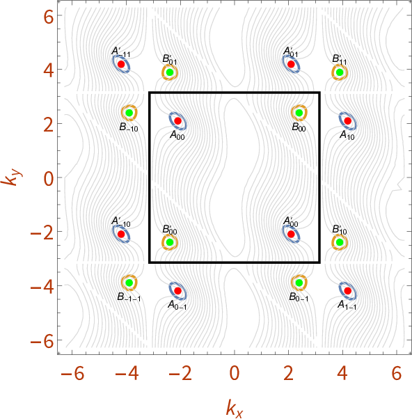
For $0<t^{\prime}<1$ , there are exactly four Dirac contact points per Brillouin zone, which can be grouped into couples: we write $B$ , $B^{\prime}$ , Dirac points that are located in the diagonal $k_{x}=k_{y}\ ({\rm mod}\;2\pi)$ and correspond to contact points between the two upper bands $e_{1}$ and $e_{0}$ ; we write $A$ , $A^{\prime}$ , those located in the antidiagonal $k_{x}={-}k_{y}\ ({\rm mod}\;2\pi)$ and which correspond to contact points between the two lower bands $e_{\sm 1}$ and $e_{1}$ .

Taking into account $(2\pi,0)$ and $(0,2\pi)$ translations, contact points range in the whole reciprocal space. Those of $A$ , $A^{\prime}$ kind write $A_{mn}{=}(\alpha_{t^{\prime}}+2\,\!m\,\!\pi,{-}\alpha_{t^{\prime}}+2\,\!n\,\!\pi)\!\!$ and $A^{\prime}_{mn}{=}({-}\alpha_{t^{\prime}}+2\,\!m\,\!\pi,\alpha_{t^{\prime}}+2\,\!n\,\!\pi)$ , with $\alpha_{t^{\prime}}=2\cos^{-1}(t^{\prime})$ for any integers $(m,n)\in\mathbb{Z}^{2}$ . Those of $B$ , $B^{\prime}$ kind write $B_{mn}{=}(\beta_{t^{\prime}}{+}2\,\!m\,\!\pi,\beta_{t^{\prime}}{+}2\,\!n\,\!\pi)$ and $B^{\prime}_{mn}{=}({-}\beta_{t^{\prime}}{+}2\,\!m\,\!\pi,$ ${-}\beta_{t^{\prime}}{+}2\,\!n\,\!\pi)$ , with $\beta_{t^{\prime}}=2\cos^{-1}\!\Big(\frac{\sqrt{1+8t^{\prime 2}}-1}{4t^{\prime}}\Big)$ for any integers $(m,n)\in\mathbb{Z}^{2}$ . We show some of these points for $t^{\prime}=\frac{1}{2}$ in the following representation Fig. 4 of energy differences in an extended reciprocal space zone:

Contact points move while $t^{\prime}$ describes interval $[0,1]$ . For $t^{\prime}=0$ , one finds $\alpha_{0}=\beta_{0}=\pi$ , so points $A_{00}$ , $A^{\prime}_{\sm 11}$ , $B_{\sm 10}$ and $B^{\prime}_{01}$ merge altogether into a unique singularity at point $M_{00}$ , where we define $M_{mn}=((2m+1)\pi,$ $(2n+1)\pi)$ . Similar mergings occur modulo $2\pi$ in each $k_{x}$ and $k_{y}$ directions. For $t^{\prime}=1$ , $\beta_{1}=\frac{2\pi}{3}$ and $\alpha_{1}=0$ , so points $A_{00}$ and $A^{\prime}_{00}$ merge into a unique singularity at point $\Gamma_{00}$ , where we define $\Gamma_{mn}=(2m\pi,2n\pi)$ . Similar mergings occur modulo $2\pi$ in each $k_{x}$ and $k_{y}$ directions. One can also mention interesting value $\alpha_{\frac{1}{2}}=\frac{2\pi}{3}$ . This is resumed in Fig. 5:

Eigenstates

We write $|v_{n}\rangle$ each eigenvector corresponding to energy $e_{n}$ , $\forall n={-}1,0,1$ . The column vector writes

\!\!\!\!\!\!\!\!\!\!v_{n}(k_{x},k_{y})=\pmatrix{\cos\!\big(\!\frac{k_{x}}{2}\!\big)\cos\!\big(\!\frac{k_{y}}{2}\!\big)+\frac{t^{\prime}}{2}\cos\!\big(\!\frac{k_{x}+k_{y}}{2}\!\big)e_{n}(k_{x},k_{y})\cr{-}\cos\!\big(\!\frac{k_{x}}{2}\!\big)^{2}+\frac{1}{4}e_{n}(k_{x},k_{y})^{2}\cr t^{\prime}\cos\!\big(\!\frac{k_{x}}{2}\!\big)\cos\!\big(\!\frac{k_{x}+k_{y}}{2}\!\big)+\frac{1}{2}\cos\!\big(\!\frac{k_{y}}{2}\!\big)e_{n}(k_{x},k_{y})\cr}.

These expressions are not normalized, so one needs to use $|v_{n}\rangle/\sqrt{\langle v_{n}|v_{n}\rangle}$ in order to get normalized vectors. To each $|v_{n}\rangle$ corresponds a projector $\Pi_{n}=\frac{|v_{n}\rangle\langle v_{n}|}{\langle v_{n}|v_{n}\rangle}$ . We decompose $\Pi_{n}$ into Bloch components $a^{1}_{n}$ , …, $a^{8}_{n}$ such that:

\Pi_{n}=\frac{1}{3}{\cal I}+\frac{1}{\sqrt{3}}\sum_{i=1}^{8}a^{i}_{n}\lambda_{i}

with the Gell-Mann matrices:
$\lambda_{1}=\pmatrix{0&1&0\cr 1&0&0\cr 0&0&0\cr}$ ; $\lambda_{2}=\pmatrix{0&{-}\mathbbm{i}&0\cr\mathbbm{i}&0&0\cr 0&0&0\cr}$ ; $\lambda_{3}=\pmatrix{1&0&0\cr 0&{-}1&0\cr 0&0&0\cr}$ ; $\lambda_{4}=\pmatrix{0&0&1\cr 0&0&0\cr 1&0&0\cr}$ ; $\lambda_{5}=\pmatrix{0&0&{-}\mathbbm{i}\cr 0&0&0\cr\mathbbm{i}&0&0\cr}$ ; $\lambda_{6}=\pmatrix{0&0&0\cr 0&0&1\cr 0&1&0\cr}$ ; $\lambda_{7}=\pmatrix{0&0&0\cr 0&0&{-}\mathbbm{i}\cr 0&\mathbbm{i}&0\cr}$ ; $\lambda_{8}=\displaystyle\frac{1}{\sqrt{3}}\pmatrix{1&0&0\cr 0&1&0\cr 0&0&{-}2\cr}$ .

3 Determination of the universal classification surface

Calculations with projectors provide phase independent results, contrary to vector based ones. We will, in particular, ensure that they account for the correct number of degrees of freedom, altogether.

3.1 One projector conditions

Let us introduce equation

a.a=1\quad\hbox{and}\quad a\star a=a\;,

(1)

where $a=(a^{1},...,a^{8})$ is the Bloch octuplet describing an eigenstate, $a.b=\sum_{i=1}^{8}a^{i}b^{i}$ is a scalar product and the star product $a\star b$ is defined by $a\star b=\sum_{i=1}^{8}a^{j}b^{k}d_{ijk}$ with

	$\displaystyle d_{ii8}=d_{i8i}=d_{8ii}=\frac{1}{\sqrt{3}}\qquad\forall i=1,2,3\;;$
	$\displaystyle d_{ii8}=d_{i8i}=d_{8ii}={-}\frac{1}{2\sqrt{3}}\quad\forall i=4,..,7\;;$
	$\displaystyle d_{888}={-}\frac{1}{\sqrt{3}}\;;$
	$\displaystyle d_{146}=d_{461}=d_{614}=d_{164}=d_{641}=d_{416}=\frac{1}{2}\;;$
	$\displaystyle d_{157}=d_{571}=d_{715}=d_{175}=d_{751}=d_{517}=\frac{1}{2}\;;$
	$\displaystyle d_{256}=d_{562}=d_{625}=d_{265}=d_{652}=d_{526}=\frac{1}{2}\;;$
	$\displaystyle d_{344}=d_{434}=d_{443}=d_{355}=d_{535}=d_{553}=\frac{1}{2}\;;$
	$\displaystyle d_{247}=d_{472}=d_{724}=d_{274}=d_{742}=d_{427}={-}\frac{1}{2}\;;$
	$\displaystyle d_{366}=d_{636}=d_{663}=d_{377}=d_{737}=d_{773}={-}\frac{1}{2}\;.$

Each projector $\Pi_{n}$ respects²⁹ (1), with $a=a_{n}$ , $\forall n={-}1,0,1$ .

Let us study (1) formally. After some tedious calculations, one finds that it is equivalent to the five equations

$\displaystyle(a^{4})^{2}+(a^{5})^{2}+(a^{6})^{2}+(a^{7})^{2}$
$\displaystyle+\frac{4}{3}\Big(a^{8}+\frac{1}{4}\Big)^{2}$	$\displaystyle=$	$\displaystyle\frac{3}{4}\;;$	(2)
$\displaystyle(a^{1})^{2}+(a^{2})^{2}+(a^{3})^{2}$	$\displaystyle=$	$\displaystyle\frac{1}{3}(a^{8}+1)^{2}\;;$	(3)
$\displaystyle\sqrt{3}(a^{4}a^{6}+a^{5}a^{7})$	$\displaystyle=$	$\displaystyle(1-2a^{8})a^{1}\;;$	(4)
$\displaystyle\sqrt{3}(a^{5}a^{6}-a^{4}a^{7})$	$\displaystyle=$	$\displaystyle(1-2a^{8})a^{2}\;;$	(5)
$\displaystyle\sqrt{3}\big((a^{4})^{2}+(a^{5})^{2}-(a^{6})^{2}-(a^{7})^{2}\big)$	$\displaystyle=$	$\displaystyle 2(1-2a^{8})a^{3}.$	(6)

All coordinates in $v_{n}(k_{x},k_{y})$ are actually real, so there is no imaginary term in their Bloch decomposition. Therefore, $a^{2}=0$ , $a^{5}=0$ and $a^{7}=0$ for all $a=a_{n}$ , with $n=-1,0,1$ , and we discard these three components in the whole article hereafter. Equations (2), (4) and (6) become

$\displaystyle(a^{4})^{2}+(a^{6})^{2}+\frac{4}{3}\Big(a^{8}+\frac{1}{4}\Big)^{2}$	$\displaystyle=$	$\displaystyle\frac{3}{4}\;;$	(7)
$\displaystyle\sqrt{3}a^{4}a^{6}$	$\displaystyle=$	$\displaystyle(1-2a^{8})a^{1}\;;$	(8)
$\displaystyle\sqrt{3}\big((a^{4})^{2}-(a^{6})^{2}\big)$	$\displaystyle=$	$\displaystyle 2(1-2a^{8})a^{3}\;.$	(9)

We have skipped (3), which becomes redundant and (5), which becomes trivial. Altogether, for each projector $\Pi_{n}$ , there are five degrees of freedom, constrained to the three equations (7), (8) and (9) applied with $a=a_{n}$ . Therefore, we are left with two degrees for each projector. In the following, we will keep $a^{4}_{n}$ and $a^{6}_{n}$ for each $n={-1},0,1$ , using (7) to express $a^{8}_{n}$ in terms of $a^{4}_{n}$ and $a^{6}_{n}$ , then (8) to express $a^{1}_{n}$ in terms of $a^{4}_{n}$ and $a^{6}_{n}$ and similarly (9) to express $a^{3}_{n}$ in terms of $a^{4}_{n}$ and $a^{6}_{n}$ . We are left with $6=3\times 2$ components, $\{a^{4}_{\sm 1},a^{6}_{\sm 1},a^{4}_{0},a^{6}_{0},a^{4}_{1},a^{6}_{1}\}$ , which exceeds three, the maximal number of free parameters. One must now take orthogonality relations into account in order to discard irrelevant ones.

3.2 Two projector conditions

For each projector $\Pi_{n}$ , with $n={-}1,0,1$ , the standard relations $\Pi_{n}\Pi_{n}=\Pi_{n}$ are already embedded in relations (7), (8) and (9). We will now examine mutual relations between projectors.

3.2.1 Completeness relation

First of all, they follow

\Pi_{\sm 1}+\Pi_{1}+\Pi_{0}={\,\rm Id},

(10)

so one of them is determined by the others; (10) writes

a^{4}_{p}=-a^{4}_{m}-a^{4}_{n}\quad\hbox{and}\quad a^{6}_{p}=-a^{6}_{m}-a^{6}_{n}\;,

(11)

where $\{m,n,p\}$ is a permutation of $\{{-}1,0,1\}$ ; in other words $m=\sigma({-}1)$ , $n=\sigma(0)$ and $p=\sigma(1)$ with $\sigma\in{\rm Sym}(\{-1,0,1\})$ an arbitrary permutation. (11) discards two free parameters, so the actual counting of degrees of freedom already drops to four.

3.2.2 Other relations reduce to a unique equation

All other relations will reduce to a unique equation, which we introduce at once: consider any arbitrary octuplets $a$ and $b$ , it writes

a.b={-}\frac{1}{2}\quad\hbox{and}\quad a\star b={-}a-b\;.

(12)

We will prove now that condition: “ $\forall i\neq j$ , $\Pi_{i}.\Pi_{j}=0$ ” is equivalent to (12), with $a=a_{m}$ and $b=a_{n}$ , where $\{m,n,p\}$ are defined above and keeping in mind that all components $a^{i}_{p}$ can express in terms of $(a^{4}_{m},a^{6}_{m},a^{4}_{n},a^{6}_{n})$ , thanks to (11).

Let us first study (12) formally. This again gives tedious calculations; several particular cases arise, which separate from the general solution. Let us give two of them. The first one leads to equations

\left\{\begin{tabular}[]{l}$a^{8}=b^{8}=\frac{1}{2}$,\quad$a^{4}=a^{6}=b^{4}=b^{6}=0$,\\ $b^{1}={-}a^{1}$,\quad$b^{3}={-}a^{3}$\\ and $(a^{1})^{2}+(a^{3})^{2}=\frac{3}{4}$.\end{tabular}\right.

(13)

The second one leads to equations

\left\{\begin{tabular}[]{l}$a^{8}=b^{8}={-}\frac{1}{4}$,\quad$b^{4}={-}a^{4}$,\quad$b^{6}={-}a^{6}$,\\ $b^{1}=a^{1}=\displaystyle\frac{2a^{4}a^{6}}{\sqrt{3}}$,\quad$b^{3}=a^{3}=\displaystyle\frac{(a^{4})^{2}-(a^{6})^{2}}{\sqrt{3}}$\\ and\quad$(a^{4})^{2}+(a^{6})^{2}=\frac{3}{4}$.\end{tabular}\right.

(14)

Other cases exist, which study is irrelevant here. Keeping Lieb case $t^{\prime}=0$ apart, which needs special investigations, all particular situations only arise for $k_{x}=k_{y}\ ({\rm mod}\;\;\pi)$ or for $k_{x}={-}k_{y}\ ({\rm mod}\;\;\pi)$ , at all $t^{\prime}>0$ . These lines merge into the plan, letting all components behave analytically, so we can ignore them. Let us eventually give the generic solution of (12); we first introduce coordinates $X$ , $Y$ and $Z=V+W$ :

$\displaystyle X(a^{4},a^{6},b^{4},b^{6})$	$\displaystyle=$	$\displaystyle a^{4}b^{4}+a^{6}b^{6}\;,$
$\displaystyle Y(a^{4},a^{6},b^{4},b^{6})$	$\displaystyle=$	$\displaystyle a^{6}b^{4}-a^{4}b^{6}\;,$
$\displaystyle V(a^{4},a^{6},b^{4},b^{6})$	$\displaystyle=$	$\displaystyle(a^{4})^{2}+(b^{4})^{2}$
$\displaystyle\hbox{and}\quad W(a^{4},a^{6},b^{4},b^{6})$	$\displaystyle=$	$\displaystyle(a^{6})^{2}+(b^{6})^{2}\;.$

Then, the generic solution of (12) writes

3X^{2}Z+6X^{3}+3XY^{2}+Y^{4}=0\;,

(15)

while all other components are given by

	$\displaystyle a^{1}={-}\frac{a^{4}a^{6}Y^{2}}{\sqrt{3}X(X+V)}\;,$		$\displaystyle b^{1}={-}\frac{b^{4}b^{6}Y^{2}}{\sqrt{3}X(X+W)}\;,$
	$\displaystyle a^{3}=\frac{((a^{6})^{2}-(a^{4})^{2})Y^{2}}{2\sqrt{3}X(X+V)}\;,$		$\displaystyle b^{3}=\frac{((b^{6})^{2}-(b^{4})^{2})Y^{2}}{2\sqrt{3}X(X+W)}\;,$
	$\displaystyle a^{8}=\frac{(3X+W)V+2X^{2}}{2Y^{2}}\;,$		$\displaystyle b^{8}=\frac{(3X+V)W+2X^{2}}{2Y^{2}}\;,$

where the dependency in $(a^{4},a^{6},b^{4},b^{6})$ is hidden. Taking into account (15) with $a=a_{m}$ and $b=a_{n}$ , we have proven that the number of degrees of freedom is exactly three.

4 Classification of singularities

Following previous work,^{21, 22, 30, 23} we characterize topological singularities of the energy band structure by mapping closed paths from reciprocal space onto surface $\cal S$ . This mapping writes $\gamma\to{\mathop{\widetilde{\gamma}}}$ , where $\gamma$ is defined in reciprocal space and ${\mathop{\widetilde{\gamma}}}$ in $\cal S$ , and defines a subgroup of the fundamental group $\pi_{1}({\cal S})$ .

4.1 Description of universal classification surface $\cal S$

Let $(m,n,p)$ be some permutation of $\{-1,0,1\}$ as already defined, we recall that (11) allows one to skip all $a^{i}_{p}$ components, so all Bloch components express in terms of $(a^{4}_{m},a^{6}_{m},a^{4}_{n},a^{6}_{n})$ , while (12), applied with $a=a_{m}$ and $b=a_{n}$ , dismissing non generic cases, proves that these components are not free and live in surface $\cal S$ , defined by (15), which writes explicitly

	$\displaystyle 3(a^{4}_{m}a^{4}_{n}+a^{6}_{m}a^{6}_{n})^{2}\big((a^{4}_{m})^{2}{+}(a^{4}_{n})^{2}{+}(a^{6}_{m})^{2}{+}(a^{6}_{n})^{2}\big)$
	$\displaystyle+6(a^{4}_{m}a^{4}_{n}+a^{6}_{m}a^{6}_{n})^{3}+3(a^{4}_{m}a^{4}_{n}+a^{6}_{m}a^{6}_{n})\times$
	$\displaystyle(a^{6}_{m}a^{4}_{n}-a^{4}_{m}a^{6}_{n})^{2}+(a^{6}_{m}a^{4}_{n}-a^{4}_{m}a^{6}_{n})^{4}=0\;.$

$\cal S$ is a tridimensional surface embedded in the 4-dimension space spanned by components $(a^{4}_{m},a^{6}_{m},a^{4}_{n},a^{6}_{n})$ . It does not depend on $t^{\prime}$ . A direct description seems, at first, not available but we have been lucky enough to find out that there is a singularity at point $O=(0,0,0,0)$ . Its determination is explained in appendix, however, its properties have been redundantly proven afterwards, as will now be explained.

Several 4-dimensional connected volumes, cone-shaped, lying outside of $\cal S$ , point towards the origin $O$ . They form holes joining at $O$ . To explore this net of holes, we draw the intersection of $\cal S$ with $r$ - $S_{3}$ , the 3-sphere of radius $r$ , using Hopf coordinates:

$\displaystyle a^{4}_{m}$	$\displaystyle=$	$\displaystyle r\cos t\cos u\;,$
$\displaystyle a^{4}_{n}$	$\displaystyle=$	$\displaystyle r\cos t\sin u\;,$
$\displaystyle a^{6}_{m}$	$\displaystyle=$	$\displaystyle r\sin t\cos v\;,$
$\displaystyle a^{6}_{n}$	$\displaystyle=$	$\displaystyle r\sin t\sin v\;,$

with $0\leq t<\pi/2$ , ${-}\pi<u\leq\pi$ and ${-}\pi<v\leq\pi$ . This intersection does not vary with $r$ , when $r$ ranges interval $]0,\sqrt{\phantom{\!\bar{\hat{\gamma}}}}\hskip-5.0pt\frac{3}{2}]$ . One observes 18 toroidal holes, as seen in Fig. 6. Detailed folding rules are given in appendix, as well as the counting of all holes. 12 holes are parallel to $t$ -axis, 3 parallel to $u$ -axis and 3 to $v$ -axis.

We do not need to determine the exact topology of $\cal S$ and to investigate how holes relate one to the other. As shown in Fig. 7, whatever the values of $(m,n)$ , mapping $(k_{x},k_{y})\mapsto(a^{4}_{m},a^{6}_{m},a^{4}_{n},a^{6}_{n})$ spreads over a volume smaller than $\cal S$ , which we call effective classification surface. In Fig. 8, one observes that the 12 holes inside $\cal S$ , parallel to $t$ -axis, are enough to characterize the topology of all paths generated by mapping $\gamma\to{\mathop{\widetilde{\gamma}}}$ . Indeed, any path turning around one of these twelve holes cannot retract towards a trivial one, and the first homotopy group is defined by the number of windings around holes. We will henceforth use a schematic view of Fig. 6 (a), presented in Fig. 9, where the twelve corresponding holes are represented as large or small circles.

Detailed results are given in section “Classification and winding numbers” but we discuss at once the choice of permutation $\{m,n,p\}$ . Let us deal with choices $(m,n)=(0,1)$ , $(m,n)=({-}1,1)$ and $(m,n)=({-}1,0)$ (we skip index $p$ which can be deduced), the three others giving identical results. With $(m,n)=({-}1,0)$ , indices of upper and lower bands, the effective classification surface is represented on Figs. 7 (a) and 8 (a); all paths ${\mathop{\widetilde{\gamma}}}$ turn around a hole corresponding to a small circle in Fig. 9, which are labelled from $C$ to $J$ . If one of indices $(m,n)$ is 1 –the index of the middle band–, effective classification surfaces for both choices are represented on Figs. 7 (b) and 8 (b); all paths ${\mathop{\widetilde{\gamma}}}$ turn around a hole correspond to a large circle or a small circle (among $\{D,F,H,J\}$ ) in Fig. 9.

From now on, we definitely choose $m={-1}$ , $n=0$ (thus $p=1$ ). The validity of the topological classification will be established thanks to the mapping into $\cal S$ , yet one may use easier representations. Therefore, we will now give two alternatives to mapping $\gamma\to{\mathop{\widetilde{\gamma}}}$ , defined in surfaces of smaller dimensions.

4.2 Bidimensional surface $\widetilde{\cal S}_{1}$

This representation is efficient only with $(m,n)=({-}1,0)$ (or $(m,n)=(0,{-}1)$ ), not with $m=1$ or $n=1$ . Since all expressions are symmetric or antisymmetric with the exchange $a_{m}\leftrightarrow a_{n}$ , we keep $m={-}1$ and $n=0$ as for $\cal S$ .

4.2.1 $\widetilde{\cal S}_{1}$ is a projection of $\cal S$

We construct surface $\widetilde{\cal S}_{1}$ as a projection of $\cal S$ , through the two separate mappings $\tau_{a}$ and $\tau_{d}$ :

	$\displaystyle\tau_{a}:\quad$	$\displaystyle(a^{4}_{\sm 1},a^{6}_{\sm 1},a^{4}_{0},a^{6}_{0})$	$\displaystyle\mapsto(a^{4}_{\sm 1},a^{6}_{\sm 1})\;,$
	$\displaystyle\tau_{d}:\quad$	$\displaystyle(a^{4}_{\sm 1},a^{6}_{\sm 1},a^{4}_{0},a^{6}_{0})$	$\displaystyle\mapsto(a^{4}_{0},a^{6}_{0})\;,$

where $a$ stands for antidiagonal and $d$ for diagonal, giving two disconnected bidimensional surfaces. Both have an equal inverted four-leaf clover shape with four holes (one hole inside each leaf); we call $\cal Q$ the generic surface, having such shape, which can be described by equation

	$\displaystyle\forall(a^{4})^{2}+(a^{6})^{2}$	$\displaystyle\leq$	$\displaystyle\frac{3}{4}$		(16)
	$\displaystyle\scriptstyle 6\big(\!(a^{4})^{2}+(a^{6})^{2}\!\big)^{4}+\big(\!(a^{4})^{2}-(a^{6})^{2}\!\big)^{4}$	$\displaystyle\leq$	$\displaystyle\scriptstyle\frac{205}{43}\big(\!(a^{4})^{2}-(a^{6})^{2}\!\big)^{2}-\frac{1}{3}\big(\!(a^{4})^{2}+(a^{6})^{2}\!\big)^{2}$

so that $\widetilde{\cal S}_{1}={\cal Q}_{a}\times{\cal Q}_{d}$ , where ${\cal Q}_{a}=\tau_{a}({\cal S})$ and ${\cal Q}_{d}=\tau_{d}({\cal S})$ . Eventually, we will find that $\tau_{a}({\mathop{\widetilde{\gamma}}})$ are non trivial only when $\gamma$ circles a contact point between lower and middle bands; while $\tau_{d}({\mathop{\widetilde{\gamma}}})$ are non trivial only when $\gamma$ circles a contact point between upper and middle bands, as shown in Fig. 10. $\tau_{a}\times\tau_{d}$ is surjective, yet we will see that it preserves the whole topological classification. We introduce the complex notation: $z_{1a}=a^{6}_{\sm 1}+\mathbbm{i}\,a^{4}_{\sm 1}$ and $z_{1d}=a^{6}_{0}+\mathbbm{i}\,a^{4}_{0}$ for further investigations.

4.2.2 Validity

Bloch components $(a^{4}_{m},a^{6}_{m})$ follow (16) for all $t\in[0,1]$ and $m={-}1$ or $m=0$ , but not for $m=1$ . Coefficients in (16) are deduced from a numerical determination of $\widetilde{\cal S}_{1}$ and must be improved. Although their exact determination is still lacking, confidence in the inverted four-leaf clover shape and in the properties of ${\cal Q}$ is complete, because our numerical determination is actually exact. ${\cal Q}$ is embedded in a bidimensional space and reveals a singular point, as shown in Fig. 10. Moreover, the outer circular edge is exactly determined and corresponds to limit $t^{\prime}=0$ , as we shall see.

4.2.3 Symbolic notations of non trivial loops in $\widetilde{\cal S}_{1}$

Except for some trivial way and return loops, that exhibit two flip points, all paths $\tau_{i}({\mathop{\widetilde{\gamma}}})$ in $\widetilde{\cal S}_{1}$ , with any $i=a,d$ , are continuous; in particular, consider a non trivial path $\tau_{i}({\mathop{\widetilde{\gamma}}})$ which goes across the singularity, $(0,0)\in\tau_{i}({\mathop{\widetilde{\gamma}}})$ , then $\tau_{i}({\mathop{\widetilde{\gamma}}})$ follows necessarily two consecutive leaves of the clover, therefore it can not retract. In order to distinguish these path, we will write $\dlsh$ , $\drsh$ , $\Lsh$ , $\Rsh$ , $\Lsh$ , $\dlsh$ , $\Rsh$ , $\drsh$ , where each segment stands for the leaf enveloping it, their intersection for $(0,0)$ , and the arrow for the direction of path $\tau_{i}({\mathop{\widetilde{\gamma}}})$ . For instance, the path in Fig. 10 writes $\tau_{d}({\mathop{\widetilde{\gamma}}})=$ $\drsh$ . Note that there are other non trivial loops, which we will study further on.

4.2.4 Definition of winding number $\omega_{1}$

We define $\omega_{1}$ in $\widetilde{\cal S}_{1}$ as follow. We use a special convention, which allows a nice continuation with the winding number defined in Lieb model. Consider a loop $\gamma$ in reciprocal space which maps into loops $\tau_{a}({\mathop{\widetilde{\gamma}}})=(a^{4}_{\sm 1}(k_{x},k_{y}),$ $a^{6}_{\sm 1}(k_{x},k_{y}))$ and $\tau_{d}({\mathop{\widetilde{\gamma}}})=(a^{4}_{0}(k_{x},k_{y}),$ $a^{6}_{0}(k_{x},k_{y}))$ .

We will here only consider non trivial two-leaf paths as $\dlsh$ , $\drsh$ , $\Lsh$ , $\Rsh$ , $\Lsh$ , $\dlsh$ , $\Rsh$ or $\drsh$ . Assuming that ${\cal Q}_{a}$ and ${\cal Q}_{d}$ are orientated with their normal pointing in front of Fig. 10, $\tau_{a}({\mathop{\widetilde{\gamma}}})$ and $\tau_{d}({\mathop{\widetilde{\gamma}}})$ are counted positively if they turn in the trigonometric direction and negatively if they turn in the reverse direction. Then we set $\omega_{1}$ as the sum of all windings associated to each path $\tau_{a}({\mathop{\widetilde{\gamma}}})$ or $\tau_{d}({\mathop{\widetilde{\gamma}}})$ and defined as follow : $\frac{1}{4}$ for $\drsh$ , $\Lsh$ , $\Lsh$ or $\drsh$ ; and ${-}\frac{1}{4}$ for $\dlsh$ , $\Rsh$ , $\Rsh$ or $\dlsh$ . All such paths turn around singularities $(0,0)$ in ${\cal Q}_{a}$ or ${\cal Q}_{d}$ , but their non triviality is proven by the non triviality of ${\mathop{\widetilde{\gamma}}}$ in $\cal S$ . This convention is arbitrary but leads to very convenient connecting rules, in particular for limits $t^{\prime}\to 0$ and $t^{\prime}\to 1$ and matches further convention of winding number $\omega_{4}$ . Other non trivial loops can be observed, that will be examined further on, but they can be decomposed into these ones, so our definition of $\omega_{1}$ is complete.

As will be explained further on, the homotopy classification on $\widetilde{\cal S}_{1}$ is equivalent to that on $\cal S$ , although $\omega_{1}$ gives only very partial information. On the contrary, the next four surfaces ${\cal S}_{2}$ , ${\cal R}^{\prime}$ , $\cal C$ and $\cal T$ only provide partial classification separately. We will define four corresponding winding numbers $(\omega_{2},\omega_{3},\omega_{4},\omega_{5})$ associated to each one. Eventually, we will show that topological properties are correctly described when the set ${\cal E}={\cal S}_{2}\times{\cal R}\times{\cal C}\times\cal T$ (see differences between $\cal R$ and ${\cal R}^{\prime}$ afterwards) is used as a space of classification, with quadruple index $(\omega_{2},\omega_{3},\omega_{4},\omega_{5})$ .

4.3 Surface ${\cal S}_{2}$

Let us consider ${\cal S}_{2}$ , the first compound in $\cal E$ : it is a bidimensional surface described by equation (15) as a function of $(X,Y,Z)$ , recalling $Z=V+W$ . ${\cal S}_{2}$ is embedded in a tridimensional space and reveals a singular point, as shown in Fig. 11.

4.3.1 ${\cal S}_{2}$ is a projection of $\cal S$

We construct projection $s$ , ${\cal S}\to{\cal S}_{2}$ , $s(a^{4}_{m},a^{6}_{m},a^{4}_{n},a^{6}_{n})$ $=\big(X(a^{4}_{m},a^{6}_{m},a^{4}_{n},a^{6}_{n}),Y(a^{4}_{m},a^{6}_{m},a^{4}_{n},a^{6}_{n}),Z(a^{4}_{m},a^{6}_{m},a^{4}_{n},a^{6}_{n})\big)$ , so ${\cal S}_{2}=s({\cal S})$ . A loop $\gamma$ in reciprocal space maps into $\gamma_{2}=s({\mathop{\widetilde{\gamma}}})$ in ${\cal S}_{2}$ . Consider a path $\gamma$ , turning around a contact point, then $\gamma_{2}$ turns around $O=(0,0,0)$ , the singularity of ${\cal S}_{2}$ ; the non triviality of $\gamma_{2}$ is proven by that of ${\mathop{\widetilde{\gamma}}}$ . Indeed, it is not possible to reduce $\gamma_{2}$ continuously without crossing $O$ . On the contrary, $\gamma_{2}$ (and ${\mathop{\widetilde{\gamma}}}$ , see however 4.8.6) can retract when the surface delimited by $\gamma$ does not contain any contact point, see Fig. 11. We choose $m={-}1$ and $n=0$ , as already discussed: other choices prove either equivalent or inefficient.

4.3.2 Definition of winding number $\omega_{2}$

This mapping defines winding number $\omega_{2}$ , which counts algebraically the number of loops of $\gamma_{2}$ . Surface ${\cal S}_{2}$ is opened, thus its normal can be chosen arbitrarily; therefore, $\omega_{2}$ is defined up to a global sign. Assuming that ${\cal S}_{2}$ is orientated with its normal pointing in front of Fig. 11, $s({\mathop{\widetilde{\gamma}}})$ is counted positively if it turns in the trigonometric direction and negatively if it turns in the reverse direction.

4.3.3 Range of parameters $X$ , $Y$ and $Z$

One observes that parameters $X$ and $Y$ spread over smaller range than what could be expected from their definition. Indeed, $X(a^{4}_{m}(k_{x},k_{y}),a^{6}_{m}(k_{x},k_{y}),a^{4}_{n}(k_{x},k_{y}),$ $a^{6}_{n}(k_{x},k_{y}))\in[{-}\frac{3}{4},0]$ and $Y(a^{4}_{m}(k_{x},k_{y}),a^{6}_{m}(k_{x},k_{y}),$ $a^{4}_{n}(k_{x},k_{y}),a^{6}_{n}(k_{x},k_{y}))\in[{-}\frac{1}{\sqrt{3}},\frac{1}{\sqrt{3}}]$ for all $(k_{x},k_{y})$ , with $m={-}1$ and $n=0$ . This is not true when $m=1$ or $n=1$ . In particular, one has $\forall(k_{x},k_{y})\in\mathbb{R}^{2}$ ,

X(a^{4}_{\sm 1}(k_{x},k_{y}),a^{6}_{\sm 1}(k_{x},k_{y}),a^{4}_{0}(k_{x},k_{y}),a^{6}_{0}(k_{x},k_{y}))\leq 0\;.

(17)

On the contrary, the range of parameter $Z$ is conform to what can be deduced from its definition, $\forall(m,n)\in\{{-}1,0,1\}$ :

Z(a^{4}_{m}(k_{x},k_{y}),a^{6}_{m}(k_{x},k_{y}),a^{4}_{n}(k_{x},k_{y}),a^{6}_{n}(k_{x},k_{y}))\in[0,\frac{3}{2}]

4.4 Surface $\cal R$

We now examine $\cal R$ , the second compound in $\cal E$ . It is defined through ${\cal R}^{\prime}$ , which is embedded in a bidimensional space and reveals two singular points, as shown in Fig. 12.

4.4.1 ${\cal R}^{\prime}$ is a projection of $\cal S$

We construct projection $r$ from $\cal S$ to ${\cal R}^{\prime}$ , $r(a^{4}_{\sm 1},a^{6}_{\sm 1},a^{4}_{0},a^{6}_{0})=(a^{4}_{\sm 1}+a^{4}_{0},a^{8}_{\sm 1}+a^{8}_{0})$ , so ${\cal R}^{\prime}=r({\cal S})$ . This surface is embedded in an ellipse with semi-major axis along $Ox$ of length $\frac{\sqrt{3}}{2}$ and semi-minor axis along $Oy$ of length $\frac{3}{4}$ , and center $(0,\frac{1}{4})$ , see Fig. 12. Two parts are removed, forming ellipses, inclined by $\pm\frac{\pi}{5}$ , of equations

\scriptstyle\frac{9}{4}\big((x-\frac{1}{2\sqrt{3}})\cos\frac{\pi}{5}+y\sin\frac{\pi}{5}\big)^{2}+\frac{64}{9}\big((x-\frac{1}{2\sqrt{3}})\sin\frac{\pi}{5}-y\cos\frac{\pi}{5}\big)^{2}\leq 1\;,

\scriptstyle\frac{9}{4}\big((x+\frac{1}{2\sqrt{3}})\cos\frac{\pi}{5}-y\sin\frac{\pi}{5}\big)^{2}+\frac{64}{9}\big((x+\frac{1}{2\sqrt{3}})\sin\frac{\pi}{5}+y\cos\frac{\pi}{5}\big)^{2}\leq 1\;,

(18)

except their intersection, which lies inside ${\cal R}^{\prime}$ . Altogether, there are two holes indeed in ${\cal R}^{\prime}$ .

4.4.2 Validity

Confidence in the general shape and in the properties of ${\cal R}^{\prime}$ is complete, because our numerical determination is actually exact. However, some hints indicate that the coefficients in (18) must be improved, see the discussion about surface $\widetilde{\cal T}$ in appendix. The elliptic outer edge is exactly determined by equations (7), (8) and (9) and corresponds to limit $t^{\prime}=0$ .

4.4.3 Definition of winding number $\omega_{3}$

Assuming that ${\cal R}^{\prime}$ is orientated with its normal pointing in front of Fig. 12, $r({\mathop{\widetilde{\gamma}}})$ is counted positively if it turns in the trigonometric direction and negatively if it turns in the reverse direction. Then we set $\omega_{3}$ as the sum of all windings around any of the two holes. For instance, a path turning once in the trigonometric direction and enclosing both holes gives $\omega_{3}=2$ .

$\omega_{3}$ does not separate a path turning around one hole from that turning around the other. Let us define a second winding $\widetilde{\omega}_{3}$ , that still does not separate holes, but a path around the right hole (such that horizontal coordinate $x>0$ in Fig. 12) is counted positively, while a path around the left hole is counted negatively. For instance, a path enclosing both holes gives $\widetilde{\omega}_{3}=0$ .

One can verify that $(\omega_{3},\widetilde{\omega}_{3})$ captures the whole topology of ${\cal R}^{\prime}$ . In appendix, we define quotient spaces $\cal R$ and $\widetilde{\cal R}$ , which are associated to, respectively, winding numbers $\omega_{3}$ and $\widetilde{\omega}_{3}$ . ${\cal R}^{\prime}$ is homotopically equivalent to ${\cal R}\times\widetilde{\cal R}$ , one finds $\widetilde{\omega}_{3}=-\omega_{5}$ and the hole, around which $r({\mathop{\widetilde{\gamma}}})$ turns, is given by $-\omega_{3}\omega_{5}$ with the convention that it is the right hole if $-\omega_{3}\omega_{5}>0$ and the left hole if $-\omega_{3}\omega_{5}<0$ .

4.5 Surface $\cal C$

We now examine $\cal C$ , the third compound in $\cal E$ . $\cal C$ is embedded in a bidimensional space and reveals two singular points, as shown in Fig. 13.

4.5.1 $\cal C$ is a projection of $\cal S$

We construct projection $c$ from $\cal S$ to $\cal C$ , $c(a^{4}_{\sm 1},a^{6}_{\sm 1},a^{4}_{0},a^{6}_{0})=(a^{3}_{\sm 1}a^{1}_{0}+a^{1}_{\sm 1}a^{3}_{0},a^{3}_{\sm 1}a^{3}_{0}-a^{1}_{\sm 1}a^{1}_{0})$ , so ${\cal C}=c({\cal S})$ . Using complex notation $z_{1}$ and ignoring scaling factors $\frac{-Y^{2}}{2\sqrt{3}(X+V)}$ or $\frac{-Y^{2}}{2\sqrt{3}(X+W)}$ , it writes $(z_{1a},z_{1d})\mapsto\overline{(z_{1a}z_{1d})}^{2}$ . One could alternatively study the surface defined by the mapping
$(a^{4}_{\sm 1},a^{6}_{\sm 1},a^{4}_{0},a^{6}_{0})\mapsto(2(a^{6}_{\sm 1}a^{4}_{0}+a^{4}_{\sm 1}a^{6}_{0})(a^{6}_{\sm 1}a^{6}_{0}-a^{4}_{\sm 1}a^{4}_{0}),$ $(a^{6}_{\sm 1}(a^{6}_{0}-a^{4}_{0})-a^{4}_{\sm 1}(a^{6}_{0}+a^{4}_{0}))(a^{6}_{\sm 1}(a^{6}_{0}+a^{4}_{0})+a^{4}_{\sm 1}(a^{6}_{0}-a^{4}_{0})))$ , which corresponds to the same complex mapping but for the complex conjugation and without any scaling factor correction.

$\cal C$ has a unique hole. This hole is delimited by a circle with center $O=(0,0)$ and radius $\frac{\sqrt{3}}{4}$ , except for its upper boundary, which is delimited by the ellipse centered at $(0,{-}\frac{1}{6})$ , with semi-minor axis along $Ox$ , with length $\frac{1}{2\sqrt{3}}$ , and semi-major axis along $Oy$ , with length $\frac{1}{3}$ . Above this upper boundary, $\cal C$ is composed of the crescent of disc; below, by the ellipse; these two parts are connected by two singular points $(\pm\frac{\sqrt{5}}{16},\frac{1}{8})$ . Eventually, at the bottom, the ellipse is extended by a tail, which we have approximated with two elliptical arcs, that connect tangentially with the main ellipse, observing that the two arcs end vertically at $(0,{-}\frac{3}{4})$ . The whole figure is shown in Fig. 13.

4.5.2 Validity

Most of these parameters are plausible to be exact, the circular boundary is exactly determined and corresponds to limit $t^{\prime}=0$ , the elliptic one as well, which corresponds to limit $t^{\prime}=1$ . Thus, the positions of the two singularities are exact. As for the tail, we have used numerical approximate values, but one must be aware that, in case the choice of elliptic arcs were correct, there is only one solution that verifies the given constraints. Confidence in the general shape is complete, because this surface has been determined by exact numerical calculations.

4.5.3 Definition of winding number $\omega_{4}$

Assuming that $\cal C$ is orientated with its normal pointing in front of Fig. 13, $c({\mathop{\widetilde{\gamma}}})$ is counted positively if it turns in the trigonometric direction and negatively if it turns in the reverse direction. Winding number $\omega_{4}$ is defined by the windings of paths $c({\mathop{\widetilde{\gamma}}})$ around the hole in $\cal C$ .

4.6 Surface $\cal T$

We now examine $\cal T$ , the last compound in $\cal E$ . $\cal T$ is embedded in a bidimensional space and reveals a singular point at $O=(0,0)$ . This can not, however, be proven from its representation in Fig. 14 because there is no hole in $\cal T$ . Nevertheless, topological classification is ensured by the analysis of paths ${\mathop{\widetilde{\gamma}}}$ in $\cal S$ , so one can use the following results with full confidence.

4.6.1 $\cal T$ is a projection of $\cal S$

We construct projection $t$ from $\cal S$ to $\cal T$ , $t(a^{4}_{\sm 1},a^{6}_{\sm 1},a^{4}_{0},a^{6}_{0})=(a^{3}_{\sm 1}a^{8}_{0}+a^{3}_{0}a^{8}_{\sm 1},a^{3}_{\sm 1}a^{3}_{0}-a^{8}_{\sm 1}a^{8}_{0})$ , so ${\cal T}=t({\cal S})$ . Surface $\cal T$ has a beautiful trilobed shape, with no hole but one observes that all paths $t({\mathop{\widetilde{\gamma}}})$ avoid the center $O=(0,0)$ . More precisely, its boundaries can be defined by three parabolas of equations $y^{2}=4x^{2}-\frac{1}{16}$ and $\frac{1}{16}-y+\sqrt{3}(\frac{1}{16}\mp x)=2\big(\pm x-\frac{1}{16}-\sqrt{3}(y-\frac{1}{16})\big)^{2}$ .

4.6.2 Validity

One of the parabolic boundary of $\cal T$ is exactly determined and corresponds to limit $t^{\prime}=0$ , which is found analytically. Confidence in the general shape is complete, since this surface has been found by exact numerical calculations.

4.6.3 Definition of winding number $\omega_{5}$

Assuming that $\cal T$ is orientated with its normal pointing in front of Fig. 14, $t({\mathop{\widetilde{\gamma}}})$ is counted positively if it turns in the trigonometric direction and negatively if it turns in the reverse direction. Since all paths ${\mathop{\widetilde{\gamma}}}$ turning once in $\cal S$ happen to turn twice in $\cal T$ , $\omega_{5}$ is defined as half of the windings of paths $t({\mathop{\widetilde{\gamma}}})$ around $O=(0,0)$ .

4.7 Reduced topological classification

We have already established that the topology of Lieb-kagomé energy band singularities only deals with the way paths ${\mathop{\widetilde{\gamma}}}$ are turning around holes $C$ to $J$ in $\cal S$ . So eight winding numbers would seem necessary to describe it. The fundamental group of the effective classification surface reveals, however, eventually more constrained, since we will find that four winding numbers, $(\omega_{2},\omega_{3},\omega_{4},\omega_{5})$ , are enough. As an alternative, the determination of paths $\tau_{a}({\mathop{\widetilde{\gamma}}})$ and $\tau_{d}({\mathop{\widetilde{\gamma}}})$ among { $\dlsh$ , $\drsh$ , $\Lsh$ , $\Rsh$ , $\Rsh$ , $\Lsh$ , $\drsh$ , $\dlsh$ } in $\widetilde{\cal S}_{1}$ is enough, although not easy, since it is again more constrained than what its eight holes seem to indicate.

Altogether, the topological classification surface $\cal S$ can be reduced, in case $0<t^{\prime}\leq 1$ , to ${\cal S}_{2}\times{\cal R}\times{\cal C}\times{\cal T}$ , which fundamental group is $\pi_{1}({\cal S}_{2}\times{\cal R}\times{\cal C}\times{\cal T})=\mathbb{Z}_{4}$ . It can also be determined in $\widetilde{\cal S}_{1}$ , the fundamental group of which is more complicated but not to be explicitly given. About the latter, mention should be made of complicated mingling between points in the circular border of ${\cal Q}_{a}$ and points in the circular border of ${\cal Q}_{d}$ . We do not need to examine these relations in detail in the general case, but they prove essential in Lieb limit, $t^{\prime}=0$ , which will be studied afterwards. Not all classification surfaces are efficient, when extended formally up to $t^{\prime}=0$ . Nevertheless, all can be fruitfully used in the vicinity $t^{\prime}\sim 0$ .

4.8 Topological classification in Lieb case

Several Dirac points merge at $t^{\prime}=0$ , we will first discuss how to describe aggregates around points $M_{mn}$ .

4.8.1 Total and partial aggregates around $M_{mn}$ points

We call $M$ -aggregate quadruplet $(A^{\prime}_{01},B^{\prime}_{11},B_{00},A_{10})$ and similar ones translated by $(2\pi m,2\pi n)$ with $(m,n)\in\mathbb{Z}^{2}$ . These points are close to point $M_{mn}$ and merge altogether at $t^{\prime}=0$ .

One may also analyse this limit as the merging of partial aggregates. We therefore define $M_{a}$ -aggregate couple $(A^{\prime}_{01},A_{10})$ and similar ones translated by $(2\pi m,2\pi n)$ with $(m,n)\in\mathbb{Z}^{2}$ , $M_{d}$ -aggregates couple $(B^{\prime}_{11},B_{00})$ and similar ones translated by $(2\pi m,2\pi n)$ with $(m,n)\in\mathbb{Z}^{2}$ , $M_{l}$ -aggregates couple $(A^{\prime}_{01},B_{00})$ and similar ones translated by $(2\pi m,2\pi n)$ with $(m,n)\in\mathbb{Z}^{2}$ , $M_{r}$ -aggregates couple $(B^{\prime}_{11},A_{10})$ and similar ones translated by $(2\pi m,2\pi n)$ with $(m,n)\in\mathbb{Z}^{2}$ .

Varying parameter $t^{\prime}$ and using a two-band projection method, it has been suggested²³ that each contact points in $M_{a}$ -aggregates have opposite winding numbers in Lieb limit. We will see that this fits with $\omega_{3}$ only. $\forall i\neq 3$ , windings $\omega_{i}$ are equal for all contact points in these aggregates.

We call single point loop a path around a single contact point $A$ or $B$ , in reciprocal space. A question arises, when studying limit $t^{\prime}\to 0$ : should the radius of path $\gamma$ change with $t^{\prime}$ ?

One finds that, when $t^{\prime}\to 0$ , it is necessary to take a radius $r<(\beta_{t^{\prime}}-\alpha_{t^{\prime}})/2\sim\hskip-9.0pt\raisebox{-4.0pt}{\tiny 0}\;2(t^{\prime})^{3}$ , in order to describe a single point loop $\gamma$ ; otherwise, $\gamma$ contains more than one singularity. Therefore, since only paths with none zero radius are to be considered when $t^{\prime}=0$ , which paths can not be related with single point loops at $t^{\prime}>0$ , it is not worth considering the latter.

Lieb limit essentially deals with paths $\gamma$ containing all four contact points in a $M$ -aggregate, because the four merge at $t^{\prime}=0$ . With $t^{\prime}\sim 0$ , such path $\gamma\mapsto s({\mathop{\widetilde{\gamma}}})$ trivial in ${\cal S}_{2}$ , $r({\mathop{\widetilde{\gamma}}})$ trivial in $\cal R$ and $t({\mathop{\widetilde{\gamma}}})$ trivial in $\cal T$ . On the contrary, $c({\mathop{\widetilde{\gamma}}})$ is non trivial in $\cal C$ , as shown in Fig. 13, as well as $\tau_{a}({\mathop{\widetilde{\gamma}}})$ in ${\cal Q}_{a}$ or $\tau_{d}({\mathop{\widetilde{\gamma}}})$ in ${\cal Q}_{d}$ . Let us examine this in details. We will first study classification surfaces at $t^{\prime}=0$ , then in the vicinity $t^{\prime}\sim 0$ .

4.8.2 Particular equation in case $t^{\prime}=0$

Instead of (15), one observes that Bloch components follow (14) for $(m,n)=({-}1,0)$ (or in the reverse order) and (13) if $m=1$ or $n=1$ . However, the latter choice remains non efficient here, so we will keep the standard choice $m={-}1$ and $n=0$ and consider (14).

4.8.3 $\cal S$ , ${\cal S}_{2}$ and ${\cal R}^{\prime}$ are irrelevant when $t^{\prime}=0$

For $t^{\prime}=0$ , Bloch components follow (15) although the six equations following it become indeterminate. Using Hopf coordinates, one gets $r=\sqrt{\phantom{\!\bar{\hat{\gamma}}}}\hskip-5.0pt\frac{3}{2}$ and $u=v=\frac{3\pi}{4}$ constant while only $t^{\prime}$ varies, whatever path is considered; thus no topological classification can be performed. Similarly, in ${\cal S}_{2}$ , all coordinates are constant, $X={-}\frac{3}{4}$ , $Y=0$ and $Z=\frac{3}{2}$ , so $\omega_{2}$ becomes irrelevant in this case. Equally, in ${\cal R}^{\prime}$ , all coordinates are constant, $x=0$ and $y={-}\frac{1}{2}$ , so $\omega_{3}$ becomes irrelevant in this case.

This is coherent with the triviality of paths $s({\mathop{\widetilde{\gamma}}})$ , $r({\mathop{\widetilde{\gamma}}})$ , while the case of paths ${\mathop{\widetilde{\gamma}}}$ will be examined in the following.

4.8.4 $\cal T$ and $\cal C$ in case $t^{\prime}=0$

When $t^{\prime}=0$ , paths $t({\mathop{\widetilde{\gamma}}})$ in $\cal T$ are interesting, since they run along parabola of equation $y^{2}=4x^{2}-\frac{1}{16}$ , giving $\omega_{5}=0$ nevertheless. Paths $c({\mathop{\widetilde{\gamma}}})$ in $\cal C$ give $\omega_{4}=\pm 4$ (see an example in Fig. 13).

4.8.5 Closing of $\widetilde{\cal S}_{1}$ in case $t^{\prime}=0$

$(a^{4}_{\sm 1},a^{6}_{\sm 1},a^{4}_{0},a^{6}_{0})$ follows (14), thus all paths $\tau_{i}({\mathop{\widetilde{\gamma}}})$ $i=a,d$ lie at the circular boundary of ${\cal Q}_{i}$ , which is their outer edge. This does not imply that there are no trivial loops in ${\cal Q}_{a}$ or ${\cal Q}_{d}$ : trivial loops simply describe a go and back arc, in which case a discontinuity appears when the direction is changing.

Let us now examine the winding number associated to a circular path at the border of $\widetilde{\cal S}_{1}$ . If the loop turns once in the trigonometric direction, it is topologically equivalent to the addition of loops $\drsh$ and $\Lsh$ , or to the addition of loops $\Lsh$ and $\drsh$ . If it turns in the reverse direction, it is topologically equivalent to the addition of loops $\dlsh$ and $\Rsh$ , or to the addition of loops $\dlsh$ and $\Rsh$ . These combinations appear indeed in the vicinity $t^{\prime}\sim 0$ ; we do not examine others, which actually never occur. Eventually, a circular path can be decomposed into such loops so its winding number is $\frac{1}{2}=\frac{1}{4}+\frac{1}{4}$ or $-\frac{1}{2}=-\frac{1}{4}-\frac{1}{4}$ .

Since $(a^{4}_{\sm 1},a^{6}_{\sm 1},a^{4}_{0},a^{6}_{0})$ follows (14), there is only one circular boundary in $\widetilde{\cal S}_{1}$ when $t^{\prime}=0$ . This follows from the mingling of ${\cal Q}_{a}$ and ${\cal Q}_{d}$ . Indeed, one can not distinguish diagonal or antidiagonal contact points, at $t^{\prime}=0$ , so $\widetilde{\cal S}_{1}$ becomes a connected closed surface made of two disks (with four leave clover shape holes) joining at their mutual circular border.^a^a a This surface happens to be homotopically equivalent to Lieb model band structure, which hazard is not necessary, since we are only interested in the eigenstate space classification.

Since both $\tau_{a}({\mathop{\widetilde{\gamma}}})$ and $\tau_{d}({\mathop{\widetilde{\gamma}}})$ describe circle ${\cal S}_{1}$ , the corresponding winding $\omega_{1}$ must count double; this will become clear when studying paths in $\widetilde{\cal S}_{1}$ , in the vicinity $t^{\prime}\sim 0$ .

We define ${\cal S}_{1}$ as the mutual circle with radius $\frac{\sqrt{3}}{2}$ , ${\cal S}_{1}$ is homotopically equivalent to $U(1)$ . One has $\pi_{1}(U(1))=\mathbb{Z}$ and the corresponding winding numbers match exactly $\omega_{1}$ , defined in $\widetilde{\cal S}_{1}$ . Thus, the classification of Lieb model in $\widetilde{\cal S}_{1}$ and in ${\cal S}_{1}$ are identical.

4.8.6 Study of $\cal S$ in the vicinity $t^{\prime}\sim 0$

As already stated, a simple way to study Lieb limit in $\cal S$ is to make a path enclosing points in $M$ -aggregates.

All such path $\gamma$ map to path ${\mathop{\widetilde{\gamma}}}$ , which is the addition of paths ${\mathop{\widetilde{\gamma}}}_{i}$ around each corresponding hole $i\in\{G,F,D,I\}$ , as will be explained in the next section. However, a special feature appears, depending on whether ${\mathop{\widetilde{\gamma}}}$ encloses $M_{00}$ or not.

This feature appears at once when considering a path, called $\gamma_{0}$ , turning once (in the trigonometric direction) around $M_{00}$ and enclosing no contact points. $\gamma_{0}\mapsto{\mathop{\widetilde{\gamma}}}_{0}$ , where ${\mathop{\widetilde{\gamma}}}_{0}$ runs across $\cal S$ from $(u,v)=(-\pi,\pi)$ to $(u,v)=(\pi,-\pi)$ (forgetting about $t$ position, which is irrelevant here), as shown in Fig. 15.

Deciding whether this path is trivial or not is a very intricate question, because of the complicated folding relations, explained in appendix. However, we do not need to solve this question, because $M_{mn}$ are not relevant points. One must subtract path ${\mathop{\widetilde{\gamma}}}_{0}$ from ${\mathop{\widetilde{\gamma}}}$ , image of any path enclosing $M_{00}$ , thus retrieving the addition of simple paths around holes $C$ to $J$ .

4.8.7 Continuity at $t^{\prime}=0$

Mappings $s({\mathop{\widetilde{\gamma}}})$ , $r({\mathop{\widetilde{\gamma}}})$ and $t({\mathop{\widetilde{\gamma}}})$ defined in the vicinity $t^{\prime}\sim 0$ give results, which are both coherent with the general analysis of paths at $t^{\prime}>0$ and that at $t^{\prime}=0$ , as described above. The mappings are analytical with $t^{\prime}$ in this vicinity and the homotopy analysis extends naturally. At $t^{\prime}>0$ , one may consider aggregates, see for instance $M$ -aggregates at $t^{\prime}=\frac{1}{2}$ enclosed by a large enough circular loop $\gamma$ , as in Fig. 22 where they lead to a non trivial path (since this surface relates to $\omega_{4}$ ) or in Fig. 24, where they lead to a trivial path (since this surface relates to $\omega_{3}$ ).

The study of mappings $\tau_{a}({\mathop{\widetilde{\gamma}}})$ and $\tau_{d}({\mathop{\widetilde{\gamma}}})$ is more involved. Let us consider first partial aggregations, defined in subsection 4.8.1. Paths enclosing $M_{l}$ - and $M_{r}$ -aggregates give separate paths $\tau_{a}({\mathop{\widetilde{\gamma}}})$ in ${\cal Q}_{a}$ and $\tau_{d}({\mathop{\widetilde{\gamma}}})$ in ${\cal Q}_{d}$ , which belong to { $\dlsh$ , $\drsh$ , $\Lsh$ , $\Rsh$ , $\Rsh$ , $\Lsh$ , $\drsh$ , $\dlsh$ }, thus do not bring any particular light. On the contrary, paths enclosing $M_{a}$ -aggregates turn around all holes in ${\cal Q}_{a}$ , those enclosing $M_{d}$ -aggregates turn around all holes inf ${\cal Q}_{d}$ ; these paths tend to circular paths at the outer edge, when $t^{\prime}\to 0$ , as shown on Fig. 16. If path $\gamma$ encloses both aggregates (that is $M$ -aggregate), paths $\tau_{a}({\mathop{\widetilde{\gamma}}})$ and $\tau_{d}({\mathop{\widetilde{\gamma}}})$ mingle exactly at $t^{\prime}=0$ into a simple circular path, which is however twice degenerate. This explains why the winding, corresponding to both $M_{a}$ - and $M_{d}$ -aggregates, at $t^{\prime}=0$ , on outer boundary ${\cal S}_{1}$ , must count double.

Mapping $c({\mathop{\widetilde{\gamma}}})$ defined in the vicinity $t^{\prime}\sim 0$ is also both coherent with the general analysis of paths at $t^{\prime}>0$ and with that at $t^{\prime}=0$ , but the relation of its corresponding winding number $\omega_{4}$ with $\omega_{1}$ must be discussed here. One observes that any single point loop (defined previously) turning in the trigonometric direction gives $\omega_{4}=1$ , which corresponds to $\omega_{1}=\frac{\omega_{4}}{4}$ indeed. Therefore, since path $\gamma$ turning in the trigonometric direction around any $M$ -aggregate is equivalent to four simple point loops, at $t^{\prime}>0$ , and gives $\omega_{4}=\pm 4$ , see for instance Figs. 22 and 23 which deal with $\omega_{4}$ , though from another surfaces. This relation extends at $t^{\prime}=0$ only with the convention that the circular path, in ${\cal S}_{1}$ , gives $\omega_{1}=\pm 1$ , which is the double from its original definition in ${\cal Q}_{a}$ or in ${\cal Q}_{d}$ . But, this double counting has already been explained before and is correct.

4.8.8 Reduction of the classification surface at $t^{\prime}=0$

Whatever surface on which one observes the mapping of paths $\gamma$ , in Lieb limit, one can only define a unique classification index, $\omega_{1}$ . Altogether, the exact classification space, for Lieb case, is circle ${\cal S}_{1}$ .

4.9 Topological classification for kagomé case

Limit $t^{\prime}\to 1$ does not bring as many specificities as the previous one, one finds that the topological classification in kagomé is identical to that for $0<t^{\prime}<1$ . Several Dirac points merge at $t^{\prime}=1$ , we will first discuss how to describe aggregates around points $\Gamma_{mn}$ .

4.9.1 Aggregates around $\Gamma_{mn}$ points

We call $\Gamma$ -aggregate the couple $(A_{00},A^{\prime}_{00})$ and similar ones translated by $(2\pi m,2\pi n)$ with $(m,n)\in\mathbb{Z}^{2}$ . These points are close to point $\Gamma_{mn}$ and merge altogether at $t^{\prime}=1$ .

Varying parameter $t^{\prime}$ and using a two-band projection method, it has been suggested²³ that each contact points in $\Gamma$ -aggregates have equal winding numbers in kagomé limit. We will see that this fits with all winding numbers. Kagomé limit deals with paths $\gamma$ containing both contact points in a $\Gamma$ -aggregate.

On the contrary, nothing separates the behavior of paths ${\mathop{\widetilde{\gamma}}}$ corresponding to $\gamma$ around any diagonal contact point $B$ or $B^{\prime}$ for $t^{\prime}=1$ from case $0<t^{\prime}<1$ (such a path is in Fig. 14); therefore, we do not need to examine these points at $t^{\prime}=1$ .

4.9.2 Mapping of contour paths in the vicinity $t^{\prime}\sim 1$

First of all, consider a simple loop $\gamma$ around contact point $\Gamma_{00}$ , at $t^{\prime}=1$ , then ${\mathop{\widetilde{\gamma}}}$ turns twice around hole $C$ in $\cal S$ . The same result is obtained, at $0<t^{\prime}<1$ , if $\gamma$ contains the two consecutive contact points $A$ and $A^{\prime}$ in a $\Gamma$ -aggregate, that are about to join.

Similarly, for $0<t^{\prime}\leq 1$ , $\tau_{a}({\mathop{\widetilde{\gamma}}})$ is $\Rsh$ , described twice in ${\cal Q}_{a}$ (as shown in Fig. 16), $s({\mathop{\widetilde{\gamma}}})$ is also described twice in ${\cal S}_{2}$ , $r({\mathop{\widetilde{\gamma}}})$ twice in ${\cal R}^{\prime}$ (as shown in Fig. 12), $c({\mathop{\widetilde{\gamma}}})$ twice in $\cal C$ (as shown in Fig. 13) and $t({\mathop{\widetilde{\gamma}}})$ turns four times in $\cal T$ . One observes also double windings in other surfaces, represented in Figs. 22, 23 and 24 and corresponding to windings $\pm\omega_{4}$ or $\omega_{3}$ .

Eventually, all the winding numbers depend continuously on $t^{\prime}$ in kagomé limit.

4.9.3 Effective classification surface in kagomé case

Altogether, the topological classification surface, for kagomé case, is $\cal S$ ; we have verified that the effective classification surfaces are exactly that of case $0<t^{\prime}<1$ , which are shown in Fig. 7.

5 Classification and winding numbers

We first focus on the generic situation, for $0<t<1$ . We will study Lieb ( $t^{\prime}=0$ ) or kagomé ( $t^{\prime}=1$ ) limits afterwards.

5.1 Case $0<t<1$

We first study paths ${\mathop{\widetilde{\gamma}}}$ in $\cal S$ for each $\gamma$ around a contact point.

5.1.1 Mapping of paths in $\cal S$

We consider paths $\gamma$ turning in the trigonometric direction; all corresponding paths ${\mathop{\widetilde{\gamma}}}$ turn once in $\cal S$ . We indicate the hole around which each ${\mathop{\widetilde{\gamma}}}$ turns and the direction of ${\mathop{\widetilde{\gamma}}}$ (with sign $\pm$ ) in Tab. 1. In the following, we write $\gamma@P$ for “path $\gamma$ turning around object $P$ ” where $P$ can be a point in reciprocal space or a hole in $\cal S$ . We will extend this notation for lists of objects, like $\gamma@\{P,Q\}$ , meaning $\gamma$ turns around $P$ or $Q$ . In Tab. 1, $\gamma@P$ is written vertically for convenience.

\mathop{@}\limits^{\gamma}_{A^{\prime}_{\sm 11}}\to\mathop{@}\limits^{{\mathop{\widetilde{\gamma}}}}_{E}

\mathop{@}\limits^{\gamma}_{B^{\prime}_{01}}\to\mathop{@}\limits^{{\mathop{\widetilde{\gamma}}}}_{\sm H}

\mathop{@}\limits^{\gamma}_{A^{\prime}_{01}}\to\mathop{@}\limits^{{\mathop{\widetilde{\gamma}}}}_{G}

\mathop{@}\limits^{\gamma}_{B^{\prime}_{11}}\to\mathop{@}\limits^{{\mathop{\widetilde{\gamma}}}}_{\sm F}

\mathop{@}\limits^{\gamma}_{B_{\sm 10}}\to\mathop{@}\limits^{{\mathop{\widetilde{\gamma}}}}_{\sm J}

\mathop{@}\limits^{\gamma}_{A^{\prime}_{\sm 10}}\to\mathop{@}\limits^{{\mathop{\widetilde{\gamma}}}}_{I}

$\mathop{@}\limits^{\gamma}_{A_{00}}\to\mathop{@}\limits^{{\mathop{\widetilde{\gamma}}}}_{C}$		$\mathop{@}\limits^{\gamma}_{B_{00}}\to\mathop{@}\limits^{{\mathop{\widetilde{\gamma}}}}_{\sm D}$
$\mathop{@}\limits^{\gamma}_{B^{\prime}_{00}}\to\mathop{@}\limits^{{\mathop{\widetilde{\gamma}}}}_{\sm D}$		$\mathop{@}\limits^{\gamma}_{A^{\prime}_{00}}\to\mathop{@}\limits^{{\mathop{\widetilde{\gamma}}}}_{C}$

\mathop{@}\limits^{\gamma}_{A_{10}}\to\mathop{@}\limits^{{\mathop{\widetilde{\gamma}}}}_{I}

\mathop{@}\limits^{\gamma}_{B^{\prime}_{10}}\to\mathop{@}\limits^{{\mathop{\widetilde{\gamma}}}}_{\sm J}

\mathop{@}\limits^{\gamma}_{B_{\sm 1\sm 1}}\to\mathop{@}\limits^{{\mathop{\widetilde{\gamma}}}}_{\sm F}

\mathop{@}\limits^{\gamma}_{A_{0\sm 1}}\to\mathop{@}\limits^{{\mathop{\widetilde{\gamma}}}}_{G}

\mathop{@}\limits^{\gamma}_{B_{0\sm 1}}\to\mathop{@}\limits^{{\mathop{\widetilde{\gamma}}}}_{\sm H}

\mathop{@}\limits^{\gamma}_{A_{1\sm 1}}\to\mathop{@}\limits^{{\mathop{\widetilde{\gamma}}}}_{E}

Table 1: Holes around which paths

{\mathop{\widetilde{\gamma}}}

turn and their direction, for any

0<t^{\prime}<1

. Black line surrounds ordinary Brillouin zone centered at

\Gamma_{00}

One observes that $C$ , $E$ , $G$ , $I$ holes correspond to $A$ or $A^{\prime}$ points only, while $D$ , $F$ , $G$ , $J$ holes to $B$ or $B^{\prime}$ points only. Each ${\mathop{\widetilde{\gamma}}}$ , corresponding to diagonal contact points $B$ or $B^{\prime}$ , turns in the anti-trigonometric direction; each ${\mathop{\widetilde{\gamma}}}$ , corresponding to antidiagonal contact points $A$ or $A^{\prime}$ , turns in the trigonometric direction. There is no inner periodicity, so the mapping $\gamma\to{\mathop{\widetilde{\gamma}}}$ respects $4\pi$ periodicity in both $k_{x}$ and $k_{y}$ directions.

5.1.2 Mapping of paths in ${\cal Q}_{a}$ or ${\cal Q}_{d}$

Since all path $\gamma$ around diagonal contact points $B$ or $B^{\prime}$ give $\tau_{a}({\mathop{\widetilde{\gamma}}})$ trivial in ${\cal Q}_{a}$ , and, equally, all path $\gamma$ around antidiagonal contact points $A$ or $A^{\prime}$ give $\tau_{d}({\mathop{\widetilde{\gamma}}})$ trivial in ${\cal Q}_{d}$ , we write all non trivial paths in a unique table Tab. 2, so the reader must understand all paths given for $A$ or $A^{\prime}$ points as $\tau_{a}({\mathop{\widetilde{\gamma}}})$ and all paths given for $B$ or $B^{\prime}$ points as $\tau_{d}({\mathop{\widetilde{\gamma}}})$ . All $\gamma$ are simple loops in the trigonometric direction.

\mathop{@}\limits^{\gamma}_{A^{\prime}_{\sm 11}}\to\,

\dlsh

\mathop{@}\limits^{\gamma}_{B^{\prime}_{01}}\to\,

\Rsh

\mathop{@}\limits^{\gamma}_{A^{\prime}_{01}}\to\,

\Lsh

\mathop{@}\limits^{\gamma}_{B^{\prime}_{11}}\to\,

\Lsh

\mathop{@}\limits^{\gamma}_{B_{\sm 10}}\to\,

\dlsh

\mathop{@}\limits^{\gamma}_{A^{\prime}_{\sm 10}}\to\,

\drsh

$\mathop{@}\limits^{\gamma}_{A_{00}}\to\,$ $\Rsh$		$\mathop{@}\limits^{\gamma}_{B_{00}}\to\,$ $\drsh$
$\mathop{@}\limits^{\gamma}_{B^{\prime}_{00}}\to\,$ $\drsh$		$\mathop{@}\limits^{\gamma}_{A^{\prime}_{00}}\to\,$ $\Rsh$

\mathop{@}\limits^{\gamma}_{A_{10}}\to\,

\drsh

\mathop{@}\limits^{\gamma}_{B^{\prime}_{10}}\to\,

\dlsh

\mathop{@}\limits^{\gamma}_{B_{\sm 1\sm 1}}\to\,

\Lsh

\mathop{@}\limits^{\gamma}_{A_{0\sm 1}}\to\,

\Lsh

\mathop{@}\limits^{\gamma}_{B_{0\sm 1}}\to\,

\Rsh

\mathop{@}\limits^{\gamma}_{A_{1\sm 1}}\to\,

\dlsh

Table 2: Schematic representations of

\tau_{d}({\mathop{\widetilde{\gamma}}})

and

\tau_{a}({\mathop{\widetilde{\gamma}}})

for all contact points and any

0<t^{\prime}<1

. Matching rules are coherent with the merging of Dirac points, both for

t^{\prime}\to 0

and

t^{\prime}\to 1

$A$ and $A^{\prime}$ contact points are separated from $B$ and $B^{\prime}$ ones by their belonging to respectively, ${\cal Q}_{a}$ or to ${\cal Q}_{d}$ . This separation is redundantly made from paths $\tau_{a}({\mathop{\widetilde{\gamma}}})\in$ { $\Rsh$ , $\dlsh$ , $\Lsh$ , $\drsh$ } and $\tau_{d}({\mathop{\widetilde{\gamma}}})\in$ { $\drsh$ , $\Lsh$ , $\Rsh$ , $\dlsh$ }.

Contact points can merge together only if they fit with apparent matching rules, that one observes in Tab. 2: $\Rsh$ can only match with itself or with $\dlsh$ , and reciprocally; $\Lsh$ can only match with itself or with $\drsh$ , and reciprocally; $\Lsh$ can only match with itself or with $\drsh$ , and reciprocally; $\Rsh$ can only match with itself or with $\dlsh$ , and reciprocally. These matching rules decorate singularities and will apply for limits $t^{\prime}\to 0$ and $t^{\prime}\to 1$ .

One verifies that $\widetilde{\cal S}_{1}$ captures all information contained in $\cal S$ . More precisely, the one-to-one relation writes $C\leftrightarrow$ $\Rsh$ , $D\leftrightarrow$ $\drsh$ , $E\leftrightarrow$ $\dlsh$ , $F\leftrightarrow$ $\Lsh$ , $G\leftrightarrow$ $\Lsh$ , $H\leftrightarrow$ $\Rsh$ , $I\leftrightarrow$ $\drsh$ and $J\leftrightarrow$ $\dlsh$ .

We will verify that $\cal E$ captures all this information, but we must first detail all winding numbers $\omega_{i}$ , for $i=2,..,5$ .

5.1.3 Winding number $\omega_{2}$

Here are the winding numbers $\omega_{2}(\gamma)$ associated to each $s({\mathop{\widetilde{\gamma}}})$ in ${\cal S}_{2}$ for a simple loop $\gamma$ around all contact points $P$ , in the trigonometric direction; we write $\omega_{2}(P)$ for convenience:

\omega_{2}(A^{\prime}_{\sm 11})={-}1

\omega_{2}(B^{\prime}_{01})={+}1

\omega_{2}(A^{\prime}_{01})={+}1

\omega_{2}(B^{\prime}_{11})={-}1

\omega_{2}(B_{\sm 10})={+}1

\omega_{2}(A^{\prime}_{\sm 10})={+}1

$\omega_{2}(A_{00})={-}1$		$\omega_{2}(B_{00})={-}1$
$\omega_{2}(B^{\prime}_{00})={-}1$		$\omega_{2}(A^{\prime}_{00})={-}1$

\omega_{2}(A_{10})={+}1

\omega_{2}(B^{\prime}_{10})={+}1

\omega_{2}(B_{\sm 1\sm 1})={-}1

\omega_{2}(A_{0\sm 1})={+}1

\omega_{2}(B_{0\sm 1})={+}1

\omega_{2}(A_{1\sm 1})={-}1

Table 3:

\omega_{2}(P)

for all contact points

P

, for any

0<t^{\prime}<1

$\omega_{2}$ is constant along diagonals or antidiagonals containing a point $\Gamma_{mn}$ in reciprocal space. It respects $4\pi$ periodicity along axis $k_{x}$ and $k_{y}$ .

It is fruitful to observe how paths ${\mathop{\widetilde{\gamma}}}$ dispatch in $\cal S$ , depending on the sign of $\omega_{2}$ . Considering a simple loop $\gamma$ turning around a contact point, in the trigonometric direction, one finds that ${\mathop{\widetilde{\gamma}}}@\{G,H,I,J\}$ if $\omega_{2}=1$ and ${\mathop{\widetilde{\gamma}}}@\{C,D,E,F\}$ if $\omega_{2}={-}1$ . The first list corresponds to antidiagonal area in $(u,v)$ space, the second to diagonal area (see Fig. 9).

5.1.4 Winding number $\omega_{3}$

Here are the winding numbers $\omega_{3}(\gamma)$ associated to each $r({\mathop{\widetilde{\gamma}}})$ in ${\cal R}^{\prime}$ for a simple loop $\gamma$ around all contact points $P$ , in the trigonometric direction; we write $\omega_{3}(P)$ for convenience:

\omega_{3}(A^{\prime}_{\sm 11})={+}1

\omega_{3}(B^{\prime}_{01})={-}1

\omega_{3}(A^{\prime}_{01})={-}1

\omega_{3}(B^{\prime}_{11})={+}1

\omega_{3}(B_{\sm 10})={+}1

\omega_{3}(A^{\prime}_{\sm 10})={+}1

$\omega_{3}(A_{00})={-}1$		$\omega_{3}(B_{00})={-}1$
$\omega_{3}(B^{\prime}_{00})={-}1$		$\omega_{3}(A^{\prime}_{00})={-}1$

\omega_{3}(A_{10})={+}1

\omega_{3}(B^{\prime}_{10})={+}1

\omega_{3}(B_{\sm 1\sm 1})={+}1

\omega_{3}(A_{0\sm 1})={-}1

\omega_{3}(B_{0\sm 1})={-}1

\omega_{3}(A_{1\sm 1})={+}1

Table 4:

\omega_{3}(P)

for all contact points

P

, for any

0<t^{\prime}<1

One observes that $\omega_{3}$ is constant along approximate^b^b b These lines become vertical when $t^{\prime}\to 0$ and zigzag when $t^{\prime}\to 1$ . vertical lines along $k_{y}$ axis in reciprocal space, more precisely at points $A_{m_{\rm o}n}$ and $B^{\prime}_{m_{\rm o}n}$ or at points $A^{\prime}_{m_{\rm o}n}$ and $B_{m_{\rm o}n}$ , with $m_{\rm o}$ fixed and $n$ varying along $\mathbb{Z}$ , while it respects $4\pi$ periodicity along $k_{x}$ axis. In $\cal S$ , it is $\pi$ periodic along $v$ -axis.

It is fruitful to observe how paths ${\mathop{\widetilde{\gamma}}}$ dispatch in $\cal S$ , depending on the sign of $\omega_{3}$ . Considering a simple loop $\gamma$ turning around a contact point, in the trigonometric direction, one finds that ${\mathop{\widetilde{\gamma}}}@\{C,D,G,H\}$ if $\omega_{3}=1$ and ${\mathop{\widetilde{\gamma}}}@\{E,F,I,J\}$ if $\omega_{3}=-1$ . The first list corresponds to upper area in $(u,v)$ space, the second to lower area.

5.1.5 Winding number $\omega_{4}$

Here are the winding numbers $\omega_{4}(\gamma)$ associated to each $c({\mathop{\widetilde{\gamma}}})$ in $\cal C$ for a simple loop $\gamma$ around all contact points $P$ , in the trigonometric direction; we write $\omega_{4}(P)$ for convenience:

\omega_{4}(A^{\prime}_{\sm 11})={-}1

\omega_{4}(B^{\prime}_{01})={-}1

\omega_{4}(A^{\prime}_{01})={+}1

\omega_{4}(B^{\prime}_{11})={+}1

\omega_{4}(B_{\sm 10})={-}1

\omega_{4}(A^{\prime}_{\sm 10})={+}1

$\omega_{4}(A_{00})={-}1$		$\omega_{4}(B_{00})={+}1$
$\omega_{4}(B^{\prime}_{00})={+}1$		$\omega_{4}(A^{\prime}_{00})={-}1$

\omega_{4}(A_{10})={+}1

\omega_{4}(B^{\prime}_{10})={-}1

\omega_{4}(B_{\sm 1\sm 1})={+}1

\omega_{4}(A_{0\sm 1})={+}1

\omega_{4}(B_{0\sm 1})={-}1

\omega_{4}(A_{1\sm 1})={-}1

Table 5:

\omega_{4}(P)

for all contact points

P

, for any

0<t^{\prime}<1

$\omega_{4}=1$ for all four contact points close to $M_{00}$ . $\omega_{4}={-}1$ for all four contact points close to $M_{\sm 10}$ . $\omega_{4}$ respects the same periodicity as $\omega_{2}$ , which allows its complete determination. $\omega_{4}$ constant for all contact points close to any point $M_{mn}$ is not surprising since $\omega_{4}$ is linked to $\omega_{1}$ , which will operate on these points at $t^{\prime}=0$ .

It is fruitful to observe how paths ${\mathop{\widetilde{\gamma}}}$ dispatch in $\cal S$ , depending on the sign of $\omega_{4}$ . Considering a simple loop $\gamma$ turning around a contact point, in the trigonometric direction, one finds that the sign of ${\mathop{\widetilde{\gamma}}}$ is $\omega_{4}$ , if ${\mathop{\widetilde{\gamma}}}@\{G,H,I,J\}$ and is ${-}\omega_{4}$ if ${\mathop{\widetilde{\gamma}}}@\{C,D,E,F\}$ . Also, ${\mathop{\widetilde{\gamma}}}@\{D,F,G,I\}$ if $\omega_{4}=1$ and ${\mathop{\widetilde{\gamma}}}@\{C,E,H,J\}$ if $\omega_{4}={-}1$ , as represented in Fig. 17.

5.1.6 Winding number $\omega_{5}$

Here are the winding numbers $\omega_{5}(\gamma)$ associated to each $t({\mathop{\widetilde{\gamma}}})$ in $\cal T$ for a simple loop $\gamma$ around all contact points $P$ , in the trigonometric direction; we write $\omega_{5}(P)$ for convenience:

\omega_{5}(A^{\prime}_{\sm 11})={+}1

\omega_{5}(B^{\prime}_{01})={-}1

\omega_{5}(A^{\prime}_{01})={+}1

\omega_{5}(B^{\prime}_{11})={-}1

\omega_{5}(B_{\sm 10})={-}1

\omega_{5}(A^{\prime}_{\sm 10})={+}1

$\omega_{5}(A_{00})={+}1$		$\omega_{5}(B_{00})={-}1$
$\omega_{5}(B^{\prime}_{00})={-}1$		$\omega_{5}(A^{\prime}_{00})={+}1$

\omega_{5}(A_{10})={+}1

\omega_{5}(B^{\prime}_{10})={-}1

\omega_{5}(B_{\sm 1\sm 1})={-}1

\omega_{5}(A_{0\sm 1})={+}1

\omega_{5}(B_{0\sm 1})={-}1

\omega_{5}(A_{1\sm 1})={+}1

Table 6:

\omega_{5}(P)

for all contact points

P

, for any

0<t^{\prime}<1

$\omega_{5}$ respects $2\pi$ periodicity in both directions $k_{x}$ and $k_{y}$ , in reciprocal space and is constant along any diagonal or antidiagonal.

Considering a simple loop $\gamma$ turning around a contact point, in the trigonometric direction, one finds that $\omega_{5}(\gamma)=1$ for all non diagonal points $A$ or $A^{\prime}$ , while $\omega_{5}(\gamma)={-}1$ for all diagonal points $B$ or $B^{\prime}$ . Therefore, $\omega_{5}=1$ corresponds to ${\mathop{\widetilde{\gamma}}}@\{C,E,G,I\}$ (holes associated to $A$ or $A^{\prime}$ contact points) and $\omega_{5}={-}1$ to ${\mathop{\widetilde{\gamma}}}@\{D,F,G,J\}$ (those associated to $B$ or $B^{\prime}$ ones).

5.1.7 Winding combinations

Considering a simple loop $\gamma$ turning around a contact point, in the trigonometric direction, one observes that $\omega_{2}\omega_{4}=\omega_{5}$ . If $\gamma$ turns in the opposite direction, one gets $\omega_{2}\omega_{4}={-}\omega_{5}$ . Indeed, even combinations are independent of the direction of $\gamma$ , contrary to odd ones.

We have presented this combination $\omega_{2}\omega_{4}$ in purpose: indeed, $\omega_{2}\omega_{4}>0$ characterizes non diagonal contact points $A$ or $A^{\prime}$ , $\omega_{2}\omega_{4}<0$ characterizes diagonal ones $B$ or $B^{\prime}$ . Therefore, $\omega_{2}\omega_{4}>0$ characterizes paths $\gamma$ mapping to ${\mathop{\widetilde{\gamma}}}@\{C,E,G,I\}$ while $\omega_{2}\omega_{4}<0$ characterizes those mapping to ${\mathop{\widetilde{\gamma}}}@\{D,F,H,J\}$ . Be aware of the difference with the analysis done with $\omega_{5}$ , which depends on the direction of $\gamma$ and therefore cannot be conclusive. We write $\sigma_{5}={\rm sign}(\omega_{2}\omega_{4})$ .

Similarly, $\omega_{4}\omega_{5}=\omega_{2}$ when $\gamma$ turns in the trigonometric direction, $\omega_{4}\omega_{5}={-}\omega_{2}$ when $\gamma$ turns in the opposite one. Thus, $\omega_{4}\omega_{5}>0$ characterizes ${\mathop{\widetilde{\gamma}}}@\{G,H,I,J\}$ while $\omega_{4}\omega_{5}<0$ characterizes ${\mathop{\widetilde{\gamma}}}@\{C,D,E,F\}$ . We write $\sigma_{2}={\rm sign}(\omega_{4}\omega_{5})$ .

Eventually, $\prod_{i=2}^{5}\omega_{i}=\omega_{3}$ when $\gamma$ turns in the trigonometric direction, $\prod_{i=2}^{5}\omega_{i}={-}\omega_{3}$ when $\gamma$ turns in the opposite one. Thus, $\prod_{i=2}^{5}\omega_{i}>0$ characterizes ${\mathop{\widetilde{\gamma}}}@\{E,F,I,J\}$ while $\prod_{i=2}^{5}\omega_{i}<0$ characterizes ${\mathop{\widetilde{\gamma}}}@\{C,D,G,H\}$ . We write $\sigma_{3}={\rm sign}(\omega_{2}\omega_{3}\omega_{4}\omega_{5})$ .

5.1.8 Bijection between $\cal E$ and $\cal S$

Altogether, these combinations allow one to discriminate every hole and recover all information captured in $\cal S$ . One can proceed in two steps. First, the hole is determinate by $\{\sigma_{2},\sigma_{3},\sigma_{5}\}$ , as shown in Tab. 7. Second, once the hole is determinate, the winding (number of loops and direction) is given by $\omega_{5}$ .

$\cal S$	$C$	$D$	$E$	$F$	$G$	$H$	$I$	$J$
$\sigma_{2}$	-1	-1	-1	-1	1	1	1	1
$\sigma_{3}$	1	1	-1	-1	1	1	-1	-1
$\sigma_{5}$	1	-1	1	-1	1	-1	1	-1

Table 7: Determination of the hole around which

{\mathop{\widetilde{\gamma}}}

turns.

The sum of $\omega_{i}(\gamma)$ for all $\gamma$ making simple loops in the trigonometric direction around $A^{\prime}_{01}$ , $A_{10}$ , $B^{\prime}_{11}$ and $B_{00}$ is zero for $i=2,3,5$ and 4 for $i=4$ . It actually amounts to the integral of $\omega_{i}$ inside a Brillouin zone centered at $M_{00}$ .

The sum of $\omega_{i}(\gamma)$ for all $\gamma$ making simple loops in the trigonometric direction around $A^{\prime}_{00}$ , $A_{00}$ , $B^{\prime}_{00}$ and $B_{00}$ is zero for $i=4,5$ and ${-}4$ for $i=2,3$ . It actually amounts to the integral of $\omega_{i}$ inside a Brillouin zone centered at $\Gamma_{00}$ .

These properties prepare us to limits $t^{\prime}=0$ and $t^{\prime}=1$ .

5.2 Particular case $t^{\prime}=0$

As already explained, any winding number in Lieb case can be expressed through $\omega_{1}$ , which can be calculated in ${\cal S}_{1}$ . We do not show a picture of paths $\tau_{a}({\mathop{\widetilde{\gamma}}})$ or $\tau_{d}({\mathop{\widetilde{\gamma}}})$ (which are degenerate in this very case) since they just describe circle ${\cal S}_{1}$ in the direction indicated by $\omega_{1}$ .

5.2.1 Winding number $\omega_{1}$

Here, $\gamma$ loops turn around contact points $M_{mn}$ , in the trigonometric direction; we write $\omega_{1}(P)$ for convenience:

$\omega_{1}(M_{\sm 10})={-}1$		$\omega_{1}(M_{00})={+}1$
$\omega_{1}(M_{\sm 1\sm 1})={+}1$		$\omega_{1}(M_{0\sm 1})={-}1$

Table 8:

\omega_{1}(P)

for all contact points

P

, with

t^{\prime}=0

These values fit correctly with the sum of $\omega_{4}$ windings around each four contact points merging towards any $M_{mn}$ . One observes that $\omega_{1}$ has the same periodicity than $\omega_{4}$ in case $t^{\prime}>0$ .

5.3 Particular case $t^{\prime}=1$

When $t^{\prime}=1$ , there is nothing particular to say about $B$ and $B^{\prime}$ contact points, which final positions have been given before; for instance, $B_{00}=(\frac{2\pi}{3},\frac{2\pi}{3})$ at $t^{\prime}=1$ . On the contrary, the study of $A$ and $A^{\prime}$ contact points is extremely interesting, since they merge by couples, having equal winding number $\omega_{i}$ , for all $i=2..5$ . Using $\widetilde{\cal S}_{1}$ , one must follow these couples in ${\cal Q}_{a}$ only, not ${\cal Q}_{d}$ which is irrelevant here. We examine first the behavior of paths ${\mathop{\widetilde{\gamma}}}$ in $\cal S$ .

5.3.1 Mapping of paths in $\cal S$ with $t^{\prime}=1$

Notations are similar to those for case $0<t^{\prime}<1$ , and ${\mathop{\widetilde{\gamma}}}@2C$ means that ${\mathop{\widetilde{\gamma}}}$ makes two loops around $C$ . All $\gamma$ are simple loops in the trigonometric direction.

\ \;\mathop{@}\limits^{\gamma}_{\Gamma_{\sm 11}}\to\mathop{@}\limits^{{\mathop{\widetilde{\gamma}}}}_{2E}\!\!\!\!\!\!\!\!

\!\!\!\!\mathop{@}\limits^{\gamma}_{\Gamma_{01}}\to\mathop{@}\limits^{{\mathop{\widetilde{\gamma}}}}_{2G}

\ \;\mathop{@}\limits^{\gamma}_{B^{\prime}_{01}}\to\mathop{@}\limits^{{\mathop{\widetilde{\gamma}}}}_{\sm H}

\!\!\!\!\!\!\!\!\mathop{@}\limits^{\gamma}_{B^{\prime}_{11}}\to\mathop{@}\limits^{{\mathop{\widetilde{\gamma}}}}_{\sm F}

	$\mathop{@}\limits^{\gamma}_{B_{\sm 10}}\to\mathop{@}\limits^{{\mathop{\widetilde{\gamma}}}}_{\sm J}\!\!\!\!\!\!\!\!$
$\mathop{@}\limits^{\gamma}_{\Gamma_{\sm 10}}\to\mathop{@}\limits^{{\mathop{\widetilde{\gamma}}}}_{2I}\!\!\!\!$

		$\mathop{@}\limits^{\gamma}_{B_{00}}\to\mathop{@}\limits^{{\mathop{\widetilde{\gamma}}}}_{\sm D}$
	$\mathop{@}\limits^{\gamma}_{\Gamma_{00}}\to\mathop{@}\limits^{{\mathop{\widetilde{\gamma}}}}_{2C}$
$\mathop{@}\limits^{\gamma}_{B^{\prime}_{00}}\to\mathop{@}\limits^{{\mathop{\widetilde{\gamma}}}}_{\sm D}$

	$\!\!\!\!\!\!\mathop{@}\limits^{\gamma}_{\Gamma_{10}}\to\mathop{@}\limits^{{\mathop{\widetilde{\gamma}}}}_{2I}$
$\!\!\!\!\!\!\!\!\mathop{@}\limits^{\gamma}_{B^{\prime}_{10}}\to\mathop{@}\limits^{{\mathop{\widetilde{\gamma}}}}_{\sm J}$

\mathop{@}\limits^{\gamma}_{B_{\sm 1\sm 1}}\to\mathop{@}\limits^{{\mathop{\widetilde{\gamma}}}}_{\sm F}\!\!\!\!\!\!\!\!

\!\!\!\!\mathop{@}\limits^{\gamma}_{B_{0\sm 1}}\to\mathop{@}\limits^{{\mathop{\widetilde{\gamma}}}}_{\sm H}

\mathop{@}\limits^{\gamma}_{\Gamma_{0\sm 1}}\to\mathop{@}\limits^{{\mathop{\widetilde{\gamma}}}}_{2G}

\mathop{@}\limits^{\gamma}_{\Gamma_{1\sm 1}}\to\mathop{@}\limits^{{\mathop{\widetilde{\gamma}}}}_{2E}

Table 9: Holes around which paths

{\mathop{\widetilde{\gamma}}}

turn and their direction, for

t^{\prime}=1

The periodicity observed is identical to that in case $0<t^{\prime}<1$ . All loops around holes $\{D,F,H,J\}$ , corresponding to paths $\gamma$ around points $B$ or $B^{\prime}$ , are in the reverse direction (as for $0<t^{\prime}<1$ ), while all loops around holes $\{C,E,G,I\}$ , corresponding to paths $\gamma$ around points $\Gamma$ , turn twice in the trigonometric direction.

The following table of loops in $\widetilde{\cal S}_{1}$ may be directly induced from all previous results.

5.3.2 Mapping of paths in ${\cal Q}_{a}$ or ${\cal Q}_{d}$ with $t^{\prime}=1$

Notations are similar to those for case $0<t^{\prime}<1$ and those of the previous subsection. In particular, we write all non trivial paths in a unique table Tab. 10. All $\gamma$ are simple loops in the trigonometric direction.

\ \;\mathop{@}\limits^{\gamma}_{\Gamma_{\sm 11}}\to 2

\dlsh

\!\!\!\!\mathop{@}\limits^{\gamma}_{\Gamma_{01}}\to 2

\Lsh

\ \;\mathop{@}\limits^{\gamma}_{B^{\prime}_{01}}\to\,

\Rsh

\!\!\!\!\!\!\!\!\mathop{@}\limits^{\gamma}_{B^{\prime}_{11}}\to\,

\Lsh

	$\!\!\!\!\mathop{@}\limits^{\gamma}_{B_{\sm 10}}\to\,$ $\dlsh$
$\mathop{@}\limits^{\gamma}_{\Gamma_{\sm 10}}\to 2$ $\drsh$

		$\mathop{@}\limits^{\gamma}_{B_{00}}\to\,$ $\drsh$
	$\mathop{@}\limits^{\gamma}_{\Gamma_{00}}\to 2$ $\Rsh$
$\mathop{@}\limits^{\gamma}_{B^{\prime}_{00}}\to\,$ $\drsh$

	$\!\!\!\!\!\!\mathop{@}\limits^{\gamma}_{\Gamma_{10}}\to 2$ $\drsh$
$\!\!\!\!\!\!\!\!\mathop{@}\limits^{\gamma}_{B^{\prime}_{10}}\to\,$ $\dlsh$

\!\!\!\!\!\!\!\!\mathop{@}\limits^{\gamma}_{B_{\sm 1\sm 1}}\to\,

\Lsh

\!\!\!\!\mathop{@}\limits^{\gamma}_{B_{0\sm 1}}\to\,

\Rsh

\mathop{@}\limits^{\gamma}_{\Gamma_{0\sm 1}}\to 2

\Lsh

\mathop{@}\limits^{\gamma}_{\Gamma_{1\sm 1}}\to 2

\dlsh

Table 10: Schematic representations of

\tau_{d}({\mathop{\widetilde{\gamma}}})

and

\tau_{a}({\mathop{\widetilde{\gamma}}})

for all contact points and

t^{\prime}=1

The bijection between the representation of paths ${\mathop{\widetilde{\gamma}}}$ in $\cal S$ and paths $\tau_{a}({\mathop{\widetilde{\gamma}}})$ and $\tau_{d}({\mathop{\widetilde{\gamma}}})$ in $\widetilde{\cal S}_{1}$ is maintained, as well as the separation between path $\tau_{a}({\mathop{\widetilde{\gamma}}})\in$ { $\Rsh$ , $\dlsh$ , $\Lsh$ , $\drsh$ }, which are described twice, and $\tau_{d}({\mathop{\widetilde{\gamma}}})\in$ { $\drsh$ , $\Lsh$ , $\Rsh$ , $\dlsh$ }.

We will similarly verify that $\cal E$ captures all this information, but we must first detail all winding numbers $\omega_{i}$ , for $i=2,...,5$ .

5.3.3 Winding numbers $\omega_{2}$ , $\omega_{3}$ , $\omega_{4}$ and $\omega_{5}$ for $t^{\prime}=1$

Even if they are continuous in the vicinity $t^{\prime}\sim 1$ , we must detail winding numbers in case $t^{\prime}=1$ because the number and configuration of contact points is modified.

\ \;{\omega_{2}(\Gamma_{\sm 11})\atop={-}2}

\!\!\!\!\!\!\!\!{\omega_{2}(\Gamma_{01})\atop={+}2}

\ \;{\omega_{2}(B^{\prime}_{01})\atop={+}1}

\!\!\!\!\!\!\!\!{}^{\omega_{2}(B^{\prime}_{11})\atop={-}1}

	$\!\!\!\!{}^{\omega_{2}(B_{\sm 10})\atop={+}1}\!\!\!\!\!\!\!\!$
${}^{\omega_{2}(\Gamma_{\sm 10})\atop={+}2}$

		$\!\!\!\!{}^{\omega_{2}(B_{00})\atop={-}1}$
	$\!\!\!\!{}^{\omega_{2}(\Gamma_{00})\atop={-}2}$
${}^{\omega_{2}(B^{\prime}_{00})\atop={-}1}$

	$\!\!\!\!{}^{\omega_{2}(\Gamma_{10})\atop={+}2}$
$\!\!\!\!\!\!\!\!{}^{\omega_{2}(B^{\prime}_{10})\atop={+}1}$

{}^{\omega_{2}(B_{\sm 1\sm 1})\atop={-}1}\!\!\!\!\!\!\!\!

\!\!\!\!\!\!\!\!\!\!\!\!{}^{\omega_{2}(B_{0\sm 1})\atop={+}1}

\!\!\!\!{}^{\omega_{2}(\Gamma_{0\sm 1})\atop={+}2}

{}^{\omega_{2}(\Gamma_{1\sm 1})\atop={-}2}

Table 11:

\omega_{2}(P)

for all contact points

P

, for

t^{\prime}=1

$\omega_{2}$ is not constant along diagonal or antidiagonal lines in reciprocal space, contrary to case $0<t^{\prime}<1$ , because $\Gamma$ points are aligned with $B$ and $B^{\prime}$ ones. It respects $4\pi$ periodicity in both directions $k_{x}$ and $k_{y}$ . In $\cal S$ , considering a simple loop $\gamma$ turning around a contact point, in the trigonometric direction, one finds that ${\mathop{\widetilde{\gamma}}}@\{G,I\}$ if $\omega_{2}=2$ , ${\mathop{\widetilde{\gamma}}}@\{H,J\}$ if $\omega_{2}=1$ , ${\mathop{\widetilde{\gamma}}}@\{C,E\}$ if $\omega_{2}={-}2$ and ${\mathop{\widetilde{\gamma}}}@\{D,F\}$ if $\omega_{2}={-}1$ .

\ \;{}^{\omega_{3}(\Gamma_{\sm 11})\atop={+}2}

\!\!\!\!\!\!\!\!{}^{\omega_{3}(\Gamma_{01})\atop={-}2}

\ \;{}^{\omega_{3}(B^{\prime}_{01})\atop={-}1}

\!\!\!\!\!\!\!\!{}^{\omega_{3}(B^{\prime}_{11})\atop={+}1}

	$\!\!\!\!{}^{\omega_{3}(B_{\sm 10})\atop={+}1}\!\!\!\!\!\!\!\!$
${}^{\omega_{3}(\Gamma_{\sm 10})\atop={+}2}$

		$\!\!\!\!{}^{\omega_{3}(B_{00})\atop={-}1}$
	$\!\!\!\!{}^{\omega_{3}(\Gamma_{00})\atop={-}2}$
${}^{\omega_{3}(B^{\prime}_{00})\atop={-}1}$

	$\!\!\!\!{}^{\omega_{3}(\Gamma_{10})\atop={+}2}$
$\!\!\!\!\!\!\!\!{}^{\omega_{3}(B^{\prime}_{10})\atop={+}1}$

{}^{\omega_{3}(B_{\sm 1\sm 1})\atop={+}1}\!\!\!\!\!\!\!\!

\!\!\!\!\!\!\!\!\!\!\!\!{}^{\omega_{3}(B_{0\sm 1})\atop={-}1}

\!\!\!\!{}^{\omega_{3}(\Gamma_{0\sm 1})\atop={-}2}

{}^{\omega_{3}(\Gamma_{1\sm 1})\atop={+}2}

Table 12:

\omega_{3}(P)

for all contact points

P

, for

t^{\prime}=1

$\omega_{3}$ is constant along verticals in reciprocal space, as in case $0<t^{\prime}<1$ . It respects $4\pi$ periodicity in directions $k_{x}$ . In $\cal S$ , considering a simple loop $\gamma$ turning around a contact point, in the trigonometric direction, one finds that ${\mathop{\widetilde{\gamma}}}@\{C,G\}$ if $\omega_{2}=2$ , ${\mathop{\widetilde{\gamma}}}@\{D,H\}$ if $\omega_{2}=1$ , ${\mathop{\widetilde{\gamma}}}@\{E,I\}$ if $\omega_{2}={-}2$ and ${\mathop{\widetilde{\gamma}}}@\{F,J\}$ if $\omega_{2}={-}1$ .

\ \;{}^{\omega_{4}(\Gamma_{\sm 11})\atop={-}2}

\!\!\!\!\!\!\!\!{}^{\omega_{4}(\Gamma_{01})\atop={+}2}

\ \;{}^{\omega_{4}(B^{\prime}_{01})\atop={-}1}

\!\!\!\!\!\!\!\!{}^{\omega_{4}(B^{\prime}_{11})\atop={+}1}

	$\!\!\!\!{}^{\omega_{4}(B_{\sm 10})\atop={-}1}\!\!\!\!\!\!\!\!$
${}^{\omega_{4}(\Gamma_{\sm 10})\atop={+}2}$

		$\!\!\!\!{}^{\omega_{4}(B_{00})\atop={+}1}$
	$\!\!\!\!{}^{\omega_{4}(\Gamma_{00})\atop={-}2}$
${}^{\omega_{4}(B^{\prime}_{00})\atop={+}1}$

	$\!\!\!\!{}^{\omega_{4}(\Gamma_{10})\atop={+}2}$
$\!\!\!\!\!\!\!\!{}^{\omega_{4}(B^{\prime}_{10})\atop={-}1}$

{}^{\omega_{4}(B_{\sm 1\sm 1})\atop={+}1}\!\!\!\!\!\!\!\!

\!\!\!\!\!\!\!\!\!\!\!\!{}^{\omega_{4}(B_{0\sm 1})\atop={-}1}

\!\!\!\!{}^{\omega_{4}(\Gamma_{0\sm 1})\atop={+}2}

{}^{\omega_{4}(\Gamma_{1\sm 1})\atop={-}2}

Table 13:

\omega_{4}(P)

for all contact points

P

, for

t^{\prime}=1

Non obvious properties of $\omega_{4}$ in reciprocal space can be observed, which are not easy to formulate. It respects $4\pi$ periodicity in both directions $k_{x}$ and $k_{y}$ . In $\cal S$ , considering a simple loop $\gamma$ turning around a contact point, in the trigonometric direction, one finds that ${\mathop{\widetilde{\gamma}}}@\{G,I\}$ if $\omega_{2}=2$ , ${\mathop{\widetilde{\gamma}}}@\{D,F\}$ if $\omega_{2}=1$ , ${\mathop{\widetilde{\gamma}}}@\{C,E\}$ if $\omega_{2}={-}2$ and ${\mathop{\widetilde{\gamma}}}@\{H,J\}$ if $\omega_{2}={-}1$ .

\ \;{}^{\omega_{5}(\Gamma_{\sm 11})\atop={+}2}

\!\!\!\!\!\!\!\!{}^{\omega_{5}(\Gamma_{01})\atop={+}2}

\ \;{}^{\omega_{5}(B^{\prime}_{01})\atop={-}1}

\!\!\!\!\!\!\!\!{}^{\omega_{5}(B^{\prime}_{11})\atop={-}1}

	$\!\!\!\!{}^{\omega_{5}(B_{\sm 10})\atop={-}1}\!\!\!\!\!\!\!\!$
${}^{\omega_{5}(\Gamma_{\sm 10})\atop={+}2}$

		$\!\!\!\!{}^{\omega_{5}(B_{00})\atop={-}1}$
	$\!\!\!\!{}^{\omega_{5}(\Gamma_{00})\atop={+}2}$
${}^{\omega_{5}(B^{\prime}_{00})\atop={-}1}$

	$\!\!\!\!{}^{\omega_{5}(\Gamma_{10})\atop={+}2}$
$\!\!\!\!\!\!\!\!{}^{\omega_{5}(B^{\prime}_{10})\atop={-}1}$

{}^{\omega_{5}(B_{\sm 1\sm 1})\atop={-}1}\!\!\!\!\!\!\!\!

\!\!\!\!\!\!\!\!\!\!\!\!{}^{\omega_{5}(B_{0\sm 1})\atop={-}1}

\!\!\!\!{}^{\omega_{5}(\Gamma_{0\sm 1})\atop={+}2}

{}^{\omega_{5}(\Gamma_{1\sm 1})\atop={+}2}

Table 14:

\omega_{5}(P)

for all contact points

P

, for

t^{\prime}=1

$\omega_{5}$ respects $2\pi$ periodicity in both directions $k_{x}$ and $k_{y}$ , in reciprocal space, as in case $0<t^{\prime}<1$ . Considering a simple loop $\gamma$ turning around a contact point, in the trigonometric direction, one observes that $\omega_{5}(\gamma)=2$ for all non diagonal points $\Gamma$ , while $\omega_{5}(\gamma)={-}1$ for all diagonal points $B$ or $B^{\prime}$ . $\omega_{5}=2$ corresponds to ${\mathop{\widetilde{\gamma}}}@\{C,E,G,I\}$ and $\omega_{5}={-}1$ to ${\mathop{\widetilde{\gamma}}}@\{D,F,G,J\}$ ; regarding only the sign of $\omega_{5}$ , these correspondences are identical to that in case $0<t^{\prime}<1$ .

5.3.4 Bijection $\cal E$ and $\cal S$ when $t^{\prime}=1$

Although some winding numbers are modified, the definition of $\sigma_{2}$ , $\sigma_{3}$ and $\sigma_{5}$ is preserved at $t^{\prime}=1$ , thus Tab. 7 is valid and proves that four winding numbers are necessary to describe the topological properties in this case. Once the hole is determinate, $\omega_{5}$ gives the direction and number of loops of ${\mathop{\widetilde{\gamma}}}$ .

5.4 Merging of contact points

The analysis of the merging of Dirac contact point when $t^{\prime}\to 1$ comes straight. Let us use terms defined in subsection 4.9.1. One must consider contact points in $\Gamma$ -aggregates; we have shown that they are homotopically equivalent, so all windings are equal and remain relevant at $t^{\prime}=1$ . One gets $\omega_{2}=\omega_{4}=2(-1)^{m+n+1}$ , $\omega_{3}=2(-1)^{m+1}$ and $\omega_{5}=2$ around points $\Gamma_{mn}$ . These values follow the periodicities in reciprocal space that have been given previously. Remembering that $\Gamma_{mn}$ are contact points between middle and lower energy bands, one observes that the middle band is parabolic, while the lower band flat, at these points. This is conform to theoretical predictions¹⁶ and confirms that our definitions of winding numbers are correct.

Analysing merging of Dirac contact points when $t^{\prime}\to 0$ can be done with several interpretations. Let us use terms defined in subsection 4.8.1. The simpler and more natural way is to consider all contact points in $M$ -aggregates. Only winding $\omega_{4}$ captures this mechanism: all contact points in the aggregate have equal winding $(-1)^{m+n}$ , where $M_{mn}$ is the point towards which they merge. The periodicity in reciprocal space is that of $\omega_{1}$ and $\omega_{4}$ . Otherwise, one can separate contact points in $M_{a}$ -aggregates on one side and in $M_{d}$ -aggregates on the other, and consider the merging of the two corresponding couples. All windings except $\omega_{3}$ capture this mechanism, $M_{a}$ -aggregates give $\omega_{2}=2(-1)^{m+n+1}$ , $\omega_{4}=2(-1)^{m+n}$ and $\omega_{5}={-}2$ , $M_{d}$ -aggregates give $\omega_{2}=2(-1)^{m+n}$ , $\omega_{4}=2(-1)^{m+n}$ and $\omega_{5}=2$ . It is not, however, possible to describe this merging as that of parabolic contact points, since these partial aggregates only merge at $t^{\prime}=0$ . At last, one can separate contact points in $M_{l}$ -aggregates on one side and in $M_{r}$ -aggregates on the other, and consider the merging of the two corresponding couples. Only winding $\omega_{3}$ captures this mechanism, $M_{l}$ -aggregates give $\omega_{3}=2(-1)^{m+1}$ while, $M_{r}$ -aggregates give $\omega_{3}=2(-1)^{m}$ .

6 Discussion

6.1 Incoherence of vector angle representation

The classification of topological defects in $\cal S$ , representing eigenvectors as projectors $\Pi_{n}$ , is now achieved. Before these calculations, we have tried, instead, to use eigenvectors components, which can be expressed through angular representation and to map paths $\gamma$ in terms of these angles, as suggested elsewhere.³¹ However, we have proven that there is, at least, one mapping showing a discontinuity, which prevents from a complete determination of singularities. We have discarded the proof, which is too long already, since we have successfully completed classification by another method, but we believe it is important to inform of this difficulty.

6.2 Connection with Gauss-Bonnet theorem

Gauss-Bonnet theorem allows^{32, 33, 34} one to relate topological integer numbers, as winding numbers, to the integral over some closed path $\gamma$ of a physical quantity $\cal A$ . This can be done through Berry connexion.¹⁰ One must introduce a pseudo-potential³⁵ vector ${\cal A}=\langle{\bf k}|\mathbf{\nabla}|{\bf k}\rangle$ and finds

\int_{\gamma}{\cal A}d{\bf k}\in\mathbb{Z}.

(19)

In Lieb model, $t^{\prime}=0$ , one finds (using $m=0$ whereas $m={-}1$ would give the same expressions with opposite sign)

H=\frac{\sqrt{2+\cos k_{x}+\cos k_{y}}}{\sqrt{6}}\Big(a^{4}_{0}(k_{x},k_{y})\lambda_{1}+a^{6}_{0}(k_{x},k_{y})\lambda_{6}\Big),

where the Bloch components,^c^c c Note that any two components, among $(a^{1},a^{4},a^{6})$ , could be used, if one is allowed to use permutation symmetry, as $y\leftrightarrow z$ . in terms of Gell-Mann matrices, relate directly^{36, 29} to a pseudo-spin $S$ with $s=1$ , thus (19) becomes²³

\int_{\mathop{\widetilde{\gamma}}}{\bf n}\frac{d\bf n}{2\pi}\in\mathbb{Z},

where n is a normalized vector, proportional to $(-a^{6},a^{4})$ , in the bidimensional Bloch sphere and we have written ${\mathop{\widetilde{\gamma}}}$ by similarity, notwithstanding that $\cal S$ differs from this classification surface. There is one superfluous degree of freedom; when skipping away this degree of freedom, one recovers circle ${\cal S}_{1}$ as an effective classification surface, which is embedded in the Bloch sphere the same way it is in $\widetilde{\cal S}_{1}$ at $t^{\prime}=0$ .

One may also use an angular representation $\theta$ such that³⁷

\int_{\gamma}\mathbf{\nabla}_{\!\!k}\theta d{\bf k}\in\mathbb{Z},

this is the reason why the vector components method, described in the previous subsection, was very tempting, although the interpretation of angles has not been clarified yet. With an angular representation, the vector field method³⁸ applies directly¹⁶, as shown on Fig. 18.

The generalization of this process is very involved in the general case $0<t^{\prime}\leq 1$ and implies integration in $\cal S$ . Although (15) is not homogeneous in $r$ , we believe, from our simulations, that the intersection of $\cal S$ with $r$ - $S_{3}$ , the 3-sphere of radius $r$ , is independent of $r$ and could be used as a projective representation of $\cal S$ . Also, one must identify intrinsic angles through Bloch components, in order to apply the vector field method.

7 Conclusion

We have achieved the construction of a topological device for Lieb-kagomé model, at any $t^{\prime}\in[0,1]$ . Any topologically protected physical state is characterized by an integer, related to the closed integral of some specific quantity in the classification surface: this integral is necessarily attached to a winding integer.

Protected states of Lieb-kagomé model are defined in reciprocal space as those at contact points. In case $0<t^{\prime}\leq 1$ , on one hand, we have exhibited four winding numbers $\omega_{2}$ , $\omega_{3}$ , $\omega_{4}$ , $\omega_{5}$ and proven that any winding number is proportional to one of these; on the other hand, we have constructed universal surface $\cal S$ , on which any path, measuring a winding integer, may be mapped and classified. More precisely, the effective classification surface fills a volume smaller than $\cal S$ and proves equivalent to ${\cal E}={\cal S}_{2}\times{\cal R}\times{\cal C}\times\cal T$ . In case $t^{\prime}=0$ , there is only one winding number $\omega_{1}=\frac{\omega_{4}}{4}$ and the universal surface is ${\cal S}_{1}$ .

Whatever topologically protected state, its properties relate to one, at least, of these winding numbers and there is a physical quantity, the integral of which can be performed on the universal classification surface, leading to a complete characterization of this state. For $0<t^{\prime}<1$ , there are four zero-mass states per Brillouin zone, associated to each contact point, characterized by winding number $\omega_{i}=\pm 1$ , with $i\in\{2,..,5\}$ . For $t^{\prime}=0$ , there is one zero-mass state per Brillouin zone, characterized by winding number $\omega_{1}=\pm 1$ . For $t^{\prime}=1$ , there are three states per Brillouin zone, two zero-mass ones associated to winding number $\omega_{i}=\pm 1$ , with $i\in\{2,..,5\}$ , and one massive state associated to winding number $\omega_{i}=\pm 2$ , with $i\in\{2,..,5\}$ (this state is protected too).

For Lieb model, the periodicity of $\omega_{1}$ is completely determinate. Its sign follows sequence $++--++--\cdots$ in approximate horizontal and vertical directions. Thus, the effective periodicity is doubled in each direction so the effective Brillouin zone is four time larger than the real one. In Brillouin zones centered around $\Gamma_{mn}$ , the sign of $\omega_{1}$ alternates. In Brillouin zone centered around $M_{mn}$ points, the sign is constant (and equal to $({-}1)^{m+n}$ ). This determination was not possible with previous method that used both local and two-band equivalence.²³

For kagomé model, the periodicity of winding numbers is also determinate, but depends on which winding is relevant. If $\omega_{4}$ is relevant, the periodicity is identical to Lieb case. If $\omega_{2}$ is relevant, it is almost the same periodicity, but translated by vector $\overrightarrow{\Gamma_{00}M_{00}}$ so that $\Gamma_{mn}$ and $M_{mn}$ are inverted in the previous discussion. If $\omega_{3}$ is relevant, it is constant along approximate vertical lines, while it mimics $\omega_{2}$ periodicity along horizontal ones. Eventually, $\omega_{5}$ is the only one giving a regular period in each direction: it alternates along both approximate vertical and horizontal directions and every Brillouin zone is equivalent. This determination was not possible with previous method that used both local and two-band equivalence.²³

Lieb case differs from others. Its classification surface ${\cal S}_{1}$ is unique and $\omega_{1}$ corresponds to first homotopy group $\pi_{1}({\cal S}_{1})=\mathbb{Z}$ ; while kagomé universal classification surface $\cal S$ contains effective classification surface ${\cal E}\not=\cal S$ ; the four winding numbers $(\omega_{2},\omega_{3},\omega_{4},\omega_{5})$ relate to first homotopy group $\pi_{1}({\cal E})=\mathbb{Z}^{4}$ and not to $\pi_{1}({\cal S})$ .

Eventually, this work allows the analysis of the behavior of winding numbers when $t^{\prime}$ varies. Taking necessary cautions, all winding numbers depend continuously on $t^{\prime}$ . When $t^{\prime}\to 1$ , winding numbers around diagonal contact points are unchanged, while those turning around antidiagonal ones describe two loop paths, because of the merging of singularities. When $t^{\prime}\to 0$ , $\omega_{2}$ , $\omega_{3}$ and $\omega_{5}$ become trivial because of the merging of singularities, while $\omega_{4}$ describes four loop paths, which explains why one must described case $t^{\prime}=0$ with winding number $\omega_{1}=\frac{\omega_{4}}{4}$ .

Let us eventually defend the way we have constructed and chosen classification surfaces. Once we proved that four winding numbers are necessary and sufficient to describe all paths ${\mathop{\widetilde{\gamma}}}$ , we tried to collect simple projections, that would relate to each separate winding number and which fundamental group would be $\mathbb{Z}$ , in order to construct classification surface $\cal E$ , which obeys $\pi_{1}({\cal E})=\mathbb{Z}^{4}$ . We have almost succeeded, except for $\omega_{3}$ , which is one of the characteristic numbers of ${\cal R}^{\prime}$ ; this classification surface has two holes and its fundamental group is not simple. Instead, we have proven that it can be characterized by two integers. We could, however, define $\cal R$ , characterized by $\omega_{3}$ with $\pi_{1}({\cal R})=\mathbb{Z}$ , the construction of which has been removed in appendix, because it demands elaborated mathematical tools.

Classification surface $\widetilde{\cal S}_{1}$ is given with a different purpose: as has been explained, its eight holes are sufficient to distinguish all paths ${\mathop{\widetilde{\gamma}}}$ . One major interest of $\widetilde{\cal S}_{1}$ is that ${\cal S}_{1}$ appears as a part of $\widetilde{\cal S}_{1}$ when $t^{\prime}=0$ , which is not even the case for $\cal S$ . Therefore, $\widetilde{\cal S}_{1}$ is the only classification surface valid in the range $0\leq t^{\prime}\leq 1$ , among the three that we have constructed. Nevertheless, it is indispensable to first build $\cal S$ , in order to prove the non triviality of paths ${\mathop{\widetilde{\gamma}}}$ .

A prospective study lies in the mapping of angular representation of state components into $\cal S$ ; this would let one understand the origin of the default of this representation. Reminding that the choice of Gell-Mann expansion of projectors is arbitrary, comparison with other representations¹² is also very promising.

The author thanks deeply Jean-Noël Fuchs for repeated advices and indispensable remarks during the whole work that have let this article be.

Appendix A Hamiltonian in basis I

For completeness,^{23, 39, 2} let us recall that, in basis I, the Bloch Hamiltonian reads

H_{I}(\mathbf{k})=\left(\begin{array}[]{ccc}0&1+\mathop{\,\rm e}\nolimits^{\mathbbm{i}k_{x}}&t^{\prime}(1+\mathop{\,\rm e}\nolimits^{\mathbbm{i}(k_{x}+k_{y})})\\ 1+\mathop{\,\rm e}\nolimits^{-\mathbbm{i}k_{x}}&0&1+\mathop{\,\rm e}\nolimits^{\mathbbm{i}k_{y}}\\ t^{\prime}(1+\mathop{\,\rm e}\nolimits^{-\mathbbm{i}(k_{x}+k_{y})})&1+\mathop{\,\rm e}\nolimits^{-\mathbbm{i}k_{y}}&0\end{array}\right).

The relation between both basis is $H(\mathbf{k})=\mathop{\,\rm e}\nolimits^{-\mathbbm{i}\mathbf{k}\cdot\mathbf{r}}H_{S}\mathop{\,\rm e}\nolimits^{\mathbbm{i}\mathbf{k}\cdot\mathbf{r}}$ and $H_{I}(\mathbf{k})=\mathop{\,\rm e}\nolimits^{-\mathbbm{i}\mathbf{k}\cdot\mathbf{R}}H_{S}\mathop{\,\rm e}\nolimits^{\mathbbm{i}\mathbf{k}\cdot\mathbf{R}}$ , where $H_{S}$ is Schrödinger hamiltonian of the crystal and the complete position operator $\mathbf{r}$ is the sum of the Bravais lattice position $\mathbf{R}$ and the intra-cell position $\bm{\delta}$ . Therefore

H(\mathbf{k})=\mathop{\,\rm e}\nolimits^{-\mathbbm{i}\mathbf{k}\cdot\bm{\delta}}H_{I}(\mathbf{k})\mathop{\,\rm e}\nolimits^{\mathbbm{i}\mathbf{k}\cdot\bm{\delta}}\;,

with the intra-cell position operator

\bm{\delta}=\left(\!\!\begin{array}[]{ccc}-\frac{\mathbf{a}_{1}}{2}&0&0\\ 0&0&0\\ 0&0&\frac{\mathbf{a}_{2}}{2}\end{array}\!\!\right)\hbox{ such that }\mathop{\,\rm e}\nolimits^{\mathbbm{i}\mathbf{k}\cdot\bm{\delta}}=\left(\!\!\begin{array}[]{ccc}\mathop{\,\rm e}\nolimits^{-\mathbbm{i}k_{x}/2}&0&0\\ 0&1&0\\ 0&0&\mathop{\,\rm e}\nolimits^{\mathbbm{i}k_{y}/2}\end{array}\!\!\right).

Working with $H_{I}$ would have the advantage of preserving Brillouin zone, so that any object be $2\pi$ -periodic in $k_{x}$ and $k_{y}$ directions. However, $H_{I}$ is complex, so projectors representing eigenvectors would have eight components, instead of five with $H$ .

Appendix B Determination of the singularity at the origin of $\cal S$

First of all, we have defined a supplementary coordinate $s$ , in order to get a bijection from $(a^{4}_{\sm 1},a^{6}_{\sm 1},a^{4}_{0},a^{6}_{0})$ to $(X,Y,Z,s)$ .

Definition of coordinate $s$

We define $s(a^{4},a^{6},b^{4},b^{6})=(a^{4})^{2}+(b^{4})^{2}-(a^{6})^{2}-(b^{6})^{2}$ , i.e. $s=V-W$ . In Hopf coordinate, one gets

$\displaystyle X$	$\displaystyle=$	$\displaystyle\frac{r^{2}}{2}(\cos^{2}t\sin(2u)+\sin^{2}t\sin(2v))\;;$
$\displaystyle Y$	$\displaystyle=$	$\displaystyle\frac{r^{2}}{2}\sin(2t)\sin(v-u)\;;$
$\displaystyle Z$	$\displaystyle=$	$\displaystyle r^{2}\;;$
$\displaystyle s$	$\displaystyle=$	$\displaystyle r^{2}\cos(2t)\;.$

Let us explain why we have needed to introduce this coordinate.

Paths ${\mathop{\widetilde{\gamma}}}$ are never close from the singularity

With a posteriori look at paths ${\mathop{\widetilde{\gamma}}}$ , one observes that the Hopf coordinate $r=\sqrt{Z}$ comes close to zero for a very short part of the trajectory and remains close to 1 for the most part of it. We have measured rigorously the length of ${\mathop{\widetilde{\gamma}}}$ in $\cal S$ and found that, indeed, it tends to a non zero value when the radius of $\gamma$ tends to zero.

Artificial path merging towards the singularity

In particular, path $s({\mathop{\widetilde{\gamma}}})$ remains far from $O$ , the singularity in ${\cal S}_{2}$ . With the conviction that approaching the (formerly unsettled) singularity in $\cal S$ implies approaching $O$ in ${\cal S}_{2}$ and understanding that this would never occur with paths $s({\mathop{\widetilde{\gamma}}})$ , we have designed a path $\gamma_{2}$ in ${\cal S}_{2}$ which is not a projection $s({\mathop{\widetilde{\gamma}}})$ .

We have chosen $X=\nu\cos\theta$ , $Y=\nu\sin\theta$ , $Z$ deduced from (15) and $s=0$ , with $\nu>0$ a parameter. Thanks to bijection $(X,Y,Z,s)\leftrightarrow(a^{4}_{\sm 1},a^{6}_{\sm 1},a^{4}_{0},a^{6}_{0})$ , we could map these coordinates as path $\gamma_{2}$ in ${\cal S}_{2}$ and path ${\mathop{\widetilde{\gamma}}}_{2}$ in $\cal S$ . When $\nu\to 0$ , the former makes a loop merging towards $O$ , while ${\mathop{\widetilde{\gamma}}}_{2}$ merges towards $(0,0,0,0)$ .

This indicates $(0,0,0,0)$ as a possible singularity. We definitively confirmed this by studying the intersection of $\cal S$ and $r$ - $S_{3}$ spheres, as explained in the text.

Appendix C Detailed description of $\cal S$

We first give the folding rules to which Hopf coordinates $(t,u,v)$ obey ( $r$ is fixed to some arbitrary value and implicit).

Folding rules

Hopf coordinates are defined with the following folding rules

$\displaystyle(t,u,v)$	$\displaystyle\leftrightarrow$	$\displaystyle(-t,u,v\pm\pi)\;,$	(20)
$\displaystyle(t,u,v)$	$\displaystyle\leftrightarrow$	$\displaystyle(\pi-t,u\pm\pi,v)\;,$	(21)
$\displaystyle(t,u,v)$	$\displaystyle\leftrightarrow$	$\displaystyle(t,u\pm\pi,v\pm\pi)\;,$	(22)

where $\pm$ depends on $u$ and $v$ and is chosen so that they lie in the prescribed ranges.

Within ranges $t\in[0,\frac{\pi}{2}[$ , $u\in]-\pi,\pi]$ and $v\in]-\pi,\pi]$ , these rules almost never apply. They only apply in the following cases, where we write intervals following order $(t,u,v)$ :

(20) sends $\{\frac{\pi}{2}\}\times]{-}\pi,0]\times]{-}\pi,\pi]$ on $\{\frac{\pi}{2}\}\times]0,\pi]\times]{-}\pi,\pi]$ and reciprocally;

(21) sends $\{0\}\times]{-}\pi,\pi]\times]{-}\pi,0]$ on $\{0\}\times]{-}\pi,\pi]\times]0,\pi]$ and reciprocally;

(22) sends $\{0\}\times]{-}\pi,0]\times]{-}\pi,0]$ on $\{0\}\times]0,\pi]\times]0,\pi]$ and reciprocally;

(22) sends $\{0\}\times]0,\pi]\times]{-}\pi,0]$ on $\{0\}\times]{-}\pi,0]\times]0,\pi]$ and reciprocally;

(22) sends $\{\frac{\pi}{2}\}\times]{-}\pi,0]\times]{-}\pi,0]$ on $\{\frac{\pi}{2}\}\times]0,\pi]\times]0,\pi]$ and reciprocally;

(22) sends $\{\frac{\pi}{2}\}\times]0,\pi]\times]{-}\pi,0]$ on $\{\frac{\pi}{2}\}\times]{-}\pi,0]\times]0,\pi]$ and reciprocally.

The $(t,u,v)$ representation of the intersection of $\cal S$ with $r$ - $S_{3}$ (with, for instance, $r=1$ ) is not only a tridimensional torus with periodic conditions, it is twisted by these complicated rules. In particular, the triviality of path ${\mathop{\widetilde{\gamma}}}_{0}$ , defined in subsection 4.8.6, is left unsolved.

Detailed descriptions of holes in $\cal S$

Unfolding $t$ and looking at the intersection of $\cal S$ with $r$ - $S_{3}$ sphere allows one to better distinguish holes. We show in Fig. 19 the view in the $u$ direction, with $t\in[-\pi,\pi]$ , showing two vertical range of six holes. Taking into accounts folding rules reduces this number to three.

The same view is obtained when $u$ and $v$ are inverted and $t$ is translated by $\frac{\pi}{2}$ . This results in a view in the $v$ direction, with $t\in[-\frac{\pi}{2},\frac{3\pi}{2}[$ .

Altogether, counting the twelve holes in the $t$ direction, one finds exactly 18 holes in $\cal S$ .

Appendix D Definitions of $\cal R$ and $\widetilde{\cal R}$

A simple way to construct $\cal R$ is to adjoin the surface shown in Fig. 20 (a) to ${\cal R}^{\prime}$ by matching the two circular edges to each elliptic hole boundary: one must match the hole boundary to one of the circular edge of Fig. 20 (a) and the other hole boundary to the other circular edge, by deforming them.

A simple way to construct $\widetilde{\cal R}$ is to adjoin the surface shown in Fig. 20 (b) to ${\cal R}^{\prime}$ by matching the two circular edges to each elliptic hole boundary: one must match the hole boundary to one of the circular edge of Fig. 20 (b) and the other hole boundary to the other circular edge, by deforming them.

Instead, one can construct $\cal R$ and $\widetilde{\cal R}$ as quotient spaces, using equivalence relations that identify in ${\cal R}^{\prime}$ paths $r({\mathop{\widetilde{\gamma}}})$ around left and right holes in, respectively, the same or the reverse direction.

Appendix E Other winding numbers

Many classification surfaces can be built. Note that all combinations of winding integers can be obtained. For instance, mapping $z\mapsto z^{2}$ can be applied to $\tau_{d}({\mathop{\widetilde{\gamma}}})$ , giving $z_{1d}^{2}=(a^{6}_{0})^{2}-(a^{4}_{0})^{2}+2\,\mathbbm{i}\,a^{6}_{0}a^{4}_{0}$ , and leads to a surface, which is characterized by the same winding $\omega_{4}$ .

In some of them, only diagonal contact points give non zero winding numbers, or reversely, only antidiagonal ones, in some of them all contact points are concerned. Some have two disconnected compounds, while others are connected. They are all projections from $\cal S$ , thus corresponding winding numbers are product combinations of $\omega_{i}$ , with $i=2..5$ .

Alternative bidimensional surface ${\cal S}^{\prime}_{2}$

We introduce $\tilde{Z}=\frac{3}{4}-Z-2X$ . Then (15) is equivalent to

3X^{2}\tilde{Z}=(Y^{2}+\frac{3}{2}X)^{2}\ ,

(23)

where the dependency in $(a^{4},a^{6},b^{4},b^{6})$ is hidden.

From $X\in[{-}\frac{3}{4},0]$ , one get $\tilde{Z}\in[0,\frac{3}{4}]$ . Then, taking advantage of these conditions, (23) is equivalent to

\sqrt{3}({-}X)(\frac{\sqrt{3}}{2}\pm\sqrt{\tilde{Z}})=Y^{2}\;.

(24)

We note $P_{0}=(0,0,\frac{3}{4})$ the singular point. (23) or (24) define new surface ${\cal S}^{\prime}_{2}$ (see Fig. 21), which is topologically identical to ${\cal S}_{2}$ . ${\cal S}^{\prime}_{2}$ is embedded in a tridimensional space and reveals singular point $P_{0}$ , as shown in Fig. 21. All sections orthogonal to $YP_{0}\tilde{Z}$ axis or to $XP_{0}Y$ axis are delimited by parabolas. The mapping of paths $\gamma$ onto ${\cal S}^{\prime}_{2}$ is characterized by winding number $\omega_{2}$ .

Alternative surface $\widetilde{\cal C}$

We define $\widetilde{\cal C}$ the bidimensional surface, built as the disjunctive union of the two ellipses of equations $\forall(a^{1},a^{3})\in\mathbb{R}^{2}$ ,

$3\Big(a^{1}-\frac{1}{2\sqrt{3}}\Big)^{2}+4(a^{3})^{2}$	$\leq$	$1\;;$
$3\Big(a^{1}+\frac{1}{2\sqrt{3}}\Big)^{2}+4(a^{3})^{2}$	$\leq$	$1\;.$

(25)

Note that $\widetilde{\cal C}$ is included in the disk centered at $(a^{1},a^{3})=(0,0)$ and with radius $\frac{\sqrt{3}}{2}$ , which one deduces from equations (7), (8), (9) (and actually from equation (3), which they follow).

All Bloch components $(a^{1}_{m},a^{3}_{m})$ follow (25) for all $t\in[0,1]$ and $m={-}1$ or $m=0$ , but not for $m=1$ . We construct two disconnected surfaces as projections of $\cal S$ . The mappings write $(a^{4}_{\sm 1},a^{6}_{\sm 1},a^{4}_{0},a^{6}_{0})\mapsto(a^{1}_{m},a^{3}_{m})$ . With $m={-}1$ , mapping ${\mathop{\widetilde{\gamma}}}\to(a^{1}_{\sm 1},a^{3}_{\sm 1})$ defines surface $\widetilde{C}_{a}$ ; With $m=0$ , mapping ${\mathop{\widetilde{\gamma}}}\to(a^{1}_{0},a^{3}_{0})$ defines surface $\widetilde{C}_{d}$ . Paths on $\widetilde{\cal C}_{a}$ are non trivial only if $\gamma$ circles a contact point between lower and middle bands. Paths on $\widetilde{\cal C}_{d}$ are non trivial only if $\gamma$ circles a contact point between upper and middle bands.

Coefficients in (25) are deduced from a numerical determination of $\widetilde{\cal C}$ . The intersection of the edges of the two ellipses, computed with (25), are found to be $S_{\pm}=(0,\pm\frac{\sqrt{3}}{4})$ , which matches exactly limit $t^{\prime}=0$ , where paths are circular, with radius $\frac{\sqrt{3}}{4}$ . In addition, the simplicity of these equations and their coefficients make them very plausible.

Although we have not proven it yet, confidence in the two-ellipse shape and in the properties of $\widetilde{\cal C}$ is complete, because our numerical determination is actually exact. $\widetilde{\cal C}$ is embedded in a bidimensional space and reveals two singular points, which are the intersection $S_{\pm}$ , as shown in Fig. 22.

When mingling both surfaces, paths are characterized by winding number $-\omega_{4}$ . On the contrary, encoding by 1 paths in $\widetilde{\cal C}_{a}$ and by ${-}1$ those in $\widetilde{\cal C}_{d}$ exactly corresponds to $\omega_{5}$ . Altogether, $\widetilde{\cal C}$ is globally characterized by $(-\omega_{4},\omega_{5})$ . Eventually, one finds that the path is non trivial in $\widetilde{\cal C}_{a}$ if $-\omega_{4}\omega_{5}>0$ and non trivial in $\widetilde{\cal C}_{d}$ if $-\omega_{4}\omega_{5}<0$ .

Relation between $\widetilde{\cal C}_{a}\times\widetilde{\cal C}_{d}$ and $\widetilde{\cal S}_{1}$

Ignoring scaling factors $\frac{-Y^{2}}{2\sqrt{3}(X+V)}$ or $\frac{-Y^{2}}{2\sqrt{3}(X+W)}$ , one observes that mapping ${\cal Q}_{i}\to\widetilde{\cal C}_{i}$ corresponds to the conformal mapping $(x,y)\mapsto(x^{2}-y^{2},-2xy)$ , where $x$ stands for $a^{6}_{m}$ , $y$ for $a^{4}_{m}$ , $x^{2}-y^{2}$ for $a^{3}_{m}$ and $-2xy$ for $a^{1}_{m}$ (both last components must be divided by the scaling factor), with $m={-}1$ when $i=a$ and $m=0$ when $i=d$ . Using complex notation $z_{1i}0$ , introduced in 4.2.1, these mappings write $z_{0i}\mapsto\overline{(z_{0i})}^{2}$ , for $i=a,d$ .

Alternative surface ${\cal C}^{\prime}$

We construct surface ${\cal C}^{\prime}$ as a projection of $\widetilde{\cal S}_{1}$ by the mapping $(a^{4}_{\sm 1},a^{6}_{\sm 1},a^{4}_{0},a^{6}_{0})\mapsto(a^{6}_{\sm 1}a^{4}_{0}+a^{6}_{0}a^{4}_{\sm 1},a^{6}_{\sm 1}a^{6}_{0}-a^{4}_{\sm 1}a^{4}_{0}$ . Using the complex notation $z_{1i}$ , with $i=a,d$ , it writes $(z_{0a},z_{0d})\mapsto z_{0a}z_{0d}$ .

This surface is a circle with center $O=(0,0)$ and radius $\frac{3}{4}$ , less two disconnected elliptic holes, shown in Fig. 23; the two ellipses are centered at $(\pm\frac{1}{3},0)$ , their semi-minor axis is along $Ox$ with length $\frac{1}{\sqrt{3}}$ , their semi-major axis is along $Oy$ with length $\frac{1}{3}$ .

The parameters of ${\cal C}^{\prime}$ are very likely to be exact, in particular, its circular edge can be proven. The confidence in the general shape is complete, since this surface has been found by exact numerical calculations.

One can build two winding numbers the same way we have done for ${\cal R}^{\prime}$ . Mingling the two holes, one gets $\omega_{4}$ . Doing as for $\widetilde{\cal R}$ , one gets $-\omega_{5}$ . Altogether, ${\cal C}^{\prime}$ is globally characterized by $(\omega_{4},-\omega_{5})$ , as $\widetilde{\cal C}$ . Eventually, one finds that the hole, around which the path turns, is given by $-\omega_{4}\omega_{5}$ with the same convention as for ${\cal R}^{\prime}$ .

Bidimensional surface $\widetilde{\cal T}$

We write $\widetilde{\cal T}$ the bidimensional surface, defined as the disjunctive union of the two ellipses of equations

\scriptstyle\frac{9}{4}\big(\cos\frac{\pi}{5}(a^{4}-\frac{1}{2\sqrt{3}})-\sin\frac{\pi}{5}\;a^{8}\big)^{2}+\frac{64}{9}\big(\sin\frac{\pi}{5}(a^{4}-\frac{1}{2\sqrt{3}})+\cos\frac{\pi}{5}\;a^{8}\big)^{2}\leq 1\;

;

\scriptstyle\frac{9}{4}\big(\cos\frac{\pi}{5}(a^{4}+\frac{1}{2\sqrt{3}})+\sin\frac{\pi}{5}\;a^{8}\big)^{2}+\frac{64}{9}\big(-\sin\frac{\pi}{5}(a^{4}+\frac{1}{2\sqrt{3}})+\cos\frac{\pi}{5}\;a^{8}\big)^{2}\leq 1\;

;

these ellipses have symmetric axis, turned by $\pm\frac{\pi}{5}$ from the $a^{4}$ axis.

All Bloch components $(a^{4}_{m},a^{8}_{m})$ follow (E) for all $t\in[0,1]$ and $m={-}1$ or $m=0$ , but not for $m=1$ . We construct two disconnected surfaces as projections of $\cal S$ . The mappings write $(a^{4}_{\sm 1},a^{6}_{\sm 1},a^{4}_{0},a^{6}_{0})\mapsto(a^{4}_{m},a^{8}_{m})$ . With $m={-}1$ , mapping ${\mathop{\widetilde{\gamma}}}\to(a^{4}_{\sm 1},a^{8}_{\sm 1})$ defines surface $\widetilde{\cal T}_{a}$ ; with $m=0$ , mapping ${\mathop{\widetilde{\gamma}}}\to(a^{4}_{0},a^{8}_{0})$ defines surface $\widetilde{\cal T}_{d}$ . $\widetilde{\cal T}_{a}$ are non trivial only if $\gamma$ circles a contact point between lower and middle bands. Paths on $\widetilde{\cal T}_{d}$ are non trivial only if $\gamma$ circles a contact point between upper and middle bands.

$\widetilde{\cal T}$ is embedded in a bidimensional space and reveals singular points, which are the intersections of the two ellipses, shown in Fig. 24. Confidence in the two-ellipse shape and in the properties of $\widetilde{\cal T}$ (E) is complete, because our numerical determination is actually exact. However, the coefficients in (E) must be improved because they lead to a wrong determination of the lower intersection, which is exactly found from the $t^{\prime}=0$ limit to be $(0,{-}\frac{1}{4})$ . Moreover, these coefficients give four intersections (among which three are close to the upper boundary), where two seems more plausible. Prescribing only two intersections would indeed settle new coefficients but we haven’t investigated this possibility because we could not prove any rigorous founds. Nevertheless, in case this prescription would give $(0,{-}\frac{1}{4})$ as the lower limit, it is very plausible that it be correct.

Apropos, one observes that $\widetilde{\cal T}_{a}$ (as well as $\widetilde{\cal T}_{d}$ ) is a negative view of ${\cal R}^{\prime}$ . Since coefficients in (E) lack of exactness, we are inclined to think that those in (18) too.

When mingling both surfaces, paths are characterized by winding number $\omega_{3}$ . On the contrary, encoding by 1 paths in $\widetilde{\cal T}_{a}$ and by ${-}1$ those in $\widetilde{\cal T}_{d}$ exactly corresponds to $-\omega_{5}$ . Altogether, $\widetilde{\cal T}$ is globally characterized by $(\omega_{3},-\omega_{5})$ . Eventually, one finds that the path is non trivial in $\widetilde{\cal T}_{a}$ if $-\omega_{3}\omega_{5}>0$ and non trivial in $\widetilde{\cal T}_{d}$ if $-\omega_{3}\omega_{5}<0$ .

References

1 F. D. M. Haldane, Phys. Rev. Lett. 61, 2015 (1988)
2 C. Bena & G. Montambaux, New J. Phys. 11, 095003 (2009)
3 J.-N. Fuchs, F. Piéchon, M. O. Goerbig & G. Montambaux, Eur. Phys. J. B 77, 351 (2010)
4 L.-K. Lim, J.-N. Fuchs & G. Montambaux, Phys. Rev. A 92, 063627 (2015)
5 N. Read & D. Green, Phys. Rev. B 61, 10267 (2000)
6 A. Y. Kitaev, Phys. Usp. 44, 131 (2001)
7 L. Fu, C. L. Kane & E. S. Mele, Phys. Rev. Lett. 98, 106803 (2007)
8 P. A. R. Dirac, Proc. R. Soc. Lond. A 133, 60 (1930)
9 Y. Aharonov & D. Bohm, Phys. Rev. 115, 485 (1959)
10 M. V. Berry, Proc. R. Soc. Lond. A 392, 45 (1984)
11 G. E. Volovik, Sov. Phys. JETP 67, 1804 (1988)
12 F. J. Bloore, J. Phys. A: Math. Gen. 9, 2059 (1976).
13 J. Samuel & R. Bhandari, Phys. Rev. Lett. 60, 2339 (1988)
14 F. T. Arecchi, E. Courtens, R. Gilmore, H. Thomas, Phys. Rev. A 6, 2211 (1972)
15 E. H. Lieb, Commun. Math. Phys. 31, 327 (1973)
16 G. Montambaux, F. Piéchon, J.-N. Fuchs & M. O. Goerbig, Eur. Phys. J. B 72, 509 (2009)
17 L.-K. Lim, J.-N. Fuchs & G. Montambaux, Phys. Rev. Lett. 108, 175303 (2012)
18 V. Apaja, M. Hyrkäs & M. Manninen, Phys. Rev. A 82, R041402 (2010)
19 F. Nathan & M. S. Rudner, New J. Phys. 17, 125014 (2015)
20 Y. Xiao, V. Pelletier, P. M. Chaikin & D. A. Huse, Phys. Rev. B 67, 104505 (2003)
21 G. E. Volovik, “The Universe in a Helium Droplet”, (Oxford University Press, 2003)
22 W.-F. Tsai, C. Fang, H. Yao & J. Hu, New J. Phys. 17, 055016 (2015)
23 L.-K. Lim, J.-N. Fuchs, F. Piéchon & G. Montambaux, Phys. Rev. B 101, 045131 (2020)
24 N. Goldman, D.F. Urban & D. Bercioux, Phys. Rev. A 83, 063601 (2011)
25 S. A. Owerre, J. Phys.: Condens. Matter 30, 245803 (2018)
26 H. Chen, H. Nassar, G. L. Huang, J. Mech. Phys. Solids 117, 22 (2018)
27 K. Asano & C. Hotta, Phys. Rev. B 83, 245125 (2011)
28 G. Toulouse & M. Kléman, J. Physique Lett. 37, 149 (1976)
29 S. K. Goyal, B. N. Simon, R. Singh & S. Simon, J Phys. A: Math. Theor. 49, 165203 (2016)
30 J. E. Avron, R. Seiler & B. Simon, Phys. Rev. Lett. 51, 51 (1983)
31 S.-Y. Lee, J.-H. Park, G. Go & J. H. Han, J. Phys. Soc. Jpn. 84, 064005 (2015)
32 C. B. Allendoerfer, Amer. J. Math. 62, 243 (1942)
33 W. Fenchel, J. London Math. Soc. 15, 15 (1940)
34 S.-S. Chern, Ann. Math. 45, 747 (1944)
35 P. Dietl, F. Piéchon & G. Montambaux, Phys. Rev. Lett. 100, 236405 (2008)
36 O. Gamel, Phys. Rev. A 93, 062320 (2016)
37 L. M. Roth, Phys. Rev. 145, 434 (1966)
38 J. W. Milnor, “Topology from the differentiable viewpoint”, (University Press of Virginia, 1965)
39 G. Montambaux, L.-K. Lim, J.-N. Fuchs & F. Piéchon, Phys. Rev. Lett. 121, 256402 (2018)

Topology of contact points in Lieb-kagomé model

Abstract

1 Introduction

1.1 Notations

2 Lieb-kagomé model

Atomic structure

Bloch hamiltonian

Energy spectrum

Eigenstates

3 Determination of the universal classification surface

3.1 One projector conditions

3.2 Two projector conditions

3.2.1 Completeness relation

3.2.2 Other relations reduce to a unique equation

4 Classification of singularities

4.1 Description of universal classification surface 𝒮\cal S

4.2 Bidimensional surface 𝒮~1\widetilde{\cal S}_{1}

4.2.1 𝒮~1\widetilde{\cal S}_{1} is a projection of 𝒮\cal S

4.2.2 Validity

4.2.3 Symbolic notations of non trivial loops in 𝒮~1\widetilde{\cal S}_{1}

4.2.4 Definition of winding number ω1\omega_{1}

4.3 Surface 𝒮2{\cal S}_{2}

4.3.1 𝒮2{\cal S}_{2} is a projection of 𝒮\cal S

4.3.2 Definition of winding number ω2\omega_{2}

4.3.3 Range of parameters XX, YY and ZZ

4.4 Surface ℛ\cal R

4.4.1 ℛ′{\cal R}^{\prime} is a projection of 𝒮\cal S

4.4.2 Validity

4.4.3 Definition of winding number ω3\omega_{3}

4.5 Surface 𝒞\cal C

4.5.1 𝒞\cal C is a projection of 𝒮\cal S

4.5.2 Validity

4.5.3 Definition of winding number ω4\omega_{4}

4.6 Surface 𝒯\cal T

4.6.1 𝒯\cal T is a projection of 𝒮\cal S

4.6.2 Validity

4.6.3 Definition of winding number ω5\omega_{5}

4.7 Reduced topological classification

4.8 Topological classification in Lieb case

4.8.1 Total and partial aggregates around Mm​nM_{mn} points

4.8.2 Particular equation in case t′=0t^{\prime}=0

4.8.3 𝒮\cal S, 𝒮2{\cal S}_{2} and ℛ′{\cal R}^{\prime} are irrelevant when t′=0t^{\prime}=0

4.8.4 𝒯\cal T and 𝒞\cal C in case t′=0t^{\prime}=0

4.8.5 Closing of 𝒮~1\widetilde{\cal S}_{1} in case t′=0t^{\prime}=0

4.8.6 Study of 𝒮\cal S in the vicinity t′∼0t^{\prime}\sim 0

4.8.7 Continuity at t′=0t^{\prime}=0

4.8.8 Reduction of the classification surface at t′=0t^{\prime}=0

4.9 Topological classification for kagomé case

4.9.1 Aggregates around Γm​n\Gamma_{mn} points

4.9.2 Mapping of contour paths in the vicinity t′∼1t^{\prime}\sim 1

4.9.3 Effective classification surface in kagomé case

5 Classification and winding numbers

5.1 Case 0<t<10<t<1

5.1.1 Mapping of paths in 𝒮\cal S

5.1.2 Mapping of paths in 𝒬a{\cal Q}_{a} or 𝒬d{\cal Q}_{d}

5.1.3 Winding number ω2\omega_{2}

5.1.4 Winding number ω3\omega_{3}

5.1.5 Winding number ω4\omega_{4}

5.1.6 Winding number ω5\omega_{5}

5.1.7 Winding combinations

5.1.8 Bijection between ℰ\cal E and 𝒮\cal S

5.2 Particular case t′=0t^{\prime}=0

5.2.1 Winding number ω1\omega_{1}

5.3 Particular case t′=1t^{\prime}=1

5.3.1 Mapping of paths in 𝒮\cal S with t′=1t^{\prime}=1

5.3.2 Mapping of paths in 𝒬a{\cal Q}_{a} or 𝒬d{\cal Q}_{d} with t′=1t^{\prime}=1

5.3.3 Winding numbers ω2\omega_{2}, ω3\omega_{3}, ω4\omega_{4} and ω5\omega_{5} for t′=1t^{\prime}=1

5.3.4 Bijection ℰ\cal E and 𝒮\cal S when t′=1t^{\prime}=1

5.4 Merging of contact points

6 Discussion

6.1 Incoherence of vector angle representation

6.2 Connection with Gauss-Bonnet theorem

7 Conclusion

Appendix A Hamiltonian in basis I

Appendix B Determination of the singularity at the origin of 𝒮\cal S

Definition of coordinate ss

Paths γ~{\mathop{\widetilde{\gamma}}} are never close from the singularity

Artificial path merging towards the singularity

Appendix C Detailed description of 𝒮\cal S

Folding rules

4.1 Description of universal classification surface $\cal S$

4.2 Bidimensional surface $\widetilde{\cal S}_{1}$

4.2.1 $\widetilde{\cal S}_{1}$ is a projection of $\cal S$

4.2.3 Symbolic notations of non trivial loops in $\widetilde{\cal S}_{1}$

4.2.4 Definition of winding number $\omega_{1}$

4.3 Surface ${\cal S}_{2}$

4.3.1 ${\cal S}_{2}$ is a projection of $\cal S$

4.3.2 Definition of winding number $\omega_{2}$

4.3.3 Range of parameters $X$ , $Y$ and $Z$

4.4 Surface $\cal R$

4.4.1 ${\cal R}^{\prime}$ is a projection of $\cal S$

4.4.3 Definition of winding number $\omega_{3}$

4.5 Surface $\cal C$

4.5.1 $\cal C$ is a projection of $\cal S$

4.5.3 Definition of winding number $\omega_{4}$

4.6 Surface $\cal T$

4.6.1 $\cal T$ is a projection of $\cal S$

4.6.3 Definition of winding number $\omega_{5}$

4.8.1 Total and partial aggregates around $M_{mn}$ points

4.8.2 Particular equation in case $t^{\prime}=0$

4.8.3 $\cal S$ , ${\cal S}_{2}$ and ${\cal R}^{\prime}$ are irrelevant when $t^{\prime}=0$

4.8.4 $\cal T$ and $\cal C$ in case $t^{\prime}=0$

4.8.5 Closing of $\widetilde{\cal S}_{1}$ in case $t^{\prime}=0$

4.8.6 Study of $\cal S$ in the vicinity $t^{\prime}\sim 0$

4.8.7 Continuity at $t^{\prime}=0$

4.8.8 Reduction of the classification surface at $t^{\prime}=0$

4.9.1 Aggregates around $\Gamma_{mn}$ points

4.9.2 Mapping of contour paths in the vicinity $t^{\prime}\sim 1$

5.1 Case $0<t<1$

5.1.1 Mapping of paths in $\cal S$

5.1.2 Mapping of paths in ${\cal Q}_{a}$ or ${\cal Q}_{d}$

5.1.3 Winding number $\omega_{2}$

5.1.4 Winding number $\omega_{3}$

5.1.5 Winding number $\omega_{4}$

5.1.6 Winding number $\omega_{5}$

5.1.8 Bijection between $\cal E$ and $\cal S$

5.2 Particular case $t^{\prime}=0$

5.2.1 Winding number $\omega_{1}$

5.3 Particular case $t^{\prime}=1$

5.3.1 Mapping of paths in $\cal S$ with $t^{\prime}=1$

5.3.2 Mapping of paths in ${\cal Q}_{a}$ or ${\cal Q}_{d}$ with $t^{\prime}=1$

5.3.3 Winding numbers $\omega_{2}$ , $\omega_{3}$ , $\omega_{4}$ and $\omega_{5}$ for $t^{\prime}=1$

5.3.4 Bijection $\cal E$ and $\cal S$ when $t^{\prime}=1$

Appendix B Determination of the singularity at the origin of $\cal S$

Definition of coordinate $s$

Paths ${\mathop{\widetilde{\gamma}}}$ are never close from the singularity

Appendix C Detailed description of $\cal S$

Detailed descriptions of holes in $\cal S$

Appendix D Definitions of $\cal R$ and $\widetilde{\cal R}$

Alternative bidimensional surface ${\cal S}^{\prime}_{2}$

Alternative surface $\widetilde{\cal C}$

Relation between $\widetilde{\cal C}_{a}\times\widetilde{\cal C}_{d}$ and $\widetilde{\cal S}_{1}$

Alternative surface ${\cal C}^{\prime}$

Bidimensional surface $\widetilde{\cal T}$