Interaction driven Metal-Insulator Transition with Charge Fractionalization
Abstract
It has been proposed that an extended version of the Hubbard model which potentially hosts rich correlated physics may be well simulated by the transition metal dichalcogenide (TMD) moiré heterostructures. Motivated by recent reports of continuous metal-insulator transition (MIT) at half filling, as well as correlated insulators at various fractional fillings in TMD moiré heterostructures, we propose a theory for the potentially continuous MIT with fractionalized electric charges. The charge fractionalization at the MIT will lead to various experimental observable effects, such as a large critical resistivity as well as large universal resistivity jump at the continuous MIT. These predictions are different from previously proposed theory for interaction-driven continuous MIT. Physics in phases near the MIT will also be discussed.
I Introduction
Many correlated phenomena have been observed in graphene-based moiré systems, such as high temperature superconductivity (compared with the bandwidth of the moiré bands), correlated insulators Cao et al. 2018a; Cao et al. 2018b; Chen et al. 2019a; Yankowitz et al. 2019; Saito et al. 2020; Stepanov et al. 2020a; Chen et al. 2019b; Liu et al. 2020; Cao et al. 2020a, and the strange metal phase Cao et al. 2020b; Polshyn et al. 2019, etc. The most fundamental reason for the emergence of these correlated physics is that the slow modulating moiré potential leads to very narrow bandwidths Bistritzer and MacDonald 2011; Lopes dos Santos et al. 2012. Great theoretical interests and efforts have been devoted to the graphene based moiré systems Xu and Balents 2018; Yuan and Fu 2018; Isobe et al. 2018; Koshino et al. 2018; Thomson et al. 2018; Dodaro et al. 2018; Po et al. 2018; Kang and Vafek 2018; Zou et al. 2018; You and Vishwanath 2018; Bultinck et al. 2020a; Bultinck et al. 2020b; Wu et al. 2018a; Lian et al. 2019; Lee et al. 2019; Khalaf et al. 2021; Xu et al. 2020a; Fernandes and Venderbos 2020. But the theoretical description and understanding of the graphene based moiré systems may be complicated by the fact that in the noninteracting limit the moiré mini bands can have various types of either robust or fragile nontrivial topologies Chittari et al. 2019; Serlin et al. 2019; Zhang et al. 2019; Chen et al. 2020a; Repellin and Senthil 2019; Stepanov et al. 2020b; Chen et al. 2020b; Pierce et al. 2021; Wu et al. 2019a; Wu et al. 2019b, although the exact role of the band topology to the interacting physics at fractional filling is not entirely clear. Hence similar narrow band systems with trivial band topology and unambiguous concise theoretical framework would be highly desirable. It was proposed that much of the correlated physics of the transition metal dichalcogenide (TMD) moiré heterostructure can be captured by an extended Hubbard model with an effective spin-1/2 electron on a triangular moiré lattice Wu et al. 2018b
| (1) |
The electron operator is constructed by states within a topologically trivial moiré mini band. Due to the strong spin-orbit coupling, the spin and valley degrees of freedom are locked with each other in the TMD moiré system. We will use or to denote two spin or equivalently two valley flavors. When a moiré band is partially filled, the correlated physics within the partially filled moiré mini bands may be well described by Eq. 1, which only contains half of the degrees of freedom of a mini band in a graphene based moiré system. The ellipsis in Eq. 1 can include further neighbor hopping, “spin-orbit” coupling terms allowed by symmetry Pan et al. 2020, and further neighbor interaction. Note the “spin-orbit” coupling here refers to the hopping terms in Eq. 1 that depend on the spin index and should not be confused with the bare spin-orbit coupling within the TMD system before the moiré superlattice is imposed. The TMD moiré systems are hence considered as a simulator for the extended Hubbard model on a triangular lattice Tang et al. 2019.
Like the graphene-based moiré systems, the TMD moiré heterostructure is a platform for many correlated physics. This manuscript mainly concerns the metal-insulator transition (MIT) driven by interaction. The MIT of the Hubbard model on a triangular lattice has attracted much numerical efforts recently Szasz et al. 2020a; Szasz and Motruk 2021. The symmetry of the TMD moiré heterostructure is different from the simplest version of the Hubbard model, hence even richer physics can happen in the system. Continuous MIT has been reported at half-filling of the moiré bands (electron filling , or one electron per moiré unit cell on average) in the TMD moiré system Li et al. 2021; Ghiotto et al. 2021. The experimental tuning parameter of the MIT in the TMD heterostructure is the displacement field, i.e. an out-of-plane electric field, which tunes the width of the mini moiré bands, and hence the ratio between the kinetic and interaction energies in the effective Hubbard model. Correlated insulators have also been observed at various other fractional electron fillings, though the nature of the MITs at these fractional fillings have not been thoroughly inspected experimentally Regan et al. 2020; Jin et al. 2021; Xu et al. 2020b; Huang et al. 2021. In this manuscript we will mainly focus on , but other fractional fillings will also be briefly discussed.
The nature of an interaction driven MIT depends on the nature of the insulator phase near the MIT. The Hubbard model on the triangular lattice has one site per unit cell, which based on the generalized Lieb-Shultz-Matthis theorem Lieb et al. 1961; Hastings 2004 demands that the insulator phase at half-filling should not be a trivial incompressible (gapped) state which preserves the translation symmetry. If the insulator phase has a semiclassical spin order that breaks the translation symmetry, the evolution between the metal and insulator could involve two transitions: at the first transition a semiclassical spin order develops, which reduces the Fermi surface to several Fermi pockets; and at the second transition the size of the Fermi pockets shrink to zero, and the system enters an insulator phase. A more interesting scenario of the MIT only involves one single transition Lee and Lee 2005; Senthil 2008a; Senthil 2008b, but then the insulator phase is not a semiclassical spin order, instead it is a spin liquid state with a spinon Fermi surface. An intuitive picture for this transition is that, at the MIT, the charge degrees of freedom are gapped, but the spins still behave as if there is a “ghost” Fermi surface. The spinon Fermi surface can lead to the Friedel oscillation just like the metal phase Mross and Senthil 2011. The structure of the Fermi surface does not change drastically across the transition.
In a purely two dimensional system, conductivity (or resistivity) is a dimensionless quantity, hence it can take universal value at the order of (or ) in various scenarios. For example, the Hall conductivity of the quantum Hall state is precisely ; the conductivity (or resistivity) at a quantum critical point also takes a universal value at the order of (or ) Cha et al. 1991. One central prediction given by the theory above for interaction driven continuous MIT is that, there is a universal resistivity jump at the order of at the MIT compared with the metal phase; and the critical resistivity at the MIT should also be close to the order of (we will review these predictions in the next section). In this manuscript we will argue that the current experimental observations suggest that the nature of the MIT in MoTe2/WSe2 moiré superlattice without twisting Li et al. 2021 is beyond the previous theory Lee and Lee 2005; Senthil 2008a; Senthil 2008b, and we propose an alternative candidate theory of MIT with further charge fractionalizations. We will discuss how the alternative theory can potentially address the experimental puzzles, and more predictions based on our theory will be made. Our assumption is that the MIT in this system is indeed driven by electron-electron interaction (as was suggested by Ref. Li et al. 2021); If the disorder plays the dominant role in this system, the MIT may be described by the picture discussed in Ref. Spivak et al. 2010.
The paper is organized as follows: In section II we introduce an alternative parton construction for systems described by the extended Hubbard model with a spin-orbit coupling, which naturally leads to charge fractionalization at the interaction-driven MIT even at half-filling; we also give an intuitive argument of physical effects caused by charge fractionalization at the MIT. In section III, we will discuss the theory for MIT when the insulating phase spontaneously breaks the translation symmetry. Section IV studies the theory of MIT when the insulating phase has different types of topological orders. In section V we discuss various experimental predictions based on our theory, for the MIT and also the phases nearby. We present the details of our theory in the appendix, including the projective symmetry group, field theories, and calculation of DC resistivity, etc.
II Two Parton constructions
The previous theory for the interaction-driven continuous MIT for correlated electrons on frustrated lattices was based on a parton construction. The parton construction splits the quantum number of an electron into a bosonic parton which carries the electric charge, and a fermionic parton which carries the spin. In the current manuscript we compare two different parton constructions:
| (2) |
In parton construction-I only one species of charged bosonic parton is introduced for electrons with both spin/valley flavors; while in parton construction-II a separate charged bosonic parton is introduced for each spin/valley flavor. As we will see later, the two different parton constructions will lead to very different observable effects. The construction-I is the standard starting point of the theory of MIT that was used in previous literature Lee and Lee 2005; Senthil 2008a; Senthil 2008b; construction-II is usually unfavorable for systems with a full spin SU(2) invariance, because the parton construction itself breaks the spin rotation symmetry. But the construction-II is a legitimate parton construction for the system under study, whose band structure in general does not have full rotation symmetry between the two spin/valley flavors.
The time-reversal symmetry of the microscopic TMD system relates the two spin/valley flavors. But it is not enough to guarantee a full SU(2) rotation symmetry between the two flavors. In fact, since the two flavors can be tied to the two valleys of the TMD material, the trigonal warping of the TMD bands, which takes opposite signs for the two different valleys, can lead to the breaking of such an SU(2) rotation symmetry. To estimate the trigonal warping effect in the Hubbard model, one can compare the term and the term in the electron dispersion of one of the two layers in the heterostructure expanded at one valley. Then the relative strength of the trigonal warping compared to the SU(2)-invariant hopping in Eq. 1 is given by the ratio between the lattice constant of the original TMD material and that of the morié superlattice. In addition, the natural microscopic origin of the interactions in the Hamiltonian Eq. 1 is the Coulomb interaction between the electrons. The Coulomb interaction when projected to the low-energy bands relevant to the moiré-scale physics is expected to contain SU(2)-breaking interaction terms. The momentum conservation only guarantees the valley U(1) symmetry. Assuming the unscreened Coulomb interaction between electrons before the projection to the low-energy bands, further neighbor interaction will appear in the extended Hubbard model. The relative strength of the SU(2)-breaking interaction terms obtained from the projection compared to the SU(2)-invariant interactions can again be estimated by the ratio between the lattice constant of the original TMD material and the moiré superlattice, as the Fourier transform of unscreened Coulomb interaction in space is .
The most important difference between these two parton theories resides in the filling of the bosonic partons. Since each bosonic parton carries the same electric charge as an electron, the total number of bosonic partons should equal to the number of electrons. Hence at electron filling (meaning electrons per unit cell), the filling factor of boson in construction-I is , i.e. bosonic parton per unit cell; in construction-II the filling factor of boson has filling factor for each spin/valley flavor. Hence even with one electron per site (half-filing or of the extended Hubbard model), the bosonic parton in construction-II is already at half filling for each spin/valley flavor. The half-filling will lead to nontrivial features inside the Mott insulator phase, as well as at the MIT. Another more theoretical difference is that, in construction-I there is one dynamical emergent gauge field which couples to both and ; while in construction-II there are two dynamical gauge fields , one for each spin/valley flavor.
In construction-I, the bosonic parton is at integer filling, and the MIT is naturally interpreted as a superfluid to Mott insulator (SF-MI) transition of boson . At the MIT, using the Ioffe-Larkin rule Ioffe and Larkin 1989, the DC resistivity of system is , where and are the resistivity contributed by the bosonic and fermionic partons respectively. caused by disorder or interaction such as the Umklapp process is a smooth function of the tuning parameter, the drastic change of across the MIT arises from . In the metal phase, i.e. the “superfluid phase” of , is zero, and the total resistivity is just given by . Also, in the superfluid phase of , the gauge field that couples to both and is rendered massive due to the Higgs mechanism caused by the condensate of . In the insulator phase, and are both infinity, and the system enters a spin liquid phase with a spinon Fermi surface of that couples to the dynamical gauge field . The MIT which corresponds to the condensation of belongs to the 3D XY universality class. The dynamical gauge field is argued to be irrelevant at the transition due to the overdamping of the gauge field that arises from the spinon Fermi surface Senthil 2008a; Senthil 2008b, and hence does not change the universality class of the SF-MI transition of .
In parton construction-I, at the MIT the bosonic parton contribution to the resistivity is given by , where is an order-1 universal constant. In the order of limit before , is associated to the 3D XY universality class Fisher et al. 1990, because the gauge field is irrelevant as mentioned above. This universal conductivity at the 3D XY transition has been studied through various analytical and numerical methods Cha et al. 1991; Fazio and Zappalà 1996; Šmakov and Sørensen 2005; Witczak-Krempa et al. 2014; Chen et al. 2014a; Chester et al. 2020; Haviland et al. 1989; Liu et al. 1991; Lee and Ketterson 1990. At finite and zero frequency, the gauge field can potentially enhance the value to , based on a large- calculation in Ref. Witczak-Krempa et al. 2012 ( is different from in our work). The evaluation in Ref. Witczak-Krempa et al. 2012 gave , while we evaluate the same quantity to be . Hence the prediction of the construction-I is that, the DC resistivity of the system right at the MIT has a universal jump compared with the resistivity at the metallic phase close to the MIT Senthil 2008a; Senthil 2008b, i.e. . With moderate disorder, at the MIT of the bosonic parton is supposed to dominate the resistivity of the fermionic parton , hence the total resistivity should be close to .
In the experiment on the MoTe2/WSe2 moiré superlattice, it was reported that disorder in the system is playing a perturbative role, and the continuous MIT is mainly driven by the interaction Li et al. 2021. However, the reported resistivity increases rapidly with the tuning parameter (the displacement field) near the MIT. The bare value of near and at the MIT is significantly greater than (and significantly larger than the computed value of mentioned above), and it is clearly beyond the Mott-Ioffe-Regel limit, i.e. the system near and at the MIT is a very “bad metal” Emery and Kivelson 1995; Hussey et al. 2004. This suggests that the MIT is not a simple SF-MI transition of , or in other words should be “much less conductive” compared with what was predicted in construction-I considered in previous literature. We will demonstrate that construction-II can potentially address the large resistivity at the MIT. The most basic picture is that, since and are both at half-filling, the LSM theorem Lieb et al. 1961; Hastings 2004 dictates that the Mott insulator phase of each flavor of boson cannot be a trivial insulator, namely the Mott insulator must either be a density wave that spontaneously breaks the translation symmetry, or have topological order. In either case, the MIT is not a simple 3D XY transition, and the most prominent feature of the transition is that, the bosonic parton number (or the electric charge) must further fractionalize.
The MIT with charge fractionalization will be discussed in detail in the next section using the dual vortex formalism, but the consequence of this charge fractionalization can be understood from a rather intuitive picture. Suppose fractionalizes into parts at the MIT, meaning the charge carriers at the MIT have charge , then each charge carrier will approximately contribute a resistivity at the order of at the MIT; and if there are in total species of the fractionalized charge carriers, at the MIT the bosonic parton will approximately contribute resistivity
| (3) |
There is a factor of in the denominator because intuitively the total conductivity of will be a sum of the conductivity of each species of fractionalized charge carriers, i.e. , in the unit of (a more rigorous rule of combining transport from different partons will be discussed later). Hence when , the construction-II with inevitable charge fractionalization can serve as a natural explanation for the large at the MIT, and it will also predict a large jump of resistivity at the MIT.
III Mott insulator with translation symmetry breaking
III.1 General Formalism
In this section we will discuss the MIT following the parton construction-II discussed in the previous section. The MIT is still interpreted as the SF-MI transition of both spin/valley flavors of the bosonic parton , although as we discussed previously the insulator cannot be a trivial incompressible state of . In the superfluid phase of , both gauge fields and that couple to the two flavors of partons are gapped out by the Higgs mechanism, and the system enters a metal phase of the electrons; and must undergo the SF-MI transition simultaneously, since the time-reversal or spatial reflection symmetries both interchange the two flavors of partons due to the spin-valley locking.

The dual vortex theory Peskin 1978; Dasgupta and Halperin 1981; Fisher and Lee 1989 is the most convenient formalism that describes a transition between a superfluid and a nontrivial insulator of a boson at fractional filling. If we start with a boson , after the boson-vortex duality, a vortex of the superfluid phase of becomes a point particle that couples to a dynamical gauge field , which is the dual of the Goldstone mode of the superfluid (not to be confused with the gauge field mentioned before that couples to the bosonic parton ). In the dual picture, the superfluid phase of (which corresponds to the metal phase of the electron) is the insulator phase of the vortex field; while the Mott insulator phase of corresponds to the condensate of the vortices, which “Higgses” the gauge field , and drives the boson into a gapped insulator phase. If at low energy there is only one component of vortex field with gauge charge under (which corresponds to integer filling of boson ), the insulator phase of is a trivial insulator without any further symmetry breaking or topological order; if there are more than one component of the vortex fields at low energy, or if the vortex field carries multiple gauge charges of , the insulator must be of nontrivial nature.
For example, when has a fractional filling with integer , Ref. Balents et al. 2005; Burkov and Balents 2005 studied the quantum phase transition between the bosonic SF and various MIs with commensurate density waves which spontaneously break the translation symmetry but have no topological order. The study is naturally generalized to filling factor with coprime integers . We can use this formalism in our system. Hereafter we focus on one spin/valley flavor , and the index will be hidden for conciseness. In this case the theory for the SF-MI transition at one spin/valley flavor is:
| (4) | |||||
| (6) |
Here with are flavors of vortex fields of the boson at low energy, and is the dual gauge field of boson : , where is the current of boson . is the gauge field that couples to both and , and is the external electromagnetic field. The reason there are flavors of the vortex field is that, the vortex which is defined on a dual honeycomb lattice will view the partially filled boson density as a fractional background flux of the dual gauge field through each hexagon, and the band structure of the vortex will have multiple minima in the momentum space. The degeneracy of the multiple minima is protected by the symmetry of the triangular lattice. transforms as a representation of the projective symmetry group (PSG) of the lattice. Notice that since Eq. 6 describes one of the two spin/valley flavors, the PSG that constrains Eq. 6 should include translation, and rotation of the lattice (). There is another more subtle symmetry for each spin/valley flavor of the boson and vortex fields. that takes , and time-reversal both exchange the two spin/valley indices, but their product will act on the same spin/valley species, and part of its role is to take momentum to .
In the appendix we will argue that which takes to within each valley is also a good symmetry of the system, as long as valley mixing is negligible. One consequence of the symmetry is that the expectation value of gauge flux can be set to zero for the theory Eq. 6, or equivalently the symmetry ensures that the “chemical potential” term does not appear in Eq. 6, as transforms a vortex to anti-vortex: . Also, with long moiré lattice constant, the trigonal warping in each valley of the original BZ of the system becomes less important compared with the leading order quadratic dispersion expanded at each valley, hence the six-fold rotation becomes a good approximate symmetry of the effective Hubbard model with long moiré lattice constant.
The theory in Eq. 6 also has an emergent particle-hole symmetry. The simplest choice of the particle-hole symmetry is , , and . Although we used the same transformation matrix as , this emergent particle-hole symmetry is different from as it does not involve any spatial transformations. Note that any (spatially uniform) -symmetric terms involving only the “matter fields” must also preserve this emergent particle-hole symmetry. Another potentially relevant particle-hole-symmetry-breaking perturbation that needs to be examined is given by the finite density of the fluxes . is tied to the physical U(1) charge density (compared to the charge density set by the fixed electron filling ) and hence should have a vanishing spatial average. At the SF-MI transition point, the translation symmetry of the theory Eq. 6 and the fact that has a vanishing spatial average guarantee that has a vanishing expectation value everywhere, which respects the particle-hole symmetry. Therefore, the particle-hole symmetry is a valid emergent symmetry at the SF-MI critical point described by Eq. 6. The same argument would also conclude the emergent particle-hole symmetry at the ordinary SF-MI transition in the Bose-Hubbard model.
For parton construction-II, when the electron has filling , both and are at filling . For each flavor of , the formalism in Ref. Burkov and Balents 2005 would lead to a dual vortex theory with components of vortex fields, i.e. there are four degenerate minima of the vortex band structure in the momentum space for each spin/valley index. This calculation is analogous to the frustrated Ising model on the honeycomb lattice Moessner and Sondhi 2001; Xu and Sachdev 2009. Using the gauge choice of Fig. 1, the four minima are located at the and points of the reduced Brillouin zone (BZ), with two fold degeneracy at each point.
III.2 From to “”
Ref. Burkov and Balents 2005 considered a specific band structure of the vortex, which only involved the nearest neighbor hopping of vortices on the dual honeycomb lattice. But there is no fundamental reason that further neighbor hopping of vortices should be excluded. Indeed, once we take into account of further neighbor hopping, the dual vortex theory has a much richer possibility. We have explored the phase diagram of the dual vortex theory up to seventh neighbor hopping, and we obtained the phase diagram in Fig. 2. Further neighbor hopping of the vortex field can modify the band structure, and lead to or components of vortex fields by choosing different hopping amplitudes. The minima are located at three inequivalent points of the reduced BZ (Fig. 2), each point again has two-fold degeneracy. The two-fold degeneracy at each point is protected by the translation symmetry of the triangular moiré lattice only, which is required by the LSM theorem. The shift of the vortex field minima from the points to points is similar to what was discussed in the context of frustrated quantum Ising models with further neighbor couplings Slagle and Xu 2014; Xu and Balents 2011. With symmetries , and at each spin/valley flavor, the degeneracy of the minima at the points are protected.

There are two regions in the phase diagram in Fig. 2 with modes of vortex, two at each momentum. The six incommensurate momenta at the minima of the vortex band structure can be located either on the lines between and or and . With the symmetry that becomes a good approximate symmetry with long moiré lattice constant, the degeneracy of the vortex modes is protected. In principle, all the symmetries together including can protect up to degenerate minima, as shown in Fig. 2.
For a theory with components of vortex fields, the electric charge carried by the boson will fractionalize. Under the boson-vortex duality , the boson number of becomes the flux number of the dual gauge field . The gauge flux of is trapped at the vortex core of each field (we denote the vortex of as ). With components of the vortex fields, the vortex of each field will carry flux quantum of the gauge field , hence the charge of each fractionalized charge carrier should be at the MIT. And there are in total species of the charge carriers (the factor of 2 comes from the two spin/valley flavors).
With just and (first and second neighbor vortex hopping), there is a large region of the parameter space where the minima of the vortex band structure form a ring. This one dimensional ring degeneracy is not protected by the symmetry of the system, but its effect may still be observable for a finite energy range. A ring degeneracy is analogous to in Eq. 6. Condensed matter systems with a ring degeneracy have attracted considerable interests Wu et al. 2008; Wang et al. 2010; Zhang and Chen 2021; Lake et al. 2021. By integrating out the vortices with ring degeneracy, a “mass term” for the transverse component of is generated in the infrared limit Lake et al. 2021 (in the limit of momentum goes to zero before frequency), meaning the fluctuation of is highly suppressed, which is consistent with the intuition of .
The ellipsis in Eq. 6 includes other terms allowed by the PSG of the triangular lattice, but break the enlarged flavor symmetry of the CPN-1 model field theory. More details about PSG, extra terms in the Lagrangian, coupling to fermionic parton Musser et al. 2021, and the possible valence bond solid orders with will be discussed in appendix A and B. The exact fate of the critical theory in the infrared is complicated by these extra perturbations. It was shown previously that nonlocal interactions can drive a transition to a new fixed point Grover and Vishwanath 2012; Xu et al. 2020c; Jian et al. 2021, and here nonlocal interactions arise from coupling to the fermionic partons Musser et al. 2021. Hence the transition may eventually flow to a CFT different from the CPN-1 theory in Eq. 6, or be driven to a first order transition eventually. But as long as the first order nature is not strong, the charge fractionalization and large resistivity to be discussed in the next subsection is expected to hold at least for a considerable energy/temperature window.
So far we have not paid much attention to the dynamical gauge fields in parton construction-I or in construction-II shared by the bosonic and fermionic partons, as the gauge coupling between () and the gauge field is irrelevant at the MIT with a background spinon Fermi surface. Here we briefly discuss the fate of the spinon Fermi surface in the insulator phase. When the bosonic parton is gapped, the theory of spinon Fermi surface coupled with the dynamical gauge field is a problem that has attracted a great deal of theoretical efforts Polchinski 1994; Nayak and Wilczek 1994a; Nayak and Wilczek 1994b; Lee 2009; Mross et al. 2010; Metlitski and Sachdev 2010a; Metlitski and Sachdev 2010b. These studies mostly rely on a “patch” theory approximation of the problem, which zooms in one or two patches of the Fermi surface. Then an interacting fixed point with a nonzero gauge coupling is found in the IR limit based on various analytical perturbative expansion methods.
Previous studies have also shown that the non-Fermi liquid obtained through coupling a Fermi surface to a dynamical bosonic field can be instable against BCS pairing of fermions Metlitski et al. 2015; Wang and Chubukov 2015; Mandal 2016; Lederer et al. 2015; Wang et al. 2016; Lederer et al. 2017; Zou and Chowdhury 2020. If there is only one flavor of gauge field, the low energy interacting fixed point is expected to be robust against this pairing instability, because the gauge field leads to repulsive interaction between the spinons. However, when there are two flavors of gauge fields Zou and Chowdhury 2020; Mandal 2020, like the case in our parton construction-II, the two gauge fields can lead to interflavor spinon pairing instability. This interflavor pairing can still happen at the MIT. But depending on the microscopic parameters this instability can happen at rather low energy scale.
III.3 Resistivity at the MIT
For low frequency and temperature, the resistivity of a system is usually written as with . The DC conductivity at zero temperature corresponds to , i.e. the limit before . As we have mentioned, the interaction driven MIT has a jump of resistivity at the MIT compared with the metal phase near MIT, and this jump is given by the resistivity of the bosonic parton . For a bosonic system with an emergent particle-hole symmetry in the infrared, with or have attracted most studies. In general both and should be universal numbers at the order of . The reason could be finite even without considering disorder and Umklapp process is that, with an emergent particle-hole symmetry in the infrared discussed in the previous subsection, there is zero overlap between the electric current and the conserved momentum density (extra subtleties about this from hydrodynamics will be discussed in section VI). The universal was evaluated in Ref. Witczak-Krempa et al. 2012 for the interaction-driven MIT without charge fractionalization. The calculation therein was based on Boltzmann equation in a theoretical large limit and eventually was taken to 1 (we remind the readers that the introduced in Ref. Witczak-Krempa et al. 2012 was for technical reasons, it is not to be confused with used in this work).
We have generalized the computation in Ref. Witczak-Krempa et al. 2012 to our case with components of vortex fields and charge fractionalization. To proceed with the computation we need to turn on “easy plane” anisotropy to Eq. 6 and perform duality to the basis of fractional charge carriers (Eq. 63). The will be coupled to multiple gauge fields which are the dual of the fields. Eventually the total resistivity is obtained through a generalized Ioffe-Larkin rule, which combines the resistivity of each parton into :
| (7) |
is the resistivity of each charge carrier when its charge is taken to be . The detail of the computation is presented in the appendix, and we summarize the results here. For flavors of vortices in Eq. 6, the resistivity at the MIT roughly increases linearly with , as was expected through the intuitive argument we gave before:
| (8) |
where , . We would like to compare our prediction with the previous theory of MIT without charge fractionalization. In the previous theory, the DC resistivity jump is evaluated to be Witczak-Krempa et al. 2012 (we reproduced this calculation and our result at is ). Eq. 3 suggests that when , the resistivity jump in our case is indeed larger than that predicted by the previous theory of MIT.
We would also like to discuss the AC resistivity . One way to evaluate is to again start with Eq. 63, and follow the same strategy as the calculation of the DC resistivity. According to the generalized Ioffe-Larkin rule, the AC resistivity contributed by each valley is given by
| (9) |
where is the current of the charge carrier . With the theoretical large- limit mentioned above, the effects of all the dynamical gauge fields are suppressed, and will contribute conductivity (contrary to DC transport, does not need collisions; the effects of dynamical gauge fields can be included through the expansion). Eventually one would obtain resistivity from each valley
| (10) |
the final resistivity of the system is half of Eq. 10 due to the two spin/valley flavors. With , the transition should belong to the ordinary 3D XY universality class, and the value given by Eq. 10 is not far from what was obtained through more sophisticated methods (see for instance Ref. Witczak-Krempa et al. 2014; Šmakov and Sørensen 2005; Chen et al. 2014a, ). This should not be surprising as the 3D XY universality class can be obtained perturbatively from the free boson theory. In our current case with charge fractionalization, with , the total AC resistivity which is half of the value in Eq. 10 is larger than the universal resistivity at the 3D XY transition.
Another way to evaluate the resistivity of Eq. 6 is by integrating out from Eq. 6, and an effective Lagrangian for is generated
| (11) |
This effective action is supposed to be accurate in the limit of . The electric current carried by is , hence the current-current correlation can be extracted from the photon Green’s function based on the effective action Eq. 11:
| (12) |
Again the final resistivity of the system is half of Eq. 12 due to the two spin/valley flavors. The evaluation Eq. 12 is still proportional to just like Eq. 10. These two different evaluations discussed above give different values for , and compared with the known value of the universal resistivity at the 3D XY transition, the evaluation in Eq. 10 is much more favorable, though the evaluation Eq. 12 based on Eq. 11 is supposed to be accurate with large .
When there is a ring of degeneracy in the vortex band structure, as we mentioned before the gauge field will acquire a “mass term” after integrating out Lake et al. 2021. In this case the resistivity of the system at the MIT will be infinity, as the dynamics of is fully suppressed by the mass term in the infrared. One can also integrate out the action of with the mass term, and verify that the response theory of is no different from that of an insulator in the infrared limit. This is consistent with both Eq. 10,12 by naively taking to infinity. In Ref. Lake et al. 2021 when the boson field has a ring degeneracy, the phase is identified as a bose metal; this is because in Ref. Lake et al. 2021 it is the boson with ring degeneracy that carries charges. But in Eq. 6 the electric charge is carried by the flux of .
IV Mott insulator with topological order
As we explained in the previous subsection, due to the fractional filling of boson , the vortex dynamics is frustrated by the background fractional flux through the hexagons. To drive the system into an insulator phase, the vortex can either condense at multiple minima in the BZ as was discussed in the previous section, or form a bound state that carries multiple gauge charge of and become “blind” to the background flux. In parton construction-II, with electron filling , each flavor of boson is at filling . The double-vortex, i.e. bound state of two vortices, or more generally the bound state of vortices with even integer , no longer see the background flux. Hence the -vortex can condense at zero momentum, and its condensate will drive the system into a topological order.
After the boson-vortex duality, the theory for the -vortex condensation at one of the two spin/valley flavors is
| (13) | |||||
| (15) |
The condensate of will break the gauge field to a gauge field, whose deconfined phase has a nontrivial topological order. In the topological order as well as at the MIT, the charge carrier is an anyon of the topological order, and it carries charge . We still label the fractional charge carrier as . carries charge , and is coupled to a gauge field originated from the topological order discussed in the previous paragraph.
In our case, in order to preserve the time-reversal symmetry, both spin/valley flavors should form a topological order simultaneously. Hence there is one species of field for each spin/valley flavor. The MIT can equally be described as the condensation of the field, and since the gauge field does not lead to singular correction in the infrared, the condensation of is a 3D XY∗ transition, and the transition for was discussed in Ref. Calabrese et al. 2003; Isakov et al. 2007; Hastings 2004; Senthil et al. 2004a; Senthil et al. 2004b; Wang et al. 2021. The field is now a composite operator of . In the condensate of , the electron operator is related to the fermionic parton operator through . The coupling between the two flavors of , i.e. the coupling is irrelevant at the decoupled 3D XY∗ transition according to the known critical exponents of the 3D XY∗ transition. There are also couplings such as allowed by all the symmetries, but after formally integrating out the fermions, the generated couplings for is also irrelevant at the two decoupled 3D XY∗ universality class. The reason is that after formally integrating out the fermions, terms such as can be generated, but this term is irrelevant knowing that the standard critical exponent for the 3D XY∗ transition.
Following the large calculation discussed before, the DC resistivity jump would be times that of the previous theory Witczak-Krempa et al. 2012, namely
| (16) |
where based on our evaluation. The AC resistivity jump at the MIT is enhanced by the same factor compared with the previous theory. We also note that the fractional universal conductivity at the transition between the superfluid and a topological order was observed numerically in Ref. Wang et al. 2021.
Another set of natural topological orders a boson at fractional filling can form are bosonic fractional quantum Hall (bFQH) states which are close analogues to the bosonic Laughlin’s wave function. We would like to discuss this possibility as a general exploration, although this state breaks the symmetry (but it still preserves the product symmetry). If we interpret the half-filled boson at each site as a quantum spin-1/2 system, this set of states are analogous to a chiral spin liquid Kalmeyer and Laughlin 1987; Kalmeyer and Laughlin 1989. The Chern-Simons theory for this set of states at each valley reads
| (17) |
with an even integer and a dynamical Spinc U(1) gauge field . The topological order characterized by this theory is the SU topological order. Here, the integer needs to be even so that this theory is compatible with the LSM constraint imposed by the boson filling on the lattice Cheng et al. 2016. This is because the boson filling 1/2 requires the topological phase to contain an Abelian anyon that carries a fractional charge 1/2 (modulo integer). There should be one such anyon per unit cell to account for the boson filling 1/2 on the lattice. The fact that such an anyon carries a fractional charge 1/2 implies that this anyon should generate under fusion an Abelian group with an even number. Such a fusion rule is incompatible with any odd value of . Therefore, needs to be even in the theory given by Eq. 17. The time-reversal of the TMD moiré system demands that the bosonic parton with opposite spin/valley index forms a pair of time-reversal conjugate bFQH states. Or in other words if we take both spin/valley flavors together, this state is a fractional topological insulator, like the state discussed in Ref. Levin and Stern 2009.
The MIT is now a direct transition between the bFQH state and the superfluid of . When the even integer is with odd integer , there is a natural theory for this direct continuous transition, and its simplest version with was proposed in Ref. Barkeshli and McGreevy 2014. The transition is a 3D QED with two flavors of Dirac fermions coupled to the dynamical Spinc gauge field (the dual of the Goldstone mode of the boson superfluid) with a Chern-Simons term at level-, and the fermions have gauge charge-:
| (18) | |||||
| (20) |
In this theory, the fact that is a Spinc U(1) gauge field and that is odd guarantee that this theory describes the phases of a boson. A Spinc connection means a U(1) gauge field with a “charge-statistics relation”: there is no fermionic object that is neutral under . When is a Spinc U(1) gauge field, and is an odd integer in Eq. 20, Eq. 20 describes an interacting state of bosons that carries electric charge . The charge object of Eq. 20 that is also neutral under , is a composite of flux of and fermions . This composite is a boson as long as being an odd integer, and this composite should be identified as in Eq. 2. The ellipsis in this Lagrangian includes other terms such as the Maxwell term of the gauge field . Please note that this equation is for one of the two spin/valley flavors of the physical system. The mass of the Dirac fermions is the tuning parameter of the transition. With one sign of the mass term, after integrating out the Dirac fermions, the Spinc U(1) gauge field will acquire a Chern-Simons term at level , which describes the SU topological order with . With the opposite sign of , there is no Chern-Simons term of the gauge field after integrating out the Dirac fermions, and the Maxwell term of the gauge field is the dual description of the superfluid phase. Hence by tuning the system undergoes a transition between the bFQH state and the superfluid state of (the metal phase of the original electron system).
The translation symmetry of the system actually guarantees that the two flavors of Dirac fermions are degenerate in Eq. 20. If these two Dirac fermions are not degenerate, an intermediate topological order is generated by changing the sign of the mass of one of the Dirac fermions in Eq. 20. Then after integrating out the fermions, the gauge field acquires a total CS term with an odd level , which violates the LSM constraint imposed by the boson filling 1/2. Therefore, the masses of the two flavors of the Dirac fermions in Eq. 20 should be the same. In fact, for the simplest case with (), an explicit parton construction of this transition can be given following the strategy in Ref. Barkeshli and McGreevy 2014, and the two Dirac fermions in Eq. 20 are two Dirac cones of a flux state of on the triangular lattice. The degeneracy of these two Dirac fermions is protected by the translation symmetry of the triangular lattice. From the parton formalism one can also see that the boson is constructed as a product of the two fermions .
At the transition , though it is difficult to compute the resistivity of Eq. 20 exactly, the resistivity should scale as with large , as after integrating out the entire effective action of scales linearly as . Then after integrating out , the response theory to is proportional to .
V Summary of Predictions
So far we have discussed three different kinds of possible Mott insulators at half filling of the extended Hubbard model, based on the parton construction-II: (1) Mott insulators with translation symmetry breaking; (2) a topological order at each spin/valley flavor with even integer ; and (3) a pair of conjugate bFQH states at two spin/valley flavors. For all scenarios, we have evaluated the bosonic parton contribution to the resistivity at the MIT, which is also the universal jump of resistivity . The predicted resistivity jump for the three scenarios are summarized in the table below.
| Nature of Insulator | , or |
|---|---|
| (1) Density wave | |
| (2) TO each flavor | |
| (3) Conjugate bFQH |
Another observable effect predicted by the previous theory of interaction-driven MIT is the scaling of quasi-particle weight near the MIT Senthil 2008a; Senthil 2008b, where . Our theory also gives a different prediction of the quasi-particle weight compared with the previous theory, and this is most conveniently evaluated for scenario (2). In the metal phase but close to the MIT, the quasi-particle weight scales as
| (21) |
where . is the standard correlation length exponent at the 3D XY∗ transition (it is the same as the 3D XY transition) and is the scaling dimension of at the 3D XY transition. These exponents can be extracted from numerical simulation on the 3D XY and XY∗ transitions. For example, when , should be close to Calabrese et al. 2003; Isakov et al. 2007; Isakov et al. 2012, hence . The scaling of quasi-particle weight can be checked in future experiments through the measurement of local density of states of electrons.
For scenario (1), i.e. where the insulator has translation symmetry breaking, the scaling of quasiparticle weight can be estimated with large- in Eq. 6. The boson creation operator is a monopole operator of which creates a gauge flux. With large- in Eq. 6 the monopole operator has scaling dimension proportional to Pufu and Sachdev 2013; Dyer et al. 2015, hence the critical exponent in the quasiparticle weight is expected to be proportional to . The similar evaluation applies to Eq. 20, and the creation operator has a scaling dimension proportional to , which is also proportional to .
As we explained, our theory provides a natural explanation of the anomalously large resistivity at the MIT. Another qualitative experimental feature reported in Ref. Li et al. 2021 is that, the resistivity drops rapidly as a function of temperature at the MIT where the charge gap vanishes. Our theory also provides a natural explanation for the temperature dependence of the critical resistivity. At zero temperature the bosonic chargeon parton fractionalizes into multiple partons with smaller charges, and these partons will couple to extra gauge fields. These extra gauge fields will all confine at finite temperature. Hence at finite temperature, there is a crossover from transport with fractionalized charge to unfractionalized charge, which will cause a significant drop of resistivity with increasing temperature.
In the following paragraphs we discuss physics in phases near the MIT, based on our theory. These analysis can distinguish the three possible scenarios discussed to this point. Let us first discuss the insulator phase at fixed electron filling . The scenario (3) describes a topological order that is essentially a topological fractional quantum spin Hall insulator, hence this insulator phase, if does exists, must have nonchiral gapless modes localized at the boundary of the system. This nonchiral edge gapless modes should lead to similar experimental phenomena as the experiments on quantum spin Hall insulator König et al. 2007; but rather than edge conductance , the edge conductance of the fractional quantum spin Hall insulator should be , which is twice of the edge conductance of the bFQH state with CS level-. Also, the edge conductance should be suppressed by external magnetic field, also analogous to what was observed in Ref. König et al. 2007.
The insulating phase of scenario (1) and scenario (2) also lead to distinctive predictions. In scenario (1), the electric charges are only deconfined at the MIT, but still confined in the insulating phase, which has no topological order. Hence the charge deconfinement of scenario (1) is analogous to the original deconfined quantum critical point discussed in Ref. Senthil et al. 2004a; Senthil et al. 2004b. The confinement of fractional charges in scenario (1) happens even at zero temperature in the insulating phase. However, in scenario (2), the insulator phase has a topological order that supports deconfined fractional charge at zero temperature even in the insulator phase. While at finite temperature, the gauge field will lead to confinement of fractional charges with confinement length , where is the gap of the fractionalized gauge fluxes, which is an anyon with nontrivial statistics with the fractional charges. If we look at the insulator phase close to the MIT, the gap of the fractional charge, i.e. the anyon of the topological order is suppsosed to be smaller than , as the MIT corresponds to the condensation of the anyon, hence at very low temperature the thermally activated anyon has a much smaller distance with each other compared with . Then at low but finite temperature the transport is governed by charge carriers with gap and charge . The gap can be extracted from fitting the low temperature transport data versus temperature. However, if one measures the tunnelling gap through tunnelling spectroscopy, since the external device can only inject a single electron which fractionalizes into multiple anyons, the tunneling gap should be approximately . This contrast between tunneling gap and the thermally activated transport gap happens in scenario (2) but not scenario (1).
We also consider the metallic phase next to the insulator after charge doping, and we will see the scenario (2) also leads to very nontrivial predictions due to the deconfined nature of the topological order. In scenario (2), after some charge doping, we expect a metallic state with charge fractionalization at low temperature. The bosonic charge carriers are coupled to the gauge field as well as the U(1) gauge field that are shared with the fermionic partons . When the temperature is increased, the gauge field will confine, and due to the time-reversal symmetry, the confine-deconfine crossover should happen for both spin/valley flavors simultaneously. In the following, we shall only focus on one spin/valley. According to the Ioffe-Larkin composition rule, the total resistivity is composed of contributions from both bosonic and fermionic partons . Let us assume the resistivity of both the bosonic and fermionic sectors are dominated by the scattering with the gauge field (this of course assumes that the momentum of the gauge field can relax through other mechanism such as disorder). This scattering mechanism was first evaluated in Ref. Lee and Nagaosa 1992. The gauge-field propagator can be written as , where the term is due to the Landau damping from the fermi-surface, and the “diamagnetic” is roughly a constant within the temperature window of interest. The scattering rate can then be estimated using the imaginary part of the boson/fermion self-energy:
where , denotes the Bose-Einstein (Fermi-Dirac) distribution function, and is the boson/fermion mass. We must stress that the expression of is valid for partons with gauge charge-1. When the gauge field is deconfined, each boson carries the gauge charge- of the gauge field , and therefore there is an additional factor in the self-energy. The integral was evaluated in Ref. Lee and Nagaosa 1992, and the time-scale responsible for transport has an extra factor proportional to in the integral. After taking these into account, we obtain the “transport” scattering rate for boson/fermion
| (22) |
Comparing and , we can see that the resistivity is dominated by the boson-gauge scattering at low temperature, and the bosonic partons are in a disordered phase rather than a quasi long range order at finite temperature due to their coupling to the dynamical gauge field . We take the Drude formula for the dilute Bose gas that we use to model the bosonic partons at finite temperature:
| (23) |
where and denote the electric and gauge charges of bosons, and is the doped physical electric charge density. Here, we have assumed that the resistivity is dominated by the boson contribution because () the scattering rate of the boson is bigger compared to the fermions at low temperature as shown in Eq. 22, and () the bosons have much lower density at low charge doping compared to the fermions which already has finite fermi surface at zero charge doping. In the following discussion, we will work under these assumptions at least up to the temperature scale around which the gauge becomes fully confined.
The gauge field is fully confined when is at the same order as the lattice constant; . Here we assume that the gauge field that is coupled to the fermionic parton is less prone to confinement due to its coupling to the large density of gapless fermoins. Above , the charge carriers in the system carry charge-. The equation above still hold with the substitutions . We expect there is a crossover from the deconfined value of resistivity to the confined value :
| (24) |
This is an observable effect of scenario (2) that can be experimentally verified. Note that the crossover caused by confinement at the metallic phase is different from the critical point of the MIT; as transport at the critical point originates from rather different physics; for example both particles and holes will contribute to the charge transport at the critical point Hartnoll et al. 2018.
Contrary to the Ioffe-Larkin rule, the total thermal conductivity of the system is a sum of the contribution from the bosonic parton, fermionic parton, and also the gauge boson. With low charge doping away from , we expect the fermionic partons dominates the thermal transport according to Ref. Nave and Lee 2007: . As we discussed above, in scenario (2) the low-temperature charge transport is dominated by the boson contribution , while the thermal transport is dominated by the fermion contribution . Due to the crossover of charge transport at finite temperature caused by the confinement of the gauge field in scenario (2), there is also an observable prediction one can make for the Lorentz number :
| (25) |
VI Summary, Discussion, and Other fractional fillings
In this work we proposed a theory for a potentially continuous metal-insulator transition for the extended Hubbard model on the triangular lattice at half-filling (one electron per unit cell). The extended Hubbard model is simulated by the TMD moiré systems. We introduce a different parton construction from the previous literature, which leads to a series of observable predictions. We demonstrated that our theory is more favorable given the current experiments on the heterobilayer TMD moiré systems. Although our theory was motivated by the recent experiments on MoTe2/WSe2 moiré superlattice Li et al. 2021, we envision our theory can have broad application given the recent rapid progresses in synthesizing pure two dimensional systems.
The moiré potential in the MoTe2/WSe2 moiré superlattice with no twisting is formed due to the mismatch of the lattice constants of the two layers. There is another experiment on MIT in twisted WSe2 Ghiotto et al. 2021. The situation in twisted WSe2 seems rather different from MoTe2/WSe2 moiré superlattice. Inside the “insulator phase”, the resistivity at some displacement fields first increases with decreasing temperature, and eventually the plot seems to saturate at a finite value, which is much lower than the resistivity observed in the MoTe2/WSe2 moiré superlattice near the MIT. Hence the MIT of twisted WSe2 could be of a different nature, between the metallic phase and the insulator phase, there could be an intermediate phase with an order at nonzero momentum and reduced size of electron Fermi pockets.
Correlated insulators at other fractional fillings have been reported in various TMD moiré systems Regan et al. 2020; Jin et al. 2021; Xu et al. 2020b; Huang et al. 2021. Although the nature of the MIT at these fillings has not been looked into carefully, here we briefly discuss the theory for the possible continuous MIT at general fractional filling . As long as , even for parton construction-I, the bosonic parton will have fractional filling, and hence the insulator phase of cannot be a trivial incompressible state without translation symmetry breaking or topological order. Here we would like to acknowledge that charge fractionalization for interacting electron system at fractional electron number per unit cell was discussed in previous literature Chen et al. 2014b, using similar formalism as the parton construction-I. At electron filling , the boson filling ; if we only consider nearest neighbor hopping of the vortex, the insulator has commensurate density wave that spontaneously breaks the translation symmetry, and the MIT is described by Eq. 6 with for odd integer ; for ; and for . The electron charge will further fractionalize at the continuous MIT. In parton construction-I, there are in total species of the charge carriers each carrying electric charge . Hence the estimate of is .
For parton construction-II, with electron filling , the boson filling for each spin/valley flavor is . Again, if only nearest neighbor hopping of the vortices is considered, the MIT is described by Eq. 6 with for odd integer ; for even integer . The field theory describing the MIT is two copies of Eq. 6: , and should all carry a spin index . There are in total species of the charge carriers each carrying electric charge . Hence the estimate of is . If we consider further neighbor hopping like section III, the charge carriers may carry even smaller fractional charge, and hence larger .
Here, we would like to discuss some subtlety regarding the conductivity of the bosonic parton. In a generic theory with momentum conservation, one expects a finite overlap between the electric current and the conversed momentum. Such a finite overlap would lead to a Drude peak in the (optical) conductivity (see Ref. Hartnoll et al. 2018 for a review) where is the Drude weight and is the frequency. In a theory with an exact particle-hole symmetry, this overlap between the electric current and momentum is strictly zero and, consequently, the Drude weight vanishes. In the MIT considered in this paper and previous literature such as Ref. Lee and Lee 2005; Senthil 2008a; Witczak-Krempa et al. 2012, the theories that govern the bosonic partons all have an emergent particle-hole symmetry. This emergent particle-hole symmetry is expected to produce a Drude weight that vanishes at zero temperature, namely as . If there is a finite momentum relaxation time induced by for example disorder, the Drude peak should take the form and should be viewed as an extra correction, when we take , to the bosonic parton DC conductivity calculated for the MIT. Since vanishes as due to the emergent particle-hole symmetry, the DC limit, i.e. , of the Drude peak becomes a small correction to the bosonic parton DC conductivity at low temperature.
There is another subtlety associated with the bosonic parton conductivity due to extra hydrodynamical corrections and the purely two dimensional nature of the system. It was known (see, for example, Ref. Kovtun 2012 for a review) that, when momentum is strictly conversed, even in the presence of particle-hole symmetry, hydrodynamical fluctuations lead to a logarithmic correction to the optical conductivity that scale as . Here, is the time scale of local thermalization Delacretaz 2020 and can be estimated as . This hydrodynamical correction to the conductivity diverges in the DC limit. This divergence is due to the long-lived hydrodynamical mode associated with the conserved momentum. As we mentioned before, in real systems disorder and Umklapp process always induce a finite momentum relaxation time . The diverging hydrodynamical correction is only valid when , meaning momentum is strictly conserved over the thermalization time scale, where the hydrodynamical description becomes applicable. When the temperature is low compared to , hydrodynamical corrections are cut-off by and are again expected to be small corrections to the bosonic parton conductivity calculated in the rest parts of this paper. In fact the divergent hydrodynamical correction may be already cut-off at a higher temperature scale that is favorable to us, as the crossover scale is suppressed by a large factor depending on the dimensionless entropy density of the system Delacretaz 2020.
We would like to stress that the optical conductivity which is much easier to evaluate theoretically (see section.III for an example) is free of these subtleties, and we encourage future experiments to measure the optical conductivity at the MIT as well.
In recent years very impressive progresses have been made on numerically simulating interacting fermionic systems (for examples see Ref. Schattner et al. 2016; Xu et al. 2017; Jiang and Devereaux 2019; Szasz et al. 2020b). It is conceivable that an extended Hubbard model with spin-orbit coupling can be constructed on the triangular lattice, and by changing the parameter (for example the strength of the spin-orbit coupling), two types of interaction-driven MIT may be realized, one described by the original theory Lee and Lee 2005; Senthil 2008b, the other described by our current theory. Predictions made in these two theories, such as different universality classes and transport properties at the MIT, different scalings of quasiparticle weight, and the existence of the spinon Fermi surface in the insulator phase, can potentially be directly tested through various numerical methods on the extended Hubbard model. We will leave this to future exploration.
The authors thank L. Balents, Luca Delacretaz, Sung-Sik Lee, C. Nayak, T. Senthil, and Kevin Slagle for very helpful discussions. C.X. is supported by NSF Grant No. DMR-1920434, and the Simons Investigator program; Z.L. is supported by the Simons Collaborations on Ultra-Quantum Matter, grant 651440 (LB); M.Y. was supported in part by the Gordon and Betty Moore Foundation through Grant GBMF8690 to UCSB, and by the NSF Grant No. PHY-1748958.
References
- Cao et al. (2018a) Y. Cao, V. Fatemi, A. Demir, S. Fang, S. L. Tomarken, J. Y. Luo, J. D. Sanchez-Yamagishi, K. Watanabe, T. Taniguchi, E. Kaxiras, et al., Nature 556, 80 (2018a), ISSN 1476-4687, URL http://dx.doi.org/10.1038/nature26154.
- Cao et al. (2018b) Y. Cao, V. Fatemi, S. Fang, K. Watanabe, T. Taniguchi, E. Kaxiras, and P. Jarillo-Herrero, Nature 556, 43 (2018b), ISSN 1476-4687, URL http://dx.doi.org/10.1038/nature26160.
- Chen et al. (2019a) G. Chen, L. Jiang, S. Wu, B. Lyu, H. Li, B. L. Chittari, K. Watanabe, T. Taniguchi, Z. Shi, J. Jung, et al., Nature Physics 15, 237 (2019a), ISSN 1745-2481, URL http://dx.doi.org/10.1038/s41567-018-0387-2.
- Yankowitz et al. (2019) M. Yankowitz, S. Chen, H. Polshyn, Y. Zhang, K. Watanabe, T. Taniguchi, D. Graf, A. F. Young, and C. R. Dean, Science 363, 1059 (2019), ISSN 1095-9203, URL http://dx.doi.org/10.1126/science.aav1910.
- Saito et al. (2020) Y. Saito, J. Ge, K. Watanabe, T. Taniguchi, and A. F. Young, Nature Physics 16, 926 (2020), ISSN 1745-2481, URL http://dx.doi.org/10.1038/s41567-020-0928-3.
- Stepanov et al. (2020a) P. Stepanov, I. Das, X. Lu, A. Fahimniya, K. Watanabe, T. Taniguchi, F. H. L. Koppens, J. Lischner, L. Levitov, and D. K. Efetov, Nature 583, 375 (2020a), ISSN 1476-4687, URL http://dx.doi.org/10.1038/s41586-020-2459-6.
- Chen et al. (2019b) G. Chen, A. L. Sharpe, P. Gallagher, I. T. Rosen, E. J. Fox, L. Jiang, B. Lyu, H. Li, K. Watanabe, T. Taniguchi, et al., Nature 572, 215 (2019b), ISSN 1476-4687, URL http://dx.doi.org/10.1038/s41586-019-1393-y.
- Liu et al. (2020) X. Liu, Z. Hao, E. Khalaf, J. Y. Lee, Y. Ronen, H. Yoo, D. Haei Najafabadi, K. Watanabe, T. Taniguchi, A. Vishwanath, et al., Nature 583, 221 (2020), ISSN 1476-4687, URL http://dx.doi.org/10.1038/s41586-020-2458-7.
- Cao et al. (2020a) Y. Cao, D. Rodan-Legrain, O. Rubies-Bigorda, J. M. Park, K. Watanabe, T. Taniguchi, and P. Jarillo-Herrero, Nature 583, 215 (2020a), ISSN 1476-4687, URL http://dx.doi.org/10.1038/s41586-020-2260-6.
- Cao et al. (2020b) Y. Cao, D. Chowdhury, D. Rodan-Legrain, O. Rubies-Bigorda, K. Watanabe, T. Taniguchi, T. Senthil, and P. Jarillo-Herrero, Phys. Rev. Lett. 124, 076801 (2020b), URL https://link.aps.org/doi/10.1103/PhysRevLett.124.076801.
- Polshyn et al. (2019) H. Polshyn, M. Yankowitz, S. Chen, Y. Zhang, K. Watanabe, T. Taniguchi, C. R. Dean, and A. F. Young, Nature Physics 15, 1011 (2019), ISSN 1745-2481, URL http://dx.doi.org/10.1038/s41567-019-0596-3.
- Bistritzer and MacDonald (2011) R. Bistritzer and A. H. MacDonald, Proceedings of the National Academy of Sciences 108, 12233 (2011), ISSN 0027-8424, eprint https://www.pnas.org/content/108/30/12233.full.pdf, URL https://www.pnas.org/content/108/30/12233.
- Lopes dos Santos et al. (2012) J. M. B. Lopes dos Santos, N. M. R. Peres, and A. H. Castro Neto, Phys. Rev. B 86, 155449 (2012), URL https://link.aps.org/doi/10.1103/PhysRevB.86.155449.
- Xu and Balents (2018) C. Xu and L. Balents, Phys. Rev. Lett. 121, 087001 (2018), URL https://link.aps.org/doi/10.1103/PhysRevLett.121.087001.
- Yuan and Fu (2018) N. F. Q. Yuan and L. Fu, Phys. Rev. B 98, 045103 (2018), URL https://link.aps.org/doi/10.1103/PhysRevB.98.045103.
- Isobe et al. (2018) H. Isobe, N. F. Q. Yuan, and L. Fu, Phys. Rev. X 8, 041041 (2018), URL https://link.aps.org/doi/10.1103/PhysRevX.8.041041.
- Koshino et al. (2018) M. Koshino, N. F. Q. Yuan, T. Koretsune, M. Ochi, K. Kuroki, and L. Fu, Phys. Rev. X 8, 031087 (2018), URL https://link.aps.org/doi/10.1103/PhysRevX.8.031087.
- Thomson et al. (2018) A. Thomson, S. Chatterjee, S. Sachdev, and M. S. Scheurer, Phys. Rev. B 98, 075109 (2018), URL https://link.aps.org/doi/10.1103/PhysRevB.98.075109.
- Dodaro et al. (2018) J. F. Dodaro, S. A. Kivelson, Y. Schattner, X. Q. Sun, and C. Wang, Phys. Rev. B 98, 075154 (2018), URL https://link.aps.org/doi/10.1103/PhysRevB.98.075154.
- Po et al. (2018) H. C. Po, L. Zou, A. Vishwanath, and T. Senthil, Phys. Rev. X 8, 031089 (2018), URL https://link.aps.org/doi/10.1103/PhysRevX.8.031089.
- Kang and Vafek (2018) J. Kang and O. Vafek, Phys. Rev. X 8, 031088 (2018), URL https://link.aps.org/doi/10.1103/PhysRevX.8.031088.
- Zou et al. (2018) L. Zou, H. C. Po, A. Vishwanath, and T. Senthil, Phys. Rev. B 98, 085435 (2018), URL https://link.aps.org/doi/10.1103/PhysRevB.98.085435.
- You and Vishwanath (2018) Y.-Z. You and A. Vishwanath, 1805.06867 (2018), eprint 1805.06867.
- Bultinck et al. (2020a) N. Bultinck, E. Khalaf, S. Liu, S. Chatterjee, A. Vishwanath, and M. P. Zaletel, Phys. Rev. X 10, 031034 (2020a), URL https://link.aps.org/doi/10.1103/PhysRevX.10.031034.
- Bultinck et al. (2020b) N. Bultinck, S. Chatterjee, and M. P. Zaletel, Phys. Rev. Lett. 124, 166601 (2020b), URL https://link.aps.org/doi/10.1103/PhysRevLett.124.166601.
- Wu et al. (2018a) F. Wu, A. H. MacDonald, and I. Martin, Phys. Rev. Lett. 121, 257001 (2018a), URL https://link.aps.org/doi/10.1103/PhysRevLett.121.257001.
- Lian et al. (2019) B. Lian, Z. Wang, and B. A. Bernevig, Phys. Rev. Lett. 122, 257002 (2019), URL https://link.aps.org/doi/10.1103/PhysRevLett.122.257002.
- Lee et al. (2019) J. Y. Lee, E. Khalaf, S. Liu, X. Liu, Z. Hao, P. Kim, and A. Vishwanath, Nature Communications 10, 5333 (2019), ISSN 2041-1723, URL http://dx.doi.org/10.1038/s41467-019-12981-1.
- Khalaf et al. (2021) E. Khalaf, S. Chatterjee, N. Bultinck, M. P. Zaletel, and A. Vishwanath, Science Advances 7, eabf5299 (2021), ISSN 2375-2548, URL http://dx.doi.org/10.1126/sciadv.abf5299.
- Xu et al. (2020a) Y. Xu, X.-C. Wu, C.-M. Jian, and C. Xu, Phys. Rev. B 101, 205426 (2020a), URL https://link.aps.org/doi/10.1103/PhysRevB.101.205426.
- Fernandes and Venderbos (2020) R. M. Fernandes and J. W. F. Venderbos, Science Advances 6, eaba8834 (2020), ISSN 2375-2548, URL http://dx.doi.org/10.1126/sciadv.aba8834.
- Chittari et al. (2019) B. L. Chittari, G. Chen, Y. Zhang, F. Wang, and J. Jung, Phys. Rev. Lett. 122, 016401 (2019), URL https://link.aps.org/doi/10.1103/PhysRevLett.122.016401.
- Serlin et al. (2019) M. Serlin, C. L. Tschirhart, H. Polshyn, Y. Zhang, J. Zhu, K. Watanabe, T. Taniguchi, L. Balents, and A. F. Young, Science 367, 900 (2019), ISSN 1095-9203, URL http://dx.doi.org/10.1126/science.aay5533.
- Zhang et al. (2019) Y.-H. Zhang, D. Mao, Y. Cao, P. Jarillo-Herrero, and T. Senthil, Phys. Rev. B 99, 075127 (2019), URL https://link.aps.org/doi/10.1103/PhysRevB.99.075127.
- Chen et al. (2020a) G. Chen, A. L. Sharpe, E. J. Fox, Y.-H. Zhang, S. Wang, L. Jiang, B. Lyu, H. Li, K. Watanabe, T. Taniguchi, et al., Nature 579, 56 (2020a), ISSN 1476-4687, URL http://dx.doi.org/10.1038/s41586-020-2049-7.
- Repellin and Senthil (2019) C. Repellin and T. Senthil, 1912.11469 (2019), eprint 1912.11469.
- Stepanov et al. (2020b) P. Stepanov, M. Xie, T. Taniguchi, K. Watanabe, X. Lu, A. H. MacDonald, B. A. Bernevig, and D. K. Efetov, 2012.15126 (2020b), eprint 2012.15126.
- Chen et al. (2020b) S. Chen, M. He, Y.-H. Zhang, V. Hsieh, Z. Fei, K. Watanabe, T. Taniguchi, D. H. Cobden, X. Xu, C. R. Dean, et al., Nature Physics 17, 374 (2020b), ISSN 1745-2481, URL http://dx.doi.org/10.1038/s41567-020-01062-6.
- Pierce et al. (2021) A. T. Pierce, Y. Xie, J. M. Park, E. Khalaf, S. H. Lee, Y. Cao, D. E. Parker, P. R. Forrester, S. Chen, K. Watanabe, et al., 2101.04123 (2021), eprint 2101.04123.
- Wu et al. (2019a) X.-C. Wu, Y. Xu, C.-M. Jian, and C. Xu, Phys. Rev. B 100, 155138 (2019a), URL https://link.aps.org/doi/10.1103/PhysRevB.100.155138.
- Wu et al. (2019b) X.-C. Wu, Y. Xu, C.-M. Jian, and C. Xu, Phys. Rev. B 100, 155138 (2019b), URL https://link.aps.org/doi/10.1103/PhysRevB.100.155138.
- Wu et al. (2018b) F. Wu, T. Lovorn, E. Tutuc, and A. H. MacDonald, Phys. Rev. Lett. 121, 026402 (2018b), URL https://link.aps.org/doi/10.1103/PhysRevLett.121.026402.
- Pan et al. (2020) H. Pan, F. Wu, and S. Das Sarma, Phys. Rev. Research 2, 033087 (2020), URL https://link.aps.org/doi/10.1103/PhysRevResearch.2.033087.
- Tang et al. (2019) Y. Tang, L. Li, T. Li, Y. Xu, S. Liu, K. Barmak, K. Watanabe, T. Taniguchi, A. H. MacDonald, J. Shan, et al., 1910.08673 (2019), eprint 1910.08673.
- Szasz et al. (2020a) A. Szasz, J. Motruk, M. P. Zaletel, and J. E. Moore, Phys. Rev. X 10, 021042 (2020a), URL https://link.aps.org/doi/10.1103/PhysRevX.10.021042.
- Szasz and Motruk (2021) A. Szasz and J. Motruk, Physical Review B 103 (2021), ISSN 2469-9969, URL http://dx.doi.org/10.1103/PhysRevB.103.235132.
- Li et al. (2021) T. Li, S. Jiang, L. Li, Y. Zhang, K. Kang, J. Zhu, K. Watanabe, T. Taniguchi, D. Chowdhury, L. Fu, et al., Nature 597, 350C354 (2021), ISSN 1476-4687, URL http://dx.doi.org/10.1038/s41586-021-03853-0.
- Ghiotto et al. (2021) A. Ghiotto, E.-M. Shih, G. S. S. G. Pereira, D. A. Rhodes, B. Kim, J. Zang, A. J. Millis, K. Watanabe, T. Taniguchi, J. C. Hone, et al., Nature 597, 345C349 (2021), ISSN 1476-4687, URL http://dx.doi.org/10.1038/s41586-021-03815-6.
- Regan et al. (2020) E. C. Regan, D. Wang, C. Jin, M. I. Bakti Utama, B. Gao, X. Wei, S. Zhao, W. Zhao, Z. Zhang, K. Yumigeta, et al., Nature 579, 359 (2020), ISSN 1476-4687, URL http://dx.doi.org/10.1038/s41586-020-2092-4.
- Jin et al. (2021) C. Jin, Z. Tao, T. Li, Y. Xu, Y. Tang, J. Zhu, S. Liu, K. Watanabe, T. Taniguchi, J. C. Hone, et al., Nature Materials 20, 940 (2021), ISSN 1476-4660, URL http://dx.doi.org/10.1038/s41563-021-00959-8.
- Xu et al. (2020b) Y. Xu, S. Liu, D. A. Rhodes, K. Watanabe, T. Taniguchi, J. Hone, V. Elser, K. F. Mak, and J. Shan, Nature 587, 214 (2020b), ISSN 1476-4687, URL http://dx.doi.org/10.1038/s41586-020-2868-6.
- Huang et al. (2021) X. Huang, T. Wang, S. Miao, C. Wang, Z. Li, Z. Lian, T. Taniguchi, K. Watanabe, S. Okamoto, D. Xiao, et al., Nature Physics 17, 715 (2021), ISSN 1745-2481, URL http://dx.doi.org/10.1038/s41567-021-01171-w.
- Lieb et al. (1961) E. Lieb, T. Schultz, and D. Mattis, Annals of Physics 16, 407 (1961), ISSN 0003-4916, URL https://www.sciencedirect.com/science/article/pii/00034916619%01154.
- Hastings (2004) M. B. Hastings, Phys. Rev. B 69, 104431 (2004), URL https://link.aps.org/doi/10.1103/PhysRevB.69.104431.
- Lee and Lee (2005) S.-S. Lee and P. A. Lee, Phys. Rev. Lett. 95, 036403 (2005), URL https://link.aps.org/doi/10.1103/PhysRevLett.95.036403.
- Senthil (2008a) T. Senthil, Phys. Rev. B 78, 035103 (2008a), URL https://link.aps.org/doi/10.1103/PhysRevB.78.035103.
- Senthil (2008b) T. Senthil, Phys. Rev. B 78, 045109 (2008b), URL https://link.aps.org/doi/10.1103/PhysRevB.78.045109.
- Mross and Senthil (2011) D. F. Mross and T. Senthil, Phys. Rev. B 84, 041102 (2011), URL https://link.aps.org/doi/10.1103/PhysRevB.84.041102.
- Cha et al. (1991) M.-C. Cha, M. P. A. Fisher, S. M. Girvin, M. Wallin, and A. P. Young, Phys. Rev. B 44, 6883 (1991), URL https://link.aps.org/doi/10.1103/PhysRevB.44.6883.
- Spivak et al. (2010) B. Spivak, S. V. Kravchenko, S. A. Kivelson, and X. P. A. Gao, Reviews of Modern Physics 82, 1743 (2010), ISSN 1539-0756, URL http://dx.doi.org/10.1103/RevModPhys.82.1743.
- Ioffe and Larkin (1989) L. B. Ioffe and A. I. Larkin, Phys. Rev. B 39, 8988 (1989), URL https://link.aps.org/doi/10.1103/PhysRevB.39.8988.
- Fisher et al. (1990) M. P. A. Fisher, G. Grinstein, and S. M. Girvin, Phys. Rev. Lett. 64, 587 (1990), URL https://link.aps.org/doi/10.1103/PhysRevLett.64.587.
- Fazio and Zappalà (1996) R. Fazio and D. Zappalà, Phys. Rev. B 53, R8883 (1996), URL https://link.aps.org/doi/10.1103/PhysRevB.53.R8883.
- Šmakov and Sørensen (2005) J. Šmakov and E. Sørensen, Phys. Rev. Lett. 95, 180603 (2005), URL https://link.aps.org/doi/10.1103/PhysRevLett.95.180603.
- Witczak-Krempa et al. (2014) W. Witczak-Krempa, E. S. S?rensen, and S. Sachdev, Nature Physics 10, 361 (2014), ISSN 1745-2481, URL http://dx.doi.org/10.1038/nphys2913.
- Chen et al. (2014a) K. Chen, L. Liu, Y. Deng, L. Pollet, and N. Prokof’ev, Phys. Rev. Lett. 112, 030402 (2014a), URL https://link.aps.org/doi/10.1103/PhysRevLett.112.030402.
- Chester et al. (2020) S. M. Chester, W. Landry, J. Liu, D. Poland, D. Simmons-Duffin, N. Su, and A. Vichi, Journal of High Energy Physics 2020, 142 (2020), URL http://dx.doi.org/10.1007/JHEP06(2020)142.
- Haviland et al. (1989) D. B. Haviland, Y. Liu, and A. M. Goldman, Phys. Rev. Lett. 62, 2180 (1989), URL https://link.aps.org/doi/10.1103/PhysRevLett.62.2180.
- Liu et al. (1991) Y. Liu, K. A. McGreer, B. Nease, D. B. Haviland, G. Martinez, J. W. Halley, and A. M. Goldman, Phys. Rev. Lett. 67, 2068 (1991), URL https://link.aps.org/doi/10.1103/PhysRevLett.67.2068.
- Lee and Ketterson (1990) S. J. Lee and J. B. Ketterson, Phys. Rev. Lett. 64, 3078 (1990), URL https://link.aps.org/doi/10.1103/PhysRevLett.64.3078.
- Witczak-Krempa et al. (2012) W. Witczak-Krempa, P. Ghaemi, T. Senthil, and Y. B. Kim, Phys. Rev. B 86, 245102 (2012), URL https://link.aps.org/doi/10.1103/PhysRevB.86.245102.
- Emery and Kivelson (1995) V. J. Emery and S. A. Kivelson, Phys. Rev. Lett. 74, 3253 (1995), URL https://link.aps.org/doi/10.1103/PhysRevLett.74.3253.
- Hussey et al. (2004) N. E. Hussey, K. Takenaka, and H. Takagi, Philosophical Magazine 84, 2847 (2004), eprint https://doi.org/10.1080/14786430410001716944, URL https://doi.org/10.1080/14786430410001716944.
- Peskin (1978) M. E. Peskin, Annals of Physics 113, 122 (1978), ISSN 0003-4916, URL http://www.sciencedirect.com/science/article/pii/000349167890%252X.
- Dasgupta and Halperin (1981) C. Dasgupta and B. I. Halperin, Phys. Rev. Lett. 47, 1556 (1981), URL https://link.aps.org/doi/10.1103/PhysRevLett.47.1556.
- Fisher and Lee (1989) M. P. A. Fisher and D. H. Lee, Phys. Rev. B 39, 2756 (1989), URL https://link.aps.org/doi/10.1103/PhysRevB.39.2756.
- Balents et al. (2005) L. Balents, L. Bartosch, A. Burkov, S. Sachdev, and K. Sengupta, Progress of Theoretical Physics Supplement 160, 314 (2005), ISSN 0375-9687, URL http://dx.doi.org/10.1143/PTPS.160.314.
- Burkov and Balents (2005) A. A. Burkov and L. Balents, Phys. Rev. B 72, 134502 (2005), URL https://link.aps.org/doi/10.1103/PhysRevB.72.134502.
- Moessner and Sondhi (2001) R. Moessner and S. L. Sondhi, Phys. Rev. B 63, 224401 (2001), URL https://link.aps.org/doi/10.1103/PhysRevB.63.224401.
- Xu and Sachdev (2009) C. Xu and S. Sachdev, Phys. Rev. B 79, 064405 (2009), URL https://link.aps.org/doi/10.1103/PhysRevB.79.064405.
- Slagle and Xu (2014) K. Slagle and C. Xu, Phys. Rev. B 89, 104418 (2014), URL https://link.aps.org/doi/10.1103/PhysRevB.89.104418.
- Xu and Balents (2011) C. Xu and L. Balents, Phys. Rev. B 84, 014402 (2011), URL https://link.aps.org/doi/10.1103/PhysRevB.84.014402.
- Wu et al. (2008) C. Wu, I. Mondragon-Shem, and X.-F. Zhou, arXiv e-prints arXiv:0809.3532 (2008), eprint 0809.3532.
- Wang et al. (2010) C. Wang, C. Gao, C.-M. Jian, and H. Zhai, Phys. Rev. Lett. 105, 160403 (2010), URL https://link.aps.org/doi/10.1103/PhysRevLett.105.160403.
- Zhang and Chen (2021) X.-T. Zhang and G. Chen, arXiv e-prints arXiv:2102.09272 (2021), eprint 2102.09272.
- Lake et al. (2021) E. Lake, T. Senthil, and A. Vishwanath, Phys. Rev. B 104, 014517 (2021), URL https://link.aps.org/doi/10.1103/PhysRevB.104.014517.
- Musser et al. (2021) S. Musser, T. Senthil, and D. Chowdhury, Theory of a continuous bandwidth-tuned wigner-mott transition (2021), eprint 2111.09894.
- Grover and Vishwanath (2012) T. Grover and A. Vishwanath, arXiv e-prints arXiv:1206.1332 (2012), eprint 1206.1332.
- Xu et al. (2020c) Y. Xu, X.-C. Wu, C.-M. Jian, and C. Xu, Phys. Rev. B 101, 184419 (2020c), URL https://link.aps.org/doi/10.1103/PhysRevB.101.184419.
- Jian et al. (2021) C.-M. Jian, Y. Xu, X.-C. Wu, and C. Xu, SciPost Phys. 10, 33 (2021), URL https://scipost.org/10.21468/SciPostPhys.10.2.033.
- Polchinski (1994) J. Polchinski, Nuclear Physics B 422, 617 (1994), ISSN 0550-3213, URL http://www.sciencedirect.com/science/article/pii/055032139490%4499.
- Nayak and Wilczek (1994a) C. Nayak and F. Wilczek, Nuclear Physics B 417, 359 (1994a), ISSN 0550-3213, URL http://www.sciencedirect.com/science/article/pii/055032139490%4774.
- Nayak and Wilczek (1994b) C. Nayak and F. Wilczek, Nuclear Physics B 430, 534 (1994b), ISSN 0550-3213, URL http://www.sciencedirect.com/science/article/pii/055032139490%1589.
- Lee (2009) S.-S. Lee, Phys. Rev. B 80, 165102 (2009), URL https://link.aps.org/doi/10.1103/PhysRevB.80.165102.
- Mross et al. (2010) D. F. Mross, J. McGreevy, H. Liu, and T. Senthil, Phys. Rev. B 82, 045121 (2010), URL https://link.aps.org/doi/10.1103/PhysRevB.82.045121.
- Metlitski and Sachdev (2010a) M. A. Metlitski and S. Sachdev, Phys. Rev. B 82, 075127 (2010a), URL https://link.aps.org/doi/10.1103/PhysRevB.82.075127.
- Metlitski and Sachdev (2010b) M. A. Metlitski and S. Sachdev, Phys. Rev. B 82, 075128 (2010b), URL https://link.aps.org/doi/10.1103/PhysRevB.82.075128.
- Metlitski et al. (2015) M. A. Metlitski, D. F. Mross, S. Sachdev, and T. Senthil, Phys. Rev. B 91, 115111 (2015), URL https://link.aps.org/doi/10.1103/PhysRevB.91.115111.
- Wang and Chubukov (2015) Y. Wang and A. V. Chubukov, Phys. Rev. B 92, 125108 (2015), URL https://link.aps.org/doi/10.1103/PhysRevB.92.125108.
- Mandal (2016) I. Mandal, Phys. Rev. B 94, 115138 (2016), URL https://link.aps.org/doi/10.1103/PhysRevB.94.115138.
- Lederer et al. (2015) S. Lederer, Y. Schattner, E. Berg, and S. A. Kivelson, Phys. Rev. Lett. 114, 097001 (2015), URL https://link.aps.org/doi/10.1103/PhysRevLett.114.097001.
- Wang et al. (2016) Y. Wang, A. Abanov, B. L. Altshuler, E. A. Yuzbashyan, and A. V. Chubukov, Phys. Rev. Lett. 117, 157001 (2016), URL https://link.aps.org/doi/10.1103/PhysRevLett.117.157001.
- Lederer et al. (2017) S. Lederer, Y. Schattner, E. Berg, and S. A. Kivelson, Proceedings of the National Academy of Sciences 114, 4905 (2017), eprint http://www.pnas.org/content/114/19/4905.full.pdf, URL http://www.pnas.org/content/114/19/4905.abstract.
- Zou and Chowdhury (2020) L. Zou and D. Chowdhury, Phys. Rev. Research 2, 023344 (2020), URL https://link.aps.org/doi/10.1103/PhysRevResearch.2.023344.
- Mandal (2020) I. Mandal, Phys. Rev. Research 2, 043277 (2020), URL https://link.aps.org/doi/10.1103/PhysRevResearch.2.043277.
- Calabrese et al. (2003) P. Calabrese, A. Pelissetto, and E. Vicari, arXiv:cond-mat/0306273 (2003).
- Isakov et al. (2007) S. V. Isakov, A. Paramekanti, and Y. B. Kim, Phys. Rev. B 76, 224431 (2007), URL https://link.aps.org/doi/10.1103/PhysRevB.76.224431.
- Senthil et al. (2004a) T. Senthil, A. Vishwanath, L. Balents, S. Sachdev, and M. P. A. Fisher, Science 303, 1490 (2004a), ISSN 0036-8075, URL https://science.sciencemag.org/content/303/5663/1490.
- Senthil et al. (2004b) T. Senthil, L. Balents, S. Sachdev, A. Vishwanath, and M. P. A. Fisher, Physical Review B 70 (2004b), ISSN 1550-235X, URL http://dx.doi.org/10.1103/PhysRevB.70.144407.
- Wang et al. (2021) Y.-C. Wang, M. Cheng, W. Witczak-Krempa, and Z. Y. Meng, Nature Communications 12 (2021), ISSN 2041-1723, URL http://dx.doi.org/10.1038/s41467-021-25707-z.
- Kalmeyer and Laughlin (1987) V. Kalmeyer and R. B. Laughlin, Phys. Rev. Lett. 59, 2095 (1987), URL https://link.aps.org/doi/10.1103/PhysRevLett.59.2095.
- Kalmeyer and Laughlin (1989) V. Kalmeyer and R. B. Laughlin, Phys. Rev. B 39, 11879 (1989), URL https://link.aps.org/doi/10.1103/PhysRevB.39.11879.
- Cheng et al. (2016) M. Cheng, M. Zaletel, M. Barkeshli, A. Vishwanath, and P. Bonderson, Phys. Rev. X 6, 041068 (2016), URL https://link.aps.org/doi/10.1103/PhysRevX.6.041068.
- Levin and Stern (2009) M. Levin and A. Stern, Phys. Rev. Lett. 103, 196803 (2009), URL https://link.aps.org/doi/10.1103/PhysRevLett.103.196803.
- Barkeshli and McGreevy (2014) M. Barkeshli and J. McGreevy, Phys. Rev. B 89, 235116 (2014), URL https://link.aps.org/doi/10.1103/PhysRevB.89.235116.
- Isakov et al. (2012) S. V. Isakov, R. G. Melko, and M. B. Hastings, Science 335, 193 (2012), ISSN 1095-9203, URL http://dx.doi.org/10.1126/science.1212207.
- Pufu and Sachdev (2013) S. S. Pufu and S. Sachdev, Journal of High Energy Physics 2013, 127 (2013), ISSN 1029-8479, URL http://dx.doi.org/10.1007/JHEP09(2013)127.
- Dyer et al. (2015) E. Dyer, M. Mezei, S. S. Pufu, and S. Sachdev, Journal of High Energy Physics 2015, 37 (2015).
- König et al. (2007) M. König, S. Wiedmann, C. Brüne, A. Roth, H. Buhmann, L. W. Molenkamp, X.-L. Qi, and S.-C. Zhang, Science 318, 766 (2007), ISSN 1095-9203, URL http://dx.doi.org/10.1126/science.1148047.
- Lee and Nagaosa (1992) P. A. Lee and N. Nagaosa, Phys. Rev. B 46, 5621 (1992), URL https://link.aps.org/doi/10.1103/PhysRevB.46.5621.
- Hartnoll et al. (2018) S. A. Hartnoll, A. Lucas, and S. Sachdev, Holographic Quantum Matter (The MIT Press, 2018).
- Nave and Lee (2007) C. P. Nave and P. A. Lee, Phys. Rev. B 76, 235124 (2007), URL https://link.aps.org/doi/10.1103/PhysRevB.76.235124.
- Chen et al. (2014b) G. Chen, H.-Y. Kee, and Y. B. Kim, Phys. Rev. Lett. 113, 197202 (2014b), URL https://link.aps.org/doi/10.1103/PhysRevLett.113.197202.
- Kovtun (2012) P. Kovtun, Journal of Physics A Mathematical General 45, 473001 (2012), eprint 1205.5040.
- Delacretaz (2020) L. V. Delacretaz, SciPost Phys. 9, 34 (2020), URL https://scipost.org/10.21468/SciPostPhys.9.3.034.
- Schattner et al. (2016) Y. Schattner, S. Lederer, S. A. Kivelson, and E. Berg, Phys. Rev. X 6, 031028 (2016), URL https://link.aps.org/doi/10.1103/PhysRevX.6.031028.
- Xu et al. (2017) X. Y. Xu, K. Sun, Y. Schattner, E. Berg, and Z. Y. Meng, Phys. Rev. X 7, 031058 (2017), URL https://link.aps.org/doi/10.1103/PhysRevX.7.031058.
- Jiang and Devereaux (2019) H.-C. Jiang and T. P. Devereaux, Science 365, 1424 (2019), URL https://doi.org/10.1126%2Fscience.aal5304.
- Szasz et al. (2020b) A. Szasz, J. Motruk, M. P. Zaletel, and J. E. Moore, Phys. Rev. X 10, 021042 (2020b), URL https://link.aps.org/doi/10.1103/PhysRevX.10.021042.
- Kaul and Sachdev (2008) R. K. Kaul and S. Sachdev, Phys. Rev. B 77, 155105 (2008), URL https://link.aps.org/doi/10.1103/PhysRevB.77.155105.
- Benvenuti and Khachatryan (2019) S. Benvenuti and H. Khachatryan, Journal of High Energy Physics 2019 (2019), ISSN 1029-8479, URL http://dx.doi.org/10.1007/JHEP05(2019)214.
Appendix A Field theories for and of scenario (1)
In the next section we will derive the projective symmetry group transformation for the low energy vortex modes of scenario (1). For , with symmetries , translation, , and , the PSG-invariant interactions between the vortex fields beyond Eq. 6 take the following form:
| (26) | ||||
Here the dots stand for terms higher than the quartic order. The parameters in (26) are all real, and the index for is regarded as cyclic modulo .
In addition to the quartic terms, the gauge invariant density wave order parameter can couple to the Fermi surface of the fermionic partons, and quartic terms of with singularity in the frequency space can be generated as was pointed out by Ref. Musser et al. 2021, such as , where is a bilinear of . This coupling only arises for scenario (1). For scenario (2) discussed in the main text, the 3D XY∗ fixed point should be stable against symmetry allowed perturbations; the field theory Eq. 20 is also stable against coupling to the fermionic parton Fermi surface.
Although we do not aim to give a full discussion of the fate of the infrared limit of scenario (1), in the current work we establish the formalism for this problem that one can use in the future. As we explained in the previous paragraph, after integrating out the fermion that is connected by the finite momentum of the density wave order parameter, a term is generated , where and is an matrix. One can introduce a new field through the Hubbard-Stratonovich transformation, and will interact with the field Kaul and Sachdev 2008. We start with the first line of Eq. 26. The field theory Eq. 6 with and in Eq. 26 can be reformulated by introducing multiple Lagrange multipliers :
| (31) | |||||
| (33) |
Here , and for the real system with , and . Introducing for each index physically means that we are investigating the theory near the point with a SU symmetry for each index , rather than the original CPN-1 theory with a large SU flavor symmetry. This is analogous to the “easy-plane bosonic QED3” considered in Ref. Benvenuti and Khachatryan 2019. The actions of and the transverse component of gauge field are generated by integrating out the fields . One possible way to proceed with the calculation is that, we can fix , and take as a small parameter. When is the same order of , the interaction between and the field will lead to the contribution comparable with that arising from coupling to and . The calculation would be analogous to the one formulated in Ref. Jian et al. 2021, where the nonlocal interaction on top of a bosonic QED flows to a new fixed point. One can evaluate the scaling behaviors (such as relevance/irrelevance in the IR) of the and terms in the second and third lines in Eq. 33 at this new fixed point. By exploring the parameter space of , , and different choice of matrix , it is possible to identify a finite region where Eq. 33 corresponds to a stable fixed point where the and terms in Eq. 26 are irrelevant.
The same strategy can be applied to the situation with . With long moiré lattice constants, the 6-fold rotation also becomes a good approximate symmetry. Together with , the quartic terms in the field theory for (please refer to the phase diagram in Fig. 2) are:
| (34) | |||||
| (36) | |||||
| (38) |
Here the 12 modes are labelled by in which labels two degenerate modes at the same momentum, labels two sets of momenta that are each connected by , and labels these three momenta within each set.
We can again start with the first line of Eq. 38, and introduce Lagrange multiplier which couples to the fields as . Notice that we have generalized to . Then the Hubbard-Stratonovich transformation can introduce new fields that couple to to account for the singular terms generated through interacting with the Fermi surface. A combined perturbation theory of and can again determine the relevance/irrelevance of the second and third lines of Eq. 38. In particular, the two terms in the second line of Eq. 38 are indeed irrelevant with large-, as the scaling dimension of is with large-.
Appendix B The PSG transformation for in scenario (1)
Under the boson-vortex duality, the dual vortex theory on the hexagonal lattice takes the form
| (39) |
Here describes hopping terms between further neighbors. The potential includes a quadratic term which tunes through the phase transition.

When is nonzero only for nearest neighbor links on the dual honeycomb lattice, and it takes positive sign on the solid links and negative sign on the dashed links in Fig. 1 due to the flux of through each hexagon, there are four minima of the vortex band structure in the Brillouin zone (Fig. 2). We label the four minimum modes from 0 to 3, each have momentum
| (40) |
With further neighbor vortex hopping (please refer to the phase diagram in Fig. 2), the minima of the vortex band structure can shift to the points, similar to Ref. Slagle and Xu 2014. When the degenerate minima are shifted to the points (Fig. 2), the six corresponding momenta are
| (41) |
Similar to the four minima case, the vortex field can be expanded using these six modes as
| (42) |
The coefficients are solved from the band structure.
The symmetries of the theory for one single valley must include translation , three-fold rotation , . These transformations do not mix the two valleys. In the following we derive the PSG matrices of these symmetries. We first need the form of the transformations when acting on the 8 sites in each unit cell:
| (43) |
| (44) |
| (45) |
Besides these symmetries, here we argue that, if the system does have an effective Hubbard model description with two local Wannier orbitals per unit cell (one for each valley), is also a good symmetry of the Hubbard model, as long as the valley mixing is negligible, which is a justified assumption with long wavelength moiré potential modulation. Let us first assume there is no valley mixing, then for each valley the band structure of the moiré mini band is described by a tight binding model with one orbital per site on the moiré triangular lattice. The hopping amplitude along angle must satisfy the following relations based on the explicit and translation symmetry:
| (46) |
we can easily show that , namely the system should have a symmetry.
However, when there is valley mixing, becomes a matrix with off-diagonal terms that mix two valleys. A hopping matrix should satisfy four symmetries, , , translation, and rotation. A natural choice of and on is
| (47) |
and the translation symmetry plus hermicity demands . does not change the valley indices; if takes to , there exists a valley mixing term that preserves all the symmetries mentioned above, but breaks ; while if takes to this term becomes .
acts on the bosons as
| (48) |
Furthermore, in the case with long moiré lattice constant, we additionally have the six-fold rotation
| (49) |
In the position space, the transformation rules can be summarized as
| (50) |
in which is the center of the unit cell of field which is obtained by certain site in the original unit cell (centered at ) after transformation under symmetry operation . For example, under , , because sites 1 and 2 at unit cell are transformed into sites 7 and 8 in the nearby enlarged unit cell which is centered at . In general, we can write the transformation as , in which is a constant that does not depend on , and is the coordinate of the center of the unit cell after spacial symmetry .
Now we plug in the low energy expansions of around the minima into the equation, which yields
| (51) |
The relation can be viewed as a vector identity with being the vector index on both sides. Because all the vectors are orthogonal to each other, we can multiply the conjugated vector on both sides and sum over :
| (52) |
For this equation to hold for all , the RHS needs to have the same momentum. This requires , which can only be satisfied by two possible choices of (recall that in the convention of eight-site unit cell, each momentum always has two fold degeneracy for all ), denoted by and . Thus we eventually have
| (53) |
The final results can be organized into matrices. For , the transformations read
| (54) |
| (55) |
| (56) |
| (57) |
| (58) |

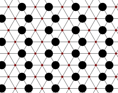
Deep inside the vortex condensate phase with in equation Eq. 6, the vector can have different condensates depending on the parameters in Eq. 26. Without loss of generality we set . The two figures in Eq. 4 illustrate the density waves of the bosonic parton centered at the bonds and the sites on the moiré triangular lattice that correspond to two different possible condensates of . The density on the bond is inferred from , with being the link on the dual honeycomb lattice that is dual to , and takes the sign according to the gauge convention of Fig. 1. The operator is the energy density in terms of vortex fields, and the modulation of this operator should correspond to the valence bond solid of the original bosonic parton. We also consider an operator centered on site of the original lattice (plaquette of the dual lattice): with the summation over the links that surround the plaquette on the dual honeycomb lattice, whose center hosts the site of the original moiré triangular lattice. In both cases, is evaluated using Eq. 42 and the value of which minimizes the quartic energy. The left pattern in Eq. 4 is a rather common valence bond solid configuration for either spin-1/2 system or hard core boson on the triangular lattice. If one started with the construction-I of the parton construction, the discussion in this section corresponds to the original electron system with an average 1/2 electron per unit cell (the filling considered in Ref. Jin et al. 2021); while for construction-II, the discussion here applies to one electron per unit cell, and the analysis in this section corresponds to one of the two spin/valley flavors of the system.
Appendix C Dual of the vortex theory
Here we derive the Lagrangian written in terms of the fractionally charged bosonic partons for scenario (1). We start with Eq. 6 in our paper:
| (59) |
To facilitate the calculation of the DC resistivity which will be discussed in the next subsection, we need to “dual back” to the charge-carriers, which requires deforming Eq. 59 with an easy-plane anisotropy . The bosonic fractional charge carriers are the vortices of the vortex fields . We first take the standard duality for , and Eq. 59 becomes:
| (60) |
The basic duality relation is that the current of , . Now integrating out would lead to the following constraint for the rest of the gauge fields:
| (61) |
From this constraint we can take as
| (62) |
Hence the dual of the dual theory becomes
| (63) |
The gauge fields are still subject to the constraint . carries charge of external EM gauge field; it also carries charge of gauge field which is shared with the fermionic parton .
For scenario (2) the theory in terms of fractional parton is much simpler: there is only one flavor of for each valley, and there is no extra continuous gauge fields besides gauge field : Following the calculation in Ref. Witczak-Krempa et al. 2012, one can generalize this one flavor of in each valley to an component of bosons:
| (64) |
and the bosons will scatter with both gauge field and field which is introduced as a Lagrange multiplier. The fact that carries charge of gauge field does not change the scattering rate through the large- calculation, as the gauge charge cancels out in the calculation of scattering rate through the large- approach. Compared with scenario (2), in scenario (1) the parton is also coupled to extra gauge fields , which will lead to extra scattering to the charge carriers.
When computing the resistivity, especially the DC resistivity of scenario (1), we also rely on a large generalization, namely we need to introduce an extra index for each component of fractional charge field: .
Appendix D DC resistivity jump in scenario (1)
In this section we present a detailed computation of the DC resistivity jump in the scenario (1) of MIT, i.e. the scenario when the insulator has a density wave. We start with Eq. 63. The resistivity jump at the MIT is given by the universal resistivity of the bosonic sector of the system at the MIT. First of all, one can prove a generalized Ioffe-Larkin rule, which combines the resistivity of each parton into :
| (65) |
where is the resistivity of each parton , when the charge of is taken to be 1. This generalized Ioffe-Larkin rule can be proven by formally integrating out , gauge fields and from Eq. 63, and eventually arriving at a response function of . At each level of the path integral, we keep a quadratic form of the action, i.e. the random phase approximation. This Ioffe-Larkin rule is independent of the assignment of electric charges on each parton.
To compute , we formulate the quantum Boltzmann equation (QBE) for the fields of a given valley. The computation follows that for at the MIT without charge fractionalization Witczak-Krempa et al. 2012, where the gauge field dynamics needs to be modified due to the charge fractionalization, which we explain in detail below for comparison. Note that can be finite without momentum relaxation due to the emergent particle-hole symmetry. Furthermore, the two-in two-out scatterings among the fields are enough to relax the current and generate finite DC resistivity. For simplicity, we consider the scattering between the and emergent gauge fields in Eq. (63), where the gauge fields are in thermal equilibrium and their dynamics is acquired due to the coupling with the matter fields and . Here, we argue that treating the gauge fields as in thermal equilibrium is a legitimate approximation. First, the gauge field couples to the spinon field , which is sensitive to impurities and relaxes momentum fast. Second, diagrammatically, the two-in two-out scatterings between the fields that give finite DC resistivity can be captured by the scattering with the emergent gauge fields.
To simplify the computation of the gauge field dynamics, it is convenient to express Eq. 63 in terms of the gauge field (Eq. 61), together with the effective action for the spinon field, the dual theory reads
| (66) |
Integrating out and fields, the gauge field propagators read
| (67) |
where is the current-current correlation function for and fields, respectively.
For a controlled systematic calculation of transport, we introduce a large number of (complex) rotor and spinon flavors with the constraint for all , and only the component couples to . The limit will be taken at the end. The effective action for the extended model becomes
| (68) |
Using the Fourier expansion for the electrically charged rotor in terms of the holons (+) and doublons (-),
| (69) |
the conductivity can be obtained as
| (70) |
where we define the distribution for holon () and doublon () as , and they satisfy the QBE as
| (71) |
Note that the gauge choice in Eq. 66 ensures that are decoupled and equal for different within the approximation that is in thermal equilibrium, so the subindex will be dropped unless there is ambiguity. The RHS of Eq. 71 reads
| (72) |
where and come from the bare vertex functions.
| 1 | 2 | 3 | 4 | 5 | 6 | … | ||
|---|---|---|---|---|---|---|---|---|
| 0.021 | 0.029 | 0.034 | 0.036 | 0.038 | 0.039 | 0.047 | ||
| 3.72 | 5.41 | 7.09 | 8.76 | 10.44 | 12.11 |
physically denote the density of states of the emergent fields that scatter with , which are broad in the space due to the couplings with the fields. Below, we ignore the bare dynamics. in the large- limit reads
| (73) |
where reduces to the MIT without charge fractionalization as discussed in Ref. Witczak-Krempa et al. 2012 when . For , as only the linear combination of , i.e. couples to the spinon field and is Landau damped, there is a factor for the Landau damped component of the gauge field propagator , which may also be understood as the component of gauge field in Eq. (63). The rest part is not Landau damped, and is determined solely by . Note that as in the limit , the Landau damped component can be approximated as , and be treated in the same way as Ref. Witczak-Krempa et al. 2012 for the gauge field . On the other hand, the first term in should be determined for generic . Using the standard expression for polarizations ,
| (74) |
Eq. (71) can be solved self-consistently. In Tab. 1, we show and the final resistivity at different , again the factor of arises from the two spin/valley flavors. increases roughly linearly with , and the fit of the data points at different gives
| (75) |