TSTG II: Projected Hartree-Fock Study of Twisted Symmetric Trilayer Graphene
Abstract
The Hamiltonian of the magic-angle twisted symmetric trilayer graphene (TSTG) can be decomposed into a TBG-like flat band Hamiltonian and a high-velocity Dirac fermion Hamiltonian. We use Hartree-Fock mean field approach to study the projected Coulomb interacting Hamiltonian of TSTG developed in Călugăru et al. [Phys. Rev. B 103, 195411 (2021)] at integer fillings and measured from charge neutrality. We study the phase diagram with , the ratio of and interlayer hoppings, and the displacement field, which introduces an interlayer potential and hybridizes the TBG-like bands with the Dirac bands. At small , we find the ground states at all fillings are in the same phases as the tensor products of a Dirac semimetal with the filling TBG insulator ground states, which are spin-valley polarized at , and fully (partially) intervalley coherent at () in the flat bands. An exception is with , which possibly become a metal with competing orders at small due to charge transfers between the Dirac and flat bands. At strong where the bandwidths exceed interactions, all the fillings enter a metal phase with small or zero valley polarization and intervalley coherence. Lastly, at intermediate , semimetal or insulator phases with zero intervalley coherence may arise for . Our results provide a simple picture for the electron interactions in TSTG systems, and reveal the connection between the TSTG and TBG ground states.
I Introduction
The rich physics discovered in twisted bilayer graphene (TBG), including the correlated insulating phase at integer fillings and the superconducting phase with finite doping have attracted the attention of both experimental and theoretical communities Lopes dos Santos et al. 2007; Suárez Morell et al. 2010; Bistritzer and MacDonald 2011; Cao et al. 2018a; Cao et al. 2018b; Cao et al. 2020a; Cao et al. 2020a; Chen et al. 2020; Liu et al. 2021a; Lu et al. 2019; Lu et al. 2021; Park et al. 2021a; Polshyn et al. 2019; Saito et al. 2020; Saito et al. 2021; Serlin et al. 2020; Stepanov et al. 2020; Wu et al. 2021a; Yankowitz et al. 2019; Choi et al. 2019; Choi et al. 2020; Kerelsky et al. 2019; Nuckolls et al. 2020; Wong et al. 2020; Xie et al. 2019; Jiang et al. 2019; Choi et al. 2021; Kang and Vafek 2019; Seo et al. 2019; Bultinck et al. 2020a; Hejazi et al. 2021; Fernandes and Fu 2021; Fernandes and Venderbos 2020; Venderbos and Fernandes 2018; Potasz et al. 2021; Abouelkomsan et al. 2020; Ahn et al. 2019; Bernevig et al. 2021a; Bernevig et al. 2021b; Bernevig et al. 2021c; Bultinck et al. 2020b; Cao et al. 2020b; Cea and Guinea 2020; Christos et al. 2020; Classen et al. 2019; Da Liao et al. 2019; Da Liao et al. 2021; Dai et al. 2016; Dodaro et al. 2018; Efimkin and MacDonald 2018; Eugenio and Dag 2020; González and Stauber 2019; Guinea and Walet 2018; Guo et al. 2018; Hejazi et al. 2019a; Hejazi et al. 2019b; Huang et al. 2019; Huang et al. 2020; Isobe et al. 2018; Jain et al. 2016; Julku et al. 2020; Kang and Vafek 2018; Kang and Vafek 2020; Kennes et al. 2018; Khalaf et al. 2021; König et al. 2020; Koshino et al. 2018; Ledwith et al. 2020; Lewandowski et al. 2021; Lian et al. 2019; Lian et al. 2021; Lian et al. 2020; Liu et al. 2012; Liu et al. 2018; Liu et al. 2019; Liu and Dai 2021; Liu et al. 2021b; Ochi et al. 2018; Padhi et al. 2020; Peltonen et al. 2018; Po et al. 2018; Po et al. 2019; Repellin et al. 2020; Repellin and Senthil 2020; Roy and Juričić 2019; Soejima et al. 2020; Song et al. 2019; Song et al. 2021; Tarnopolsky et al. 2019; Thomson et al. 2018; Uchida et al. 2014; Vafek and Kang 2020; Venderbos and Fernandes 2018; Wang et al. 2021; van Wijk et al. 2015; Wilson et al. 2020; Wu et al. 2018; Wu et al. 2019a; Wu et al. 2019b; Wu and Das Sarma 2020; Xie et al. 2020; Xie et al. 2021; Xie and MacDonald 2020a; Xie and MacDonald 2020b; Xu and Balents 2018; Xu et al. 2018; You and Vishwanath 2019; Yuan and Fu 2018; Zhang et al. 2020; Zou et al. 2018; Kwan et al. 2021; Zhang et al. 2021; Hofmann et al. 2021. The progress on TBG systems has also inspired interest in other twisted moiré materials. Among the twisted multilayer graphene systems and motivated by theoretical proposals in Refs. Suárez Morell et al. 2013; Khalaf et al. 2019; Mora et al. 2019; Li et al. 2019; Lopez-Bezanilla and Lado 2020; Carr et al. 2020; Park et al. 2020; Zhu et al. 2020; Lei et al. 2020; Wu et al. 2021b, the twisted symmetric trilayer graphene (TSTG) has recently been realized in experiments Hao et al. 2021; Park et al. 2021b; Cao et al. 2021. Correlated insulating states and superconducting states are also observed in TSTG. Similar to the twisted bilayer graphene, the electron density in TSTG is tunable via gate voltages. Moreover, an external displacement field perpendicular to the graphene sheets can be applied to the system, which makes the band structure also tunable by gate voltages. The experimental discoveries also triggered a deeper theoretical look at this system Călugăru et al. 2021; Shin et al. 2021; Fischer et al. 2021; Lake and Senthil 2021; Qin and MacDonald 2021; Chou et al. 2021.
TSTG is made of three graphene sheets in AAA stacking, with the middle layer twisted by a small angle relative to the top and bottom sheets. This lattice structure is shown to be energetically stable Carr et al. 2020. In the absence of the external displacement field, the system has mirror symmetry, by reflection around the graphene middle layer. Therefore we are able to use the eigenstates of this mirror symmetry as the basis: the TSTG decouples into two sectors with and mirror eigenvalues, which correspond to a TBG-like Hamiltonian with the effective interlayer hopping enhanced by a factor, and a Dirac cone Hamiltonian with a large unrenormalized Fermi velocity, respectively Khalaf et al. 2019. Similar to the pure TBG system, the TBG-like sector in TSTG exhibits flat bands at the TSTG magic angle , which is times of the TBG magic angle. The band dispersion also depends on the parameter , which is the ratio between interlayer in and hoppings. When an out-of-plane displacement field is turned on, these two mirror sectors will hybridize with each other. Equivalently, the out-of-plane displacement field can be captured by a interlayer potential . In Ref. Călugăru et al. 2021, we provided the perturbation schemes of the low energy bands in TSTG with and without the displacement field, derived the projected Hamiltonian for TSTG with a screened Coulomb interaction, and carefully analyzed the discrete symmetries and continuous symmetries of the TSTG Hamiltonian. These provide the foundation of the TSTG projected Hamiltonian we study in this paper.
In this paper, we employ the Hartree Fock (HF) mean field theory to study numerically the ground states of the projected interacting Hamiltonian of magic angle TSTG with a screened Coulomb repulsive interaction derived in Ref. Călugăru et al. 2021. We focus on integer fillings , defined as the number of electrons per moiré unit cell relative to the charge neutrality, where insulating or semimetallic behaviors are observed experimentally Hao et al. 2021; Park et al. 2021b; Cao et al. 2021. Our numerical results show that at small , the TSTG phases at all integer fillings are states that can adiabatically connect to the tensor product of a semimetal in the Dirac sector with the TBG sector ground states at flat band fillings : the TBG sector flat bands are fully spin-valley polarized at , fully intervalley coherent at and , and partially intervalley coherent at . The only exception is the case of with , where the TSTG may enter a large Fermi surface metal phase with competing orders, including a potential translation symmetry breaking, due to the charge transfers between the Dirac and TBG sectors. At fillings , as increases (at ), we find a universal first order transition into a phase with zero intervalley coherence, which either remains a semimetal () or may even become an insulator (). Lastly, at stronger for which the TSTG free bandwidth exceeds the Coulomb interaction energy scale, all the integer fillings enter a metallic phase with large Fermi surfaces and small or zero valley polarization and intervalley coherence.
The rest of the paper is organized as follows. In Sec. II, we review the single body Hamiltonian of TSTG and its mirror symmetric basis. The projected Hamiltonian into the low energy bands being studied is also discussed. Sec. III presents the Hartree-Fock mean field approximation to the TSTG projected Hamiltonian, the self consistent conditions, and the HF order parameters which characterize the physical properties of the mean field ground state. In Sec. IV, we provide the HF numerical results at integer filling factor . The phase diagram and ground state properties are discussed. We have also calculated the HF band structure in different phases. Similarly, the discussion of the HF numerical results at filling factors and are also presented in Secs. V, VI and VII, respectively.
II Interacting Model for TSTG
We first briefly review the non-interacting Bistritzer-MacDonald Hamiltonian for mirror symmetric twisted trilayer graphene, which can be written as the sum of a TBG Hamiltonian Bistritzer and MacDonald 2011 with renormalized interlayer hopping and an independent Dirac fermion Hamiltonian Khalaf et al. 2019; Călugăru et al. 2021. We also introduce a displacement field perpendicular to the graphene sheets that can couple the Dirac fermion and TBG fermion together. The interacting Hamiltonian projected into the low energy bands is also discussed in this section Călugăru et al. 2021.
II.1 Single particle Hamiltonian
The twisted trilayer graphene geometry with mirror symmetry was introduced in Refs. Khalaf et al. 2019; Mora et al. 2019. In this article we will use the notations of Ref. Călugăru et al. 2021; Bernevig et al. 2021a; Bernevig et al. 2021b; Bernevig et al. 2021c; Lian et al. 2021; Song et al. 2019; Song et al. 2021; Xie et al. 2021 where the non-interacting model and its symmetries are discussed in detail. We use to represent the electron creation operator with momentum measured from the point of single layer graphene Brillouin zone, sublattice , spin and layer . Similar to the derivation of Bistritzer-MacDonald model for twisted bilayer graphene, Dirac equation can be used to describe the low energy physics of each individual layer. We define as the point of the bottom and the top layers, and for the middle layer. Here . For convenience, we also define vectors . The reciprocal lattice of the moiré lattice is spanned by the basis vectors and . Adding the vectors iteratively gives us momentum lattices , and they form the hexagon lattice in the momentum space. In order to describe the low energy physics, we introduce the electron operators , where if or if . Without the displacement field along direction, the system is invariant under mirror symmetry which switches the first layer with the third layer, and leaves the middle layer invariant. Therefore, the Bistritzer-MacDonald model for TSTG can be simplified using the following basis transformation:
where belongs to the moiré Brillouin zone (MBZ). These operators (dubbed as TBG fermions) have even eigenvalue under transformation. Fermion operators with odd eigenvalue (dubbed as Dirac fermions) are given by:
| (3) |
Since the single body Hamiltonian commutes with transformation in the absence of the external displacement field, it can be written as a block diagonal form:
| (4) |
It can be shown that the Hamiltonian in the mirror symmetric sector contains operators and is identical to the ordinary TBG Hamiltonian Bistritzer and MacDonald 2011; Song et al. 2019, with the interlayer hopping parameter multiplied by a factor of . It reads:
| (5) |
in which the “first quantized Hamiltonian” of the valley is given by:
| (6) |
where is the Fermi velocity of single layer graphene, and interlayer hopping matrices are given by:
| (7) |
Similar to the TBG Hamiltonian, and stand for the interlayer hopping strength around the and stacking regions, respectively. In this article we use as a tunable parameter, and keep the value of fixed. Similar to ordinary TBG, we define as the chiral limit. In the realistic case we have due to lattice relaxation effects Uchida et al. 2014; van Wijk et al. 2015; Jain et al. 2016; Koshino et al. 2018. The factor in Eq. (6) comes from the transformation in Eq. (II.1). Due to the fact that the effective interlayer hopping is stronger, the magic angle of TSTG where the bands around charge neutral point are flat will be around , which is bigger than the magic angle in TBG Khalaf et al. 2019. The Hamiltonian in valley can be obtained by applying transformation to Eq. (6).
On the other hand, only includes the contribution from mirror anti-symmetric sector. It is given by the following expression:
| (8) |
in which the first quantized Hamiltonian for Dirac cone reads:
| (9) | ||||
| (10) |
We can introduce an external displacement field perpendicular to the graphene sheets. When this external field is turned on, the mirror symmetry is broken, which will lead to mixing terms between the TBG fermions in the mirror symmetric sector and the Dirac fermions in the mirror anti-symmetric sector. We denote the potential difference between the top and bottom layer by , and the Hamiltonian which describes the electric field can be written as:
| (11) |
This Hamiltonian can be rewritten using the Dirac and TBG fermions:
| (12) |
which couples the mirror symmetric and anti-symmetric sectors. In conclusion, the non-interacting Hamiltonian can be written as the summation of these three terms:
| (13) |
II.2 Interaction and Projected Hamiltonian
In this article we will assume that the interaction between electrons in TSTG system is given by the Coulomb potential screened by a top and bottom gate. The interaction Fourier transformation reads:
| (14) |
where is the distance between the top and bottom gates, and is the strength of the Coulomb interaction with dielectric constant Cao et al. 2018a; Cao et al. 2018b; Kang and Vafek 2018. The interacting Hamiltonian can be written as Kang and Vafek 2019; Bernevig et al. 2021b; Călugăru et al. 2021:
| (15) |
where is the area of moiré unit cell, and is the number of moiré unit cells. is the electron density at momentum relative to the charge neutral point and can be written as:
| (16) | ||||
| (17) | ||||
| (18) |
By projecting the system into the low energy bands, the dimension of Hamiltonian matrix in Hartree Fock calculation will be reduced dramatically, and therefore greatly improving the numerical calculations. By diagonalizing the single particle TBG Hamiltonian and the Dirac Hamiltonian , we obtain the dispersion relation and the single body wavefunctions for the TBG and Dirac fermions (). For each spin and valley, we project the kinetic Hamiltonian into the two bands which are closest to the charge neutral point for both and . Therefore, the kinetic part of the projected Hamiltonian can be written in the following form when :
| (19) |
where the creation operators in band indices are defined as . The Dirac fermions in the antisymmetric sector are degenerate on certain high symmetry lines between the projected bands and the bands above and below when folding over the MBZ, therefore there is an ambiguity of choosing its single-body wavefunction. We provide a careful discussion of this issue and how we solve it in Appendix A.
As shown in Refs. Bultinck et al. 2020a; Hejazi et al. 2021; Bernevig et al. 2021b; Lian et al. 2021, by fixing the sewing matrix of symmetry to identity (where is the 2-fold rotation about the axis, and is the time reversal), one can recombine the TBG flat energy band basis into a Chern band basis
| (20) |
where gives the Chern number of the Chern band basis (which is also the eigenvalue of the Pauli matrix in the space of TBG energy band index ).
The displacement field term in Eq. (12) can also be written using band basis and projected into the lowest bands:
| (21) |
where the displacement field overlap matrices are given by
| (22) |
Thus the projected non-interacting Hamiltonian can be written as the following quadratic form:
| (23) |
in which the matrix is given by
| (24) |
Here is the dispersion of TBG() and Dirac() fermions without displacement field. The eigenvalues of can give us the approximate dispersion of the non-interacting TSTG at non-zero displacement field. The projected Hamiltonian can capture the band width of the bands around charge neutrality accurately Călugăru et al. 2021. We also provide plots comparing the dispersion of the projected Hamiltonian and the band structure obtained from the unprojected BM Hamiltonian in Appendix A Fig. S2 Călugăru et al. 2021.
Similarly, the interacting Hamiltonian can also be projected into these bands:
| (25) |
in which the density operators after being projected are defined as:
| (26) | ||||
| (27) | ||||
| (28) |
The components of these form factors depend on the gauge choice of the single body wavefunctions. As mentioned in Eq. (20), we fix the gauge choice of the single-body wavefunction of the TBG fermions such that the sewing matrix of is the identity.
For convenience, we can rewrite the interacting Hamiltonian as the following form:
| (29) |
in which the matrix elements are given by:
| (30) |
The mean field Hamiltonian will have a simpler form using this notation, as we will discuss in Sec. III.
In this paper, we fix the twist angle to , which is near the magic angle of TSTG and gives rise to flat bands in the mirror symmetric sector. Since both the band structure and the wavefunctions of the mirror symmetric sector depend on the parameter , the projected Hamiltonian also depends on . And by adding all the terms in kinetic energy and potential energy, we obtain the tunable Hamiltonian with parameters and :
| (31) |
Similar to that in TBG, we define as the chiral limit, and (zero TBG bandwidth) as the flat (TBG band) limit. In these limits or their combinations, the symmetry of the TSTG is enhanced to a symmetry in the combined spin and valley space Călugăru et al. 2021. In this paper, we will not tune the bandwidth in the mirror symmetric (TBG) sector, therefore the non-interacting band structure will only depend on and (at the fixed twist angle and AB/BA interlayer hopping strength ).
III Hartree-Fock Theory
We perform Hartree Fock (HF) mean field calculations for the projected Hamiltonian we obtained in Eq. (31), which is at fixed twist angle . In Appendix B, we provide a more detailed discussion of the HF calculations. In this section, we focus on the assumption and the quantities that we will rely on in the rest of our paper.
In Refs. Kang and Vafek 2018; Zhang et al. 2020; Bultinck et al. 2020a; Lian et al. 2021; Xie et al. 2021, it has been shown that the ground states of TBG at integer fillings (integer number of electrons per moiré unit cell, relative to the charge neutral point) around the chiral flat band limit (i.e. the value of is small and disregarding the flat band dispersion) are correlated insulator states (sometimes with non-zero Chern number) without translation symmetry breaking. This picture is expected to be valid till reasonably large physical values (depending on electron fillings) Kang and Vafek 2020; Soejima et al. 2020; Xie et al. 2021. Meanwhile, the high Fermi velocity and vanishing Fermi surfaces of the Dirac fermions make them unlikely to contribute to translation symmetry breaking (which requires certain low energy Fermi surface nestings).
Therefore, we assume there is no translation symmetry breaking in our HF calculation for TSTG (with a notable exception in 1 where we discuss the possible CDW order at point at filling). This assumption simplifies our numerical calculation by reducing the number of HF mean field order parameters. For this reason, within the assumption, the HF mean field order parameter can be defined as the following matrix at each :
| (32) |
where stand for the TBG and Dirac fermion operators. The matrix is the single-body density matrix at each momentum . As we explained, this assumption of no translation breaking is reasonable when is small (typically ), and it is possible that our assumption will be violated for large Kang and Vafek 2018; Xie et al. 2021. Therefore, the Hartree Fock result is less trustable when gets bigger.
For an arbitrary momentum , the Hartree and Fock mean field Hamiltonians are given by the following:
| (33) | ||||
| (34) |
Together with the non-interacting term defined in Eqs. (23) and (24), we obtain the Hartree Fock Hamiltonian . By diagonalizing the Hartree Fock Hamiltonian, we obtain the HF band structure , which is related to the dispersion of the charge excitations, and the corresponding wavefunction :
| (35) |
For a filling factor , which is defined as the number of electrons per moiré unit cell relative to charge neutrality, the HF ground state is given by occupying the single particle states (where at each ) from low to high up to filling . For each single body state , valley polarization can be defined as:
| (36) |
and the valley physics of the system can be captured by of each individual occupied state at every .
The self-consistent condition also gives a relation between these wavefunctions and the order parameter:
| (37) |
For each integer filling factor , we use various initial conditions in our HF calculation, and we choose the result with the lowest energy. Detailed discussion about the choices of initial conditions at different filling factors can be found in Appendix B. In this article, the filling factor is measured from the charge neutrality, and it is related with the order parameter in Eq. (37) by:
| (38) |
Moreover, since the particle numbers of Dirac fermion and TBG fermion are conserved when the displacement field is turned off, we can define the filling factors (measured from the charge neutrality) for these fermion flavors separately:
| (39) | ||||
| (40) |
The summation of these two quantities is the total filling factor:
| (41) |
For the projected bands we keep, the two filling factors range within and , respectively. We will be focusing on total integer fillings in this paper. Since the physics at filling is particle-hole symmetric to that at filling Călugăru et al. 2021, it is sufficient to study fillings .
Various physical quantities can be derived from , which can be used to describe the nature of the ground state, such as the intervalley coherence and valley polarization. As shown in Ref. Lian et al. 2021, the ground state at filling in TBG has intervalley coherence when the system is non-chiral non-flat. In order to measure the coherence between the two valleys, we define the quantity which is based on the norm of the off-diagonal block in valley space:
| (42) |
where is the number of moiré lattice sites. This quantity includes both the contribution from the TBG flat bands and the Dirac fermions. Its value is
| (43) |
if there are filled TBG flat bands which are fully intervalley coherent.
The expectation value of any single-body quantity can be obtained from the Hartree-Fock order parameter . In this article, we calculate three quantities that we will now define: the valley polarization , the spins in each valley and the quantity which provides information about the Chern number of the occupied TBG fermions.
The valley polarization is the electron number difference between the two valleys. This can also be obtained from the order parameter:
| (44) |
where is the Pauli matrix in valley space.
Similarly, we can track the spin order. Due to the U(2)U(2) symmetry of the system, the total spin of the two valleys are conserved independently. For each valley , the semi-classical total spin per moiré unit cell can be obtained by the following equation:
| (45) |
where are the Pauli matrices in spin space.
Finally, we can define a quantity within the TBG band sector:
| (46) |
where is the Pauli matrix in the space of the energy band index . If the Dirac bands and the TBG bands in the HF Hamiltonian are decoupled (e.g. at and without breaking order parameters), characterizes the Chern number in the TBG sector when the TBG sector is insulating, which can be seen by transforming into the Chern band basis in Eq. (20). Generically (e.g., ), is not necessarily an integer, but it is related with the Chern number of the (partially or fully) occupied TBG flat band basis. For example, this value is close to if the two occupied TBG flat bands have the same Chern number. Similar to the filling factor for Dirac and TBG fermion flavors, this quantity is a useful characterization of the many-body state when is close to zero.
We perform the HF calculations on a preserving momentum lattice in the MBZ (see Fig. S1), with up to . As discussed in Appendix B, we are also able to obtain the band structure plot along high symmetry lines by using the HF order parameters we obtained on these lattices. In the band structure plots, we use subscript to denote the high symmetry points in the moiré Brillouin zone. Our HF calculations are restricted within the pamameter ranges and . We do not discuss the HF calculation in the chiral limit in this paper, the convergence of which is difficult due to the enhanced symmetry and enlarged ground state degeneracy manifold. We note that the realistic TSTG is always away from the chiral limit.
IV Numerical Results at filling factor


We start our discussion about HF calculations for TSTG with filling factor . As a comparison, the ground state at filling in TBG at small and small nonzero bandwidth is a spin and valley polarized Chern insulator state with Chern number , and may enter translation or rotation symmetry breaking phases at large , which has been predicted in Refs. Zhang et al. 2020; Bultinck et al. 2020a; Lian et al. 2021; Xie et al. 2021. In this section, we will explore the HF ground states in TSTG at in the parameter space of and (see Eq. (31) for definition).
Here we restrict the parameter ranges within and . The maximal value of is motivated by the experimental results Park et al. 2021b. The valley polarization as a function of and is shown in Fig. 1(a). We find the HF ground states show different behaviors in three different parameter regions, which are labeled by I, II and III in Fig. 1(a). We also calculate other physical quantities, including and , the values of which along certain line cuts in the parameter space are shown in Fig. 1(b) and (c). Based on these quantities, we describe the TSTG phases in the three regions in details below.
Region I: we find and throughout the whole region (Fig. 1(b) and (c)). This indicates that the ground state is a spin-valley polarized state dominantly occupying one Chern band in the TBG sector (defined in Eq. (20)) of a particular spin and valley. In particular, at , where the electron numbers in the Dirac sector and the TBG sector are both conserved, we find and within region I (see in Fig. 1(d)). Therefore, in region I, the HF ground state at is the tensor product of the TBG spin-valley polarized Chern insulator and the Dirac fermion semimetal at charge neutrality . The ground states at in region I are adiabatically in the same semimetal phase. As an example, the band structure at and is shown in Fig. 2(a), which is almost a Dirac semimetal. At , where the Dirac and TBG sectors are hybridized, the gapless Dirac nodes are due to the symmetry within the empty valley-spin flavors, as shown in Appendix D. The color (from red to purple) indicates the valley polarization of of each band, and an occupied flat band can be seen clearly.
Region II: we find the valley polarization drops abruptly to small values near zero, and so do the other quantities as shown in Fig. 1(b) in this region where the displacement field is large. Accordingly, the HF ground state can be understood as a metal with little spin/valley polarization or intervalley coherence. A typical HF band structure in region II is shown in Fig. 2(b), which has a large Fermi surface around () point in valley (), showing that the system is a metal. A sharp phase boundary between region I and II can be identified in Fig. 1(a), which is at when , and at when . The reason for such a metallic phase is that a large significantly hybridizes the Dirac sector and the TBG sector, and turns the flat bands near () point of valley () into dispersive Dirac fermions with kinetic energies comparable to the interaction energies. This leads to a Fermi surface reconstruction, where electrons prefer to occupy the electron states near the and points with lower kinetic energies and form a metal. We provide the non-interacting band width as a function of and in Figs. S4(a) and (b) of Appendix A. The phase boundary between region I and II is close to an equal value contour in these figures, which also implies that the transition to the metallic phase happens as the non-interacting bandwidth exceeds a critical value around the order of the interaction energy scale.
Region III: we find that the HF ground state exhibit competing orders in this region which is located in the weak displacement field region with . In Fig. 1(c) we plot the HF mean field quantities, e.g. , and , at with respect to . When (region III), we see all the quantities are strongly oscillating. Moreover, we also notice strong size effect in this region, which can be seen by considering other system sizes at , as discussed in Appendix C. In previous numerical studies in TBG systems Kang and Vafek 2020; Soejima et al. 2020; Xie et al. 2021 (which do not have the parameter), it has been shown that the translation symmetry of the TBG at filling could be broken at large (typically ). Therefore, we expect the ground states in region III not to be accurately captured by our HF calculation, which does not allow translation symmetry breaking. In 1, we provide numerical evidence for a translation symmetry breaking phase via a modified HF calculation. Nevertheless, we provide some universal observation of our HF results in region III. In Fig. 1(d), we plot and as a function of at . We find the Dirac electron filling is for (i.e., in region I), but begins to decrease as increases beyond (i.e., in region III). This indicates that electrons are transferred from the Dirac valence bands into the TBG flat bands in region III, making and . For instance, when at , our HF calculation shows that and , the HF band structure of which is shown in Fig. 2(c). The Fermi level of this HF band structure in region III is far from the Dirac point energy, giving rise to a metal with large Fermi surfaces. Therefore, the ground states in region III are likely to be metals with competing orders, such as translation symmetry breaking.
In summary, at , we have identified three phases in three regions of Fig. 1(a). In region I the ground state is almost a spin-valley polarized semimetal, in region II the ground state is a metal with little spin/valley polarization or intervalley coherence, while in region III the ground state may be a metal with competing orders.
V Numerical Results at filling factor
In this section, we study the HF results for TSTG at integer filling . By comparison, in TBG systems, the ground state at at small and small bandwidth is given by an intervalley coherent insulator with Chern number , which has been predicted in Refs. Kang and Vafek 2018; Bultinck et al. 2020a; Zhang et al. 2020; Lian et al. 2021; Xie et al. 2021. At large , the TBG ground state may become a metal Bernevig et al. 2021c. However, there is no evidence of translation symmetry breaking at in TBG so far. Therefore, we also conjecture that translation breaking is less likely in the TSTG at , and thus regard our HF results as more reliable than at in the large region.
Our HF results for TSTG at identified 3 distinct regions I, II, III in the and parameter space as shown in Fig. 3(a). In Fig. 3(a), the color scale indicates the ground state intervalley coherence , defined in Eq. (42) (note that this is different from the phase diagram Fig. 1(a), where valley polarization is shown by color, while intervalley coherence is near zero). Other HF quantities along certain constant line cuts are shown in Fig. 3(b) and (c). From these quantities, we can see clear phase transitions between regions I and II, and between regions II and III. We now describe the HF ground states in the three regions, respectively.


Region I: this region contains the entire range of up to some -dependent value. There we find , , and . This implies that there are two fully intervalley coherent flat bands occupied, which have the same spin and have zero total Chern number. This is the same as the TBG ground state at filling. When in region I, the electron numbers in the Dirac sector and the TBG sector are conserved, respectively, and the HF ground state is almost the tensor product of the intervalley coherent TBG ground state predicted in Refs. Kang and Vafek 2018; Bultinck et al. 2020a; Zhang et al. 2020; Lian et al. 2021; Xie et al. 2021 and the Dirac band ground state at charge neutrality . A typical band structure in region I at and is given in Fig. 4(a), where the valley polarization values of the occupied single body states (defined in Eq. (36)) are represented by color. One can see the valley polarization of the 2 occupied flat bands are approximately zero, consistent with an intervalley coherent state. The ground state in region I is thus almost an intervalley coherent semimetal, in which the Dirac fermion is slightly doped away from the Dirac nodes. In particular, at where the Dirac and TBG sectors are hybridized, the gapless Dirac nodes are protected by a remaining anti-unitary symmetry (), which is a combination of the and a relative intervalley phase rotation (see Appendix D).
Region II: the interlayer potential is intermediate, and we find and . This indicates that the ground state becomes a valley polarized state, and the two occupied TBG flat bands approximately have zero total Chern number. We plot two typical HF band structures with different values in Fig. 4(b) and (c). In both of the band structure plots, the valley polarization values of occupied single body states in the flat bands are . The occupied flat bands with smaller (larger) value has smaller (larger) band width. The band structures plots also show that there is a small electron pocket around point, and a small hole pocket around point, indicating the system is almost a semimetal with a small Fermi surface.
Region III: the interlayer potential is further increased (e.g., at , and at ), the valley polarization drops significantly, and the intervalley coherence slightly re-enters, as shown in Fig. 3(b) and (c). In this case, the TSTG enters a metallic phase with large Fermi surfaces. A HF band structure in this region is shown in Fig. 4(c). Similar to the region II phase at filling , the region III phase at here is due to the change of flat bands into high energy dispersive Dirac bands near () point of valley () at large , yielding transitions into less valley polarized metal with large Fermi surfaces.
To summarize, the phase diagram at filling factor can be roughly separated into three regions, as shown in Fig. 3(a). In the small region I, the ground state is nearly an intervalley coherent semimetal and is adiabatically connected with the tensor product of the TBG ground state and a high velocity Dirac fermion at charge neutrality. In region II with intermediate , the ground state is fully valley polarized and almost a semimetal. Finally, in region III with large , the system enters a metal phase with partial valley polarization.
VI Numerical Results at filling factor
In this section, we discuss the HF calculation results for TSTG at filling factor . We first recall that the ground state at in nonchiral-nonflat TBG systems carries a Chern number and has two intervalley coherent bands and one valley polarized band occupied, as shown in Refs. Lian et al. 2021; Zhang et al. 2020. Similar to filling and , we expect the TSTG ground state at small and to be the tensor product of the TBG ground state at this filling and the half filled Dirac fermion bands.
The intervalley coherence of the TSTG HF ground state at as a function of and is represented by the color code in Fig. 5(a). Other HF quantities at and are shown in Figs. 5(b) and (c), respectively. Based on these quantities and the HF band structures, we are able to identify four different regions I, II, III and IV in and parameter space as shown in Fig. 5(a). We now describe the HF mean field results in these regions.


Region I: this region encompasses the entire range of , and up to certain -dependent value, and we find that , , , and . The value of intervalley coherence indicates that among the three occupied TBG flat bands, two of them are intervalley coherent. These values also imply that the HF ground state at is approximately equal to the tensor product of a intervalley coherent state Zhang et al. 2020; Lian et al. 2021 and a half-filled Dirac semimetal. Fig. 6(a) shows a typical HF band structure in region I at and . Among the three occupied flat bands in Fig. 6(a), two of them have zero valley polarization, while the other one is valley polarized, which agrees with the expected ground state in the TBG sector. The ground states of region I is adiabatically connected to the ground state. Therefore, region I is a semimetal phase with partially intervalley coherent flat bands. Similar to the case, the gapless Dirac nodes at are protected by the symmetry within an empty valley-spin flavor, as shown in Appendix D.
Region II: the displacement field is intermediate in this region (e.g. at , or at ). We find that the values of HF quantities , and are close to their values in region I. However, the intervalley coherence vanishes abruptly in this region. We present a HF band structure at and in Fig. 6(b). The valley polarization of the three occupied flat bands are . The band structure also shows small electron pocket around point, and hole pocket around point, which means the system is also almost a semimetal without intervalley coherence.
Region III: the displacement field in this region (which is at ) is stronger than that in the region II. We find the valley polarization drops to zero, and the intervalley coherence slightly increases to , as shown in Fig. 5(b). The HF band structure in this region, which can be found in Fig. 6(c), shows that there is a direct band gap around the Fermi level. Therefore, we identify an insulating state at filling with a non-zero displacement field in region III. Such a phase does not occur at or fillings.
Region IV: the displacement field is further increased (e.g., at ). Similar to the strong field phase at and , the increased bandwidth of the non-interacting dispersion becomes comparable to or larger than the strength of the Coulomb interaction. Therefore, the electrons will first occupy the low energy states around and at which can be seen in Fig. 6(d). A large Fermi surface can also be observed in the band structure, which implies that region IV is a metallic phase. Both the valley polarization and the intervalley coherence are nearly zero in this region.
In summary, there are four phases in the phase diagram at filling factor . When the displacement field is close to zero, i.e., in region I, the ground state is an intervalley coherent semimetal. As the displacement field increases into region II, the ground state becomes a semimetal without intervalley coherence. When the field further increases into region III, the HF band structure becomes gapped, and therefore the ground state is an insulator. We note that this phase does not occur at fillings and . Finally in region IV with the strongest displacement field, the system becomes a metal, similar to the filling factors and .
VII Numerical Results at filling factor
Lastly, we present our HF calculation results for TSTG at filling factor . In comparison, in the TBG system the ground state at is an insulator state with four occupied intervalley coherent bands and zero total Chern number Zhang et al. 2020; Lian et al. 2021. Similar to other integer fillings, we expect the ground state of TSTG at and to be the tensor product of a TBG intervalley coherent insulator ground state and half filled Dirac semimetal.


In Fig. 7(a), we show the intervalley coherence in the and parameter space at . By using the same method as the HF band structure along the high symmetry lines, which is discussed in 2, we can estimate the HF Hamiltonian at any momenta not included in the momentum lattice employed in our HF iterations. Thus, the energy gap around the Fermi level along the high symmetry lines as a function of and can be calculated, which is shown in Fig. 7(b). We are able to identify three different regions I, II and III in the and parameter space, based on the valley coherence and the energy gap. Other HF quantities at fixed and are also shown in Figs. 7(c) and (d). We now use these quantities to describe the HF ground states in these regions.
Region I: this region is in the low displacement field regime, and we find the values of the HF quantities are , , and . The value of the intervalley coherence shows that there are four occupied intervalley coherent bands and have zero total Chern number. Therefore, these values indicates that the HF ground state at can be well approximated by the tensor product of the insulating intervalley coherent TBG ground state at predicted in Refs. Zhang et al. 2020; Lian et al. 2021, and the ground state at in region I is adiabatically connected to this tensor product state. A typical HF band structure can be found in Fig. 8(a). The occupied flat bands have zero valley polarization, which agree with the intervalley coherent ground state. Therefore, the TSTG ground state is an intervalley coherent semimetal. As we show in Appendix D, the gapless Dirac nodes of this phase at is protected by a remaining anti-unitary symmetry (), which is a combination of the and a relative phase rotation between the two valleys.
Region II: the displacement field is intermediate, and as seen in both Figs. 7(b) and (c), the intervalley coherence drops to zero in this region. Other HF parameters, including , and are equal to zero in region II. We also notice that there is another state with non-zero values in region II, whose energy increment from the state with is within the machine precision when the parameters are around the boundary between regions II and III, showing a possible competing order. A typical HF ground state band structure in region II is shown in Fig. 8(b). The occupied flat bands have valley polarization values , and there is a large direct gap around the Fermi level. This result indicates that region II is an insulating phase, akin to the region III at filling.
Region III: here the interlayer potential is stronger, and the HF quantities , , and in this large region are the same as in region II. However, the band structures undergo an abrupt transition. As discussed in previous sections, the bandwidth of the low energy bands become large when is large, and therefore the effect of the interaction will be suppressed by the kinetic energy. A HF band structure in this region is shown in Fig. 8(c). The HF mean field band structure is similar to the non-interacting band dispersion, which has gapless Dirac points at and points. The discontinuous dispersions in Fig. 8(c) at and (see the zoom-in plots in Fig. 8(c)) are due to neglecting of the higher bands in the TSTG projected Hamiltonian, as explained in Appendix A. From the HF band structure, we conclude that the large displacement field phase in region III at filling becomes a semimetal.
To summarize, there are three phases at filling factor , as shown in Fig. 7(b). Within the small region I, the HF ground state is an intervalley coherent semimetal. In region II with an intermediate , the ground state is an insulator without intervalley coherence or valley polarization. Finally, in region III with a large , the system becomes a semimetal with no valley polarization or intervalley coherence.
VIII Conclusion
Through projected Hartree-Fock mean field calculations, our work unveiled the close relationship between TSTG at weak displacement field and TBG systems at integer fillings and . We show that at weak displacement fields, the TSTG ground states at integer fillings are almost semimetal states which are in the same phase as the tensor product of the TBG ground states at the same filling and a Dirac semimetal. Beyond the phases inherited from the TBG physics, the TSTG undergoes transitions into large Fermi surface metals or insulators as the displacement field increases. Besides, we generically find that the displacement field destabilizes the intervalley coherence of the flat bands.
For filling factor , we found three regions of different phases. At small displacement field, the TSTG ground state is a semimetal with an occupied spin-valley polarized flat band when . At large displacement fields, the TSTG undergoes a first order phase transition into a metallic phase with large Fermi surfaces and zero valley polarization, due to the enlarged band width. When and , we observed that the electrons transfer from the Dirac cones into the TBG flat bands, which yields a metallic phase with competing orders. Moreover, similar to pure TBG systems at , it is possible to have translation symmetry breaking, some evidence of which is shown in 1. We leave the study of translation breaking TSTG phases in the future.
For filling factors and , our HF numerical results show that the TSTG ground states at weak displacement fields are semimetals with intervalley coherent flat bands occupied. At intermediate displacement fields, the intervalley coherence drops abruptly to zero, signaling a transition into phases without intervalley coherence, which are either semimetals (at and ) or insulators (at and ). With a stronger displacement field, the dispersive energy bands will have bandwidths exceeding the energy scale of Coulomb interactions, which leads the system into a metallic state with little valley polarization or intervalley coherence.
Our work reveals two roles of the displacement field in TSTG with Coulomb interaction: destabilizing the intervalley coherence (if any), and increasing the flat band width and thus weakening the correlations due to interactions. Our results may provide guidance to the analytical studies of TSTG ground states in the future.
Acknowledgements.
We are grateful to Zhi-Da Song for previous collaboration on related works and enlightening discussions. We thank Oskar Vafek, Pablo Jarillo-Herrero, and Dmitri Efetov for fruitful discussions. This work was supported primarily by the ONR No. N00014-20-1-2303, the Schmidt Fund for Innovative Research, Simons Investigator Grant No. 404513, the Packard Foundation, the Gordon and Betty Moore Foundation through Grant No. GBMF8685 towards the Princeton theory program, and a Guggenheim Fellowship from the John Simon Guggenheim Memorial Foundation. Further support was provided by the NSF-EAGER No. DMR 1643312, NSF-MRSEC No. DMR-1420541 and DMR-2011750, DOE Grant No. DE-SC0016239 , Gordon and Betty Moore Foundation through Grant GBMF8685 towards the Princeton theory program, BSF Israel US foundation No. 2018226, and the Princeton Global Network Funds. B.L. acknowledges support from the Alfred P. Sloan Foundation.Note added.—During the final preparation of this manuscript, a recent preprint Ref. Christos et al. 2021 appeared, with numerical results consistent with ours at even integer fillings.
References
- Lopes dos Santos et al. (2007) J. M. B. Lopes dos Santos, N. M. R. Peres, and A. H. Castro Neto, Phys. Rev. Lett. 99, 256802 (2007).
- Suárez Morell et al. (2010) E. Suárez Morell, J. D. Correa, P. Vargas, M. Pacheco, and Z. Barticevic, Phys. Rev. B 82, 121407 (2010).
- Bistritzer and MacDonald (2011) R. Bistritzer and A. H. MacDonald, PNAS 108, 12233 (2011).
- Cao et al. (2018a) Y. Cao, V. Fatemi, A. Demir, S. Fang, S. L. Tomarken, J. Y. Luo, J. D. Sanchez-Yamagishi, K. Watanabe, T. Taniguchi, E. Kaxiras, R. C. Ashoori, and P. Jarillo-Herrero, Nature 556, 80 (2018a).
- Cao et al. (2018b) Y. Cao, V. Fatemi, S. Fang, K. Watanabe, T. Taniguchi, E. Kaxiras, and P. Jarillo-Herrero, Nature 556, 43 (2018b).
- Cao et al. (2020a) Y. Cao, D. Chowdhury, D. Rodan-Legrain, O. Rubies-Bigorda, K. Watanabe, T. Taniguchi, T. Senthil, and P. Jarillo-Herrero, Phys. Rev. Lett. 124, 076801 (2020a).
- Chen et al. (2020) G. Chen, A. L. Sharpe, E. J. Fox, Y.-H. Zhang, S. Wang, L. Jiang, B. Lyu, H. Li, K. Watanabe, T. Taniguchi, Z. Shi, T. Senthil, D. Goldhaber-Gordon, Y. Zhang, and F. Wang, Nature 579, 56 (2020).
- Liu et al. (2021a) X. Liu, Z. Wang, K. Watanabe, T. Taniguchi, O. Vafek, and J. I. A. Li, Science 371, 1261 (2021a), https://science.sciencemag.org/content/371/6535/1261.full.pdf .
- Lu et al. (2019) X. Lu, P. Stepanov, W. Yang, M. Xie, M. A. Aamir, I. Das, C. Urgell, K. Watanabe, T. Taniguchi, G. Zhang, A. Bachtold, A. H. MacDonald, and D. K. Efetov, Nature 574, 653 (2019).
- Lu et al. (2021) X. Lu, B. Lian, G. Chaudhary, B. A. Piot, G. Romagnoli, K. Watanabe, T. Taniguchi, M. Poggio, A. H. MacDonald, B. A. Bernevig, and D. K. Efetov, Proceedings of the National Academy of Sciences 118, 10.1073/pnas.2100006118 (2021), https://www.pnas.org/content/118/30/e2100006118.full.pdf .
- Park et al. (2021a) J. M. Park, Y. Cao, K. Watanabe, T. Taniguchi, and P. Jarillo-Herrero, Nature 592, 43 (2021a).
- Polshyn et al. (2019) H. Polshyn, M. Yankowitz, S. Chen, Y. Zhang, K. Watanabe, T. Taniguchi, C. R. Dean, and A. F. Young, Nat. Phys. 15, 1011 (2019).
- Saito et al. (2020) Y. Saito, J. Ge, K. Watanabe, T. Taniguchi, and A. F. Young, Nat. Phys. 16, 926 (2020).
- Saito et al. (2021) Y. Saito, J. Ge, L. Rademaker, K. Watanabe, T. Taniguchi, D. A. Abanin, and A. F. Young, Nat. Phys. , 1 (2021).
- Serlin et al. (2020) M. Serlin, C. L. Tschirhart, H. Polshyn, Y. Zhang, J. Zhu, K. Watanabe, T. Taniguchi, L. Balents, and A. F. Young, Science 367, 900 (2020).
- Stepanov et al. (2020) P. Stepanov, I. Das, X. Lu, A. Fahimniya, K. Watanabe, T. Taniguchi, F. H. L. Koppens, J. Lischner, L. Levitov, and D. K. Efetov, Nature 583, 375 (2020).
- Wu et al. (2021a) S. Wu, Z. Zhang, K. Watanabe, T. Taniguchi, and E. Y. Andrei, Nature Materials 20, 488 (2021a).
- Yankowitz et al. (2019) M. Yankowitz, S. Chen, H. Polshyn, Y. Zhang, K. Watanabe, T. Taniguchi, D. Graf, A. F. Young, and C. R. Dean, Science 363, 1059 (2019).
- Choi et al. (2019) Y. Choi, J. Kemmer, Y. Peng, A. Thomson, H. Arora, R. Polski, Y. Zhang, H. Ren, J. Alicea, G. Refael, F. von Oppen, K. Watanabe, T. Taniguchi, and S. Nadj-Perge, Nat. Phys. 15, 1174 (2019).
- Choi et al. (2020) Y. Choi, H. Kim, Y. Peng, A. Thomson, C. Lewandowski, R. Polski, Y. Zhang, H. S. Arora, K. Watanabe, T. Taniguchi, J. Alicea, and S. Nadj-Perge, arXiv:2008.11746 [cond-mat] (2020), arXiv:2008.11746 [cond-mat] .
- Kerelsky et al. (2019) A. Kerelsky, L. J. McGilly, D. M. Kennes, L. Xian, M. Yankowitz, S. Chen, K. Watanabe, T. Taniguchi, J. Hone, C. Dean, A. Rubio, and A. N. Pasupathy, Nature 572, 95 (2019).
- Nuckolls et al. (2020) K. P. Nuckolls, M. Oh, D. Wong, B. Lian, K. Watanabe, T. Taniguchi, B. A. Bernevig, and A. Yazdani, Nature 588, 610 (2020).
- Wong et al. (2020) D. Wong, K. P. Nuckolls, M. Oh, B. Lian, Y. Xie, S. Jeon, K. Watanabe, T. Taniguchi, B. A. Bernevig, and A. Yazdani, Nature 582, 198 (2020).
- Xie et al. (2019) Y. Xie, B. Lian, B. Jäck, X. Liu, C.-L. Chiu, K. Watanabe, T. Taniguchi, B. A. Bernevig, and A. Yazdani, Nature 572, 101 (2019).
- Jiang et al. (2019) Y. Jiang, X. Lai, K. Watanabe, T. Taniguchi, K. Haule, J. Mao, and E. Y. Andrei, Nature 573, 91 (2019).
- Choi et al. (2021) Y. Choi, H. Kim, C. Lewandowski, Y. Peng, A. Thomson, R. Polski, Y. Zhang, K. Watanabe, T. Taniguchi, J. Alicea, and S. Nadj-Perge, arXiv:2102.02209 [cond-mat] (2021), arXiv:2102.02209 [cond-mat] .
- Kang and Vafek (2019) J. Kang and O. Vafek, Phys. Rev. Lett. 122, 246401 (2019).
- Seo et al. (2019) K. Seo, V. N. Kotov, and B. Uchoa, Phys. Rev. Lett. 122, 246402 (2019).
- Bultinck et al. (2020a) N. Bultinck, E. Khalaf, S. Liu, S. Chatterjee, A. Vishwanath, and M. P. Zaletel, Phys. Rev. X 10, 031034 (2020a).
- Hejazi et al. (2021) K. Hejazi, X. Chen, and L. Balents, Phys. Rev. Research 3, 013242 (2021).
- Fernandes and Fu (2021) R. M. Fernandes and L. Fu, arXiv:2101.07943 [cond-mat] (2021), arXiv:2101.07943 [cond-mat] .
- Fernandes and Venderbos (2020) R. M. Fernandes and J. W. F. Venderbos, Science Advances 6, eaba8834 (2020).
- Venderbos and Fernandes (2018) J. W. F. Venderbos and R. M. Fernandes, Phys. Rev. B 98, 245103 (2018).
- Potasz et al. (2021) P. Potasz, M. Xie, and A. H. MacDonald, arXiv:2102.02256 [cond-mat] (2021), arXiv:2102.02256 [cond-mat] .
- Abouelkomsan et al. (2020) A. Abouelkomsan, Z. Liu, and E. J. Bergholtz, Phys. Rev. Lett. 124, 106803 (2020).
- Ahn et al. (2019) J. Ahn, S. Park, and B.-J. Yang, Phys. Rev. X 9, 021013 (2019).
- Bernevig et al. (2021a) B. A. Bernevig, Z.-D. Song, N. Regnault, and B. Lian, Phys. Rev. B 103, 205411 (2021a).
- Bernevig et al. (2021b) B. A. Bernevig, Z.-D. Song, N. Regnault, and B. Lian, Phys. Rev. B 103, 205413 (2021b).
- Bernevig et al. (2021c) B. A. Bernevig, B. Lian, A. Cowsik, F. Xie, N. Regnault, and Z.-D. Song, Phys. Rev. B 103, 205415 (2021c).
- Bultinck et al. (2020b) N. Bultinck, S. Chatterjee, and M. P. Zaletel, Phys. Rev. Lett. 124, 166601 (2020b).
- Cao et al. (2020b) J. Cao, M. Wang, C.-C. Liu, and Y. Yao, arXiv:2012.02575 [cond-mat] (2020b), arXiv:2012.02575 [cond-mat] .
- Cea and Guinea (2020) T. Cea and F. Guinea, Phys. Rev. B 102, 045107 (2020).
- Christos et al. (2020) M. Christos, S. Sachdev, and M. S. Scheurer, PNAS 117, 29543 (2020).
- Classen et al. (2019) L. Classen, C. Honerkamp, and M. M. Scherer, Phys. Rev. B 99, 195120 (2019).
- Da Liao et al. (2019) Y. Da Liao, Z. Y. Meng, and X. Y. Xu, Phys. Rev. Lett. 123, 157601 (2019).
- Da Liao et al. (2021) Y. Da Liao, J. Kang, C. N. Breiø, X. Y. Xu, H.-Q. Wu, B. M. Andersen, R. M. Fernandes, and Z. Y. Meng, Phys. Rev. X 11, 011014 (2021).
- Dai et al. (2016) S. Dai, Y. Xiang, and D. J. Srolovitz, Nano Lett. 16, 5923 (2016).
- Dodaro et al. (2018) J. F. Dodaro, S. A. Kivelson, Y. Schattner, X. Q. Sun, and C. Wang, Phys. Rev. B 98, 075154 (2018).
- Efimkin and MacDonald (2018) D. K. Efimkin and A. H. MacDonald, Phys. Rev. B 98, 035404 (2018).
- Eugenio and Dag (2020) P. Eugenio and C. Dag, SciPost Physics Core 3, 015 (2020).
- González and Stauber (2019) J. González and T. Stauber, Phys. Rev. Lett. 122, 026801 (2019).
- Guinea and Walet (2018) F. Guinea and N. R. Walet, PNAS 115, 13174 (2018).
- Guo et al. (2018) H. Guo, X. Zhu, S. Feng, and R. T. Scalettar, Phys. Rev. B 97, 235453 (2018).
- Hejazi et al. (2019a) K. Hejazi, C. Liu, H. Shapourian, X. Chen, and L. Balents, Phys. Rev. B 99, 035111 (2019a).
- Hejazi et al. (2019b) K. Hejazi, C. Liu, and L. Balents, Phys. Rev. B 100, 035115 (2019b).
- Huang et al. (2019) T. Huang, L. Zhang, and T. Ma, Science Bulletin 64, 310 (2019).
- Huang et al. (2020) Y. Huang, P. Hosur, and H. K. Pal, Phys. Rev. B 102, 155429 (2020).
- Isobe et al. (2018) H. Isobe, N. F. Q. Yuan, and L. Fu, Phys. Rev. X 8, 041041 (2018).
- Jain et al. (2016) S. K. Jain, V. Juričić, and G. T. Barkema, 2D Mater. 4, 015018 (2016).
- Julku et al. (2020) A. Julku, T. J. Peltonen, L. Liang, T. T. Heikkilä, and P. Törmä, Phys. Rev. B 101, 060505 (2020).
- Kang and Vafek (2018) J. Kang and O. Vafek, Phys. Rev. X 8, 031088 (2018).
- Kang and Vafek (2020) J. Kang and O. Vafek, Phys. Rev. B 102, 035161 (2020).
- Kennes et al. (2018) D. M. Kennes, J. Lischner, and C. Karrasch, Phys. Rev. B 98, 241407 (2018).
- Khalaf et al. (2021) E. Khalaf, S. Chatterjee, N. Bultinck, M. P. Zaletel, and A. Vishwanath, Science Advances 7, 10.1126/sciadv.abf5299 (2021), https://advances.sciencemag.org/content/7/19/eabf5299.full.pdf .
- König et al. (2020) E. J. König, P. Coleman, and A. M. Tsvelik, Phys. Rev. B 102, 104514 (2020).
- Koshino et al. (2018) M. Koshino, N. F. Q. Yuan, T. Koretsune, M. Ochi, K. Kuroki, and L. Fu, Phys. Rev. X 8, 031087 (2018).
- Ledwith et al. (2020) P. J. Ledwith, G. Tarnopolsky, E. Khalaf, and A. Vishwanath, Phys. Rev. Research 2, 023237 (2020).
- Lewandowski et al. (2021) C. Lewandowski, D. Chowdhury, and J. Ruhman, Phys. Rev. B 103, 235401 (2021).
- Lian et al. (2019) B. Lian, Z. Wang, and B. A. Bernevig, Phys. Rev. Lett. 122, 257002 (2019).
- Lian et al. (2021) B. Lian, Z.-D. Song, N. Regnault, D. K. Efetov, A. Yazdani, and B. A. Bernevig, Phys. Rev. B 103, 205414 (2021).
- Lian et al. (2020) B. Lian, F. Xie, and B. A. Bernevig, Phys. Rev. B 102, 041402 (2020).
- Liu et al. (2012) Z. Liu, E. J. Bergholtz, H. Fan, and A. M. Läuchli, Phys. Rev. Lett. 109, 186805 (2012).
- Liu et al. (2018) C.-C. Liu, L.-D. Zhang, W.-Q. Chen, and F. Yang, Phys. Rev. Lett. 121, 217001 (2018).
- Liu et al. (2019) J. Liu, J. Liu, and X. Dai, Phys. Rev. B 99, 155415 (2019).
- Liu and Dai (2021) J. Liu and X. Dai, Phys. Rev. B 103, 035427 (2021).
- Liu et al. (2021b) S. Liu, E. Khalaf, J. Y. Lee, and A. Vishwanath, Phys. Rev. Research 3, 013033 (2021b).
- Ochi et al. (2018) M. Ochi, M. Koshino, and K. Kuroki, Phys. Rev. B 98, 081102 (2018).
- Padhi et al. (2020) B. Padhi, A. Tiwari, T. Neupert, and S. Ryu, Phys. Rev. Research 2, 033458 (2020).
- Peltonen et al. (2018) T. J. Peltonen, R. Ojajärvi, and T. T. Heikkilä, Phys. Rev. B 98, 220504 (2018).
- Po et al. (2018) H. C. Po, L. Zou, A. Vishwanath, and T. Senthil, Phys. Rev. X 8, 031089 (2018).
- Po et al. (2019) H. C. Po, L. Zou, T. Senthil, and A. Vishwanath, Phys. Rev. B 99, 195455 (2019).
- Repellin et al. (2020) C. Repellin, Z. Dong, Y.-H. Zhang, and T. Senthil, Phys. Rev. Lett. 124, 187601 (2020).
- Repellin and Senthil (2020) C. Repellin and T. Senthil, Phys. Rev. Research 2, 023238 (2020).
- Roy and Juričić (2019) B. Roy and V. Juričić, Phys. Rev. B 99, 121407 (2019).
- Soejima et al. (2020) T. Soejima, D. E. Parker, N. Bultinck, J. Hauschild, and M. P. Zaletel, Phys. Rev. B 102, 205111 (2020).
- Song et al. (2019) Z. Song, Z. Wang, W. Shi, G. Li, C. Fang, and B. A. Bernevig, Phys. Rev. Lett. 123, 036401 (2019).
- Song et al. (2021) Z.-D. Song, B. Lian, N. Regnault, and B. A. Bernevig, Phys. Rev. B 103, 205412 (2021).
- Tarnopolsky et al. (2019) G. Tarnopolsky, A. J. Kruchkov, and A. Vishwanath, Phys. Rev. Lett. 122, 106405 (2019).
- Thomson et al. (2018) A. Thomson, S. Chatterjee, S. Sachdev, and M. S. Scheurer, Phys. Rev. B 98, 075109 (2018).
- Uchida et al. (2014) K. Uchida, S. Furuya, J.-I. Iwata, and A. Oshiyama, Phys. Rev. B 90, 155451 (2014).
- Vafek and Kang (2020) O. Vafek and J. Kang, Phys. Rev. Lett. 125, 257602 (2020).
- Wang et al. (2021) J. Wang, Y. Zheng, A. J. Millis, and J. Cano, Phys. Rev. Research 3, 023155 (2021).
- van Wijk et al. (2015) M. M. van Wijk, A. Schuring, M. I. Katsnelson, and A. Fasolino, 2D Mater. 2, 034010 (2015).
- Wilson et al. (2020) J. H. Wilson, Y. Fu, S. Das Sarma, and J. H. Pixley, Phys. Rev. Research 2, 023325 (2020).
- Wu et al. (2018) F. Wu, A. H. MacDonald, and I. Martin, Phys. Rev. Lett. 121, 257001 (2018).
- Wu et al. (2019a) X.-C. Wu, C.-M. Jian, and C. Xu, Phys. Rev. B 99, 161405 (2019a).
- Wu et al. (2019b) F. Wu, E. Hwang, and S. Das Sarma, Phys. Rev. B 99, 165112 (2019b).
- Wu and Das Sarma (2020) F. Wu and S. Das Sarma, Phys. Rev. Lett. 124, 046403 (2020).
- Xie et al. (2020) F. Xie, Z. Song, B. Lian, and B. A. Bernevig, Phys. Rev. Lett. 124, 167002 (2020).
- Xie et al. (2021) F. Xie, A. Cowsik, Z.-D. Song, B. Lian, B. A. Bernevig, and N. Regnault, Phys. Rev. B 103, 205416 (2021).
- Xie and MacDonald (2020a) M. Xie and A. H. MacDonald, Phys. Rev. Lett. 124, 097601 (2020a).
- Xie and MacDonald (2020b) M. Xie and A. H. MacDonald, arXiv:2010.07928 [cond-mat] (2020b), arXiv:2010.07928 [cond-mat] .
- Xu and Balents (2018) C. Xu and L. Balents, Phys. Rev. Lett. 121, 087001 (2018).
- Xu et al. (2018) X. Y. Xu, K. T. Law, and P. A. Lee, Phys. Rev. B 98, 121406 (2018).
- You and Vishwanath (2019) Y.-Z. You and A. Vishwanath, npj Quantum Mater. 4, 16 (2019).
- Yuan and Fu (2018) N. F. Q. Yuan and L. Fu, Phys. Rev. B 98, 045103 (2018).
- Zhang et al. (2020) Y. Zhang, K. Jiang, Z. Wang, and F. Zhang, Phys. Rev. B 102, 035136 (2020).
- Zou et al. (2018) L. Zou, H. C. Po, A. Vishwanath, and T. Senthil, Phys. Rev. B 98, 085435 (2018).
- Kwan et al. (2021) Y. H. Kwan, G. Wagner, T. Soejima, M. P. Zaletel, S. H. Simon, S. A. Parameswaran, and N. Bultinck, arXiv e-prints , arXiv:2105.05857 (2021), arXiv:2105.05857 [cond-mat.str-el] .
- Zhang et al. (2021) X. Zhang, G. Pan, Y. Zhang, J. Kang, and Z. Y. Meng, Chinese Physics Letters 38, 077305 (2021).
- Hofmann et al. (2021) J. S. Hofmann, E. Khalaf, A. Vishwanath, E. Berg, and J. Y. Lee, arXiv e-prints , arXiv:2105.12112 (2021), arXiv:2105.12112 [cond-mat.str-el] .
- Suárez Morell et al. (2013) E. Suárez Morell, M. Pacheco, L. Chico, and L. Brey, Phys. Rev. B 87, 125414 (2013).
- Khalaf et al. (2019) E. Khalaf, A. J. Kruchkov, G. Tarnopolsky, and A. Vishwanath, Phys. Rev. B 100, 085109 (2019).
- Mora et al. (2019) C. Mora, N. Regnault, and B. A. Bernevig, Phys. Rev. Lett. 123, 026402 (2019).
- Li et al. (2019) X. Li, F. Wu, and A. H. MacDonald, arXiv:1907.12338 [cond-mat] (2019), arXiv:1907.12338 [cond-mat] .
- Lopez-Bezanilla and Lado (2020) A. Lopez-Bezanilla and J. L. Lado, Phys. Rev. Research 2, 033357 (2020).
- Carr et al. (2020) S. Carr, C. Li, Z. Zhu, E. Kaxiras, S. Sachdev, and A. Kruchkov, Nano Lett. 20, 3030 (2020).
- Park et al. (2020) Y. Park, B. L. Chittari, and J. Jung, Phys. Rev. B 102, 035411 (2020).
- Zhu et al. (2020) Z. Zhu, S. Carr, D. Massatt, M. Luskin, and E. Kaxiras, Phys. Rev. Lett. 125, 116404 (2020).
- Lei et al. (2020) C. Lei, L. Linhart, W. Qin, F. Libisch, and A. H. MacDonald, arXiv:2010.05787 [cond-mat] (2020), arXiv:2010.05787 [cond-mat] .
- Wu et al. (2021b) Z. Wu, Z. Zhan, and S. Yuan, Science China Physics, Mechanics & Astronomy 64, 267811 (2021b).
- Hao et al. (2021) Z. Hao, A. M. Zimmerman, P. Ledwith, E. Khalaf, D. H. Najafabadi, K. Watanabe, T. Taniguchi, A. Vishwanath, and P. Kim, Science 371, 1133 (2021), https://science.sciencemag.org/content/371/6534/1133.full.pdf .
- Park et al. (2021b) J. M. Park, Y. Cao, K. Watanabe, T. Taniguchi, and P. Jarillo-Herrero, Nature 590, 249 (2021b).
- Cao et al. (2021) Y. Cao, J. M. Park, K. Watanabe, T. Taniguchi, and P. Jarillo-Herrero, arXiv e-prints , arXiv:2103.12083 (2021), arXiv:2103.12083 [cond-mat.mes-hall] .
- Călugăru et al. (2021) D. Călugăru, F. Xie, Z.-D. Song, B. Lian, N. Regnault, and B. A. Bernevig, Phys. Rev. B 103, 195411 (2021).
- Shin et al. (2021) J. Shin, B. Lingam Chittari, and J. Jung, arXiv e-prints , arXiv:2104.01570 (2021), arXiv:2104.01570 [cond-mat.mes-hall] .
- Fischer et al. (2021) A. Fischer, Z. A. H. Goodwin, A. A. Mostofi, J. Lischner, D. M. Kennes, and L. Klebl, arXiv e-prints , arXiv:2104.10176 (2021), arXiv:2104.10176 [cond-mat.supr-con] .
- Lake and Senthil (2021) E. Lake and T. Senthil, arXiv e-prints , arXiv:2104.13920 (2021), arXiv:2104.13920 [cond-mat.supr-con] .
- Qin and MacDonald (2021) W. Qin and A. H. MacDonald, arXiv e-prints , arXiv:2104.14026 (2021), arXiv:2104.14026 [cond-mat.mes-hall] .
- Chou et al. (2021) Y.-Z. Chou, F. Wu, J. D. Sau, and S. Das Sarma, arXiv e-prints , arXiv:2105.00561 (2021), arXiv:2105.00561 [cond-mat.supr-con] .
- Christos et al. (2021) M. Christos, S. Sachdev, and M. S. Scheurer, arXiv e-prints , arXiv:2106.02063 (2021), arXiv:2106.02063 [cond-mat.str-el] .
Appendix A Projected Hamiltonian
In order to simplify the numerical calculation, we project the Hamiltonian into the low energy bands. We start with solving the Hamiltonian in mirror symmetric (TBG fermions) and anti-symmetric (Dirac fermions) sectors in the absence of external displacement field. By diagonalizing the TBG Hamiltonian and the Dirac Hamiltonian , we obtained the band structure and the single body wavefunctions , where . The single body wavefunction of TBG fermions can be gauge fixed as in Ref. Xie et al. 2021, and thus the sewing matrix in the symmetric sector is identity. Therefore, the electron operators in energy band basis can be defined as . Moreover, by using this gauge fixing choice, we obtain the following electron operators and its corresponding single body wavefunction , which can form a band with Chern number :
| (S1) | ||||
| (S2) |
Indeed, these states are eigenstates of Pauli matrix in energy band basis. For TBG fermions, we only keep the two bands which are closest to the charge neutral point, which are equivalent to the two narrow bands in TBG per spin and valley. The projected kinetic Hamiltonian for the TBG fermions is:
| (S3) |
For Dirac fermions, we also keep the two bands which are closest to the charge neutrality per spin and valley. As shown in Eq. (8), the Hamiltonian of the Dirac fermion is block diagonal in basis. Therefore, for a general point in the MBZ, the wavefunction of a Dirac fermion state for only one . Since the wavefunction in the valley can be obtained by performing a transformation to the wavefunctions in the valley , we only discuss here (the spin degree of freedom can also be dropped). As seen in Fig. S1(a), there are slices of Dirac cones sitting on the three points Călugăru et al. 2021, which are labeled by three different colors. For a given momentum , there are two states which are closest to the charge neutrality, one has positive energy and the other one has negative energy . Both of the states’ wavefunction have non-zero components when is equal to its closest point. For example, the wavefunction of the Dirac fermion at momentum shown in Fig. S1 has only non-zero components when is the point labeled by blue.
However, the distances between a momentum point along the - lines and two points are the same. For example, the point in Fig. S1(a) is at equal distance from the red and green points. This leads to some ambiguity in the choice of . As seen in Fig. S1, there are three - lines in the MBZ. We choose the single body wavefunction, such that only when is the point with the same color as the corresponding - line. As an example, the index of the only non-zero components of is equal to the point labeled by red. Thus, the wavefunctions along these high symmetry lines satisfy the symmetry. Moreover, at and points, these bands are three-fold degenerate. At these points, we choose the state whose eigenvalue is . Indeed, choosing real eigenvalues at and leads to a more accurate approximation by the projected Hamiltonian when at these points as shown later in this appendix. Therefore, our choice of will satisfy the symmetry. Similar to the TBG fermion, the kinetic Hamiltonian of Dirac fermions after the projection can be written as:
| (S4) |
in which , and the dispersion is given by , where is the closest to the point.

Thus, the projected non-interacting Hamiltonian is given by:
| (S5) |
in which is the electron operator in energy band basis. Next, we project the displacement field term into the Hilbert space spanned by the low energy states at :
| (S6) |
where the displacement field overlap matrices are defined by:
| (S7) |
The projected non-interacting Hamiltonian is then given by the summation of these terms:
| (S8) |
For convenience, this quadratic Hamiltonian can also be written as the following form:
| (S9) | ||||
| (S10) |


The dispersion of the projected kinetic Hamiltonian with different and values are shown in Fig. S2. In these non-interacting band structure plots, we find that the projected Hamiltonian can capture well the Dirac cone shift with non-zero around point. However, as shown in Fig. S2(d), we can also find that the energy of the second bands of the TBG fermions, which are not included in the projected Hamiltonian, are comparable to the shifted Dirac cones in the projected bands when and are large. Thus, the HF results obtained in the large and region will be less reliable.
As shown in Fig. S3, the projected band structure is discontinuous at and when the displacement field is strong (as shown in the blue dashed boxes). In particular, we see that the projected band energies at and (red dots in the blue dashed boxes) agree quite well with the unprojected band energies (black lines). As discussed in the paragraph above Eq. (S4) and Fig. S1(a), the single-body wavefunction of the Dirac fermion at and are chosen such that the states are symmetric. Selecting the linear combination with the eigenvalue provides the most accurate energy for the projected Hamiltonian at . However, the Dirac fermion wavefunction of the neighborhood of and points only has non-zero components on the nearest point, while the Dirac fermion wavefunction at (or ) has an equal amplitude on the three nearest points. Therefore, the projected Dirac wavefunction is not continuous at and . The projected band energies are immediately different from the dispersion of the BM model away from and points, because of the abrupt change of the projected Dirac wavefunction and neglecting of the higher Dirac bands. We note that in the HF bands where the Hartree and Fock energies are comparable to the kinetic energies, the discontinuities in the HF band dispersions are usually smeared out and barely noticeable, because of the summation over in the HF mean field terms. However, when the interacting effects are weak (i.e., the HF mean field terms are small), this spurious discontinuity will be noticeable in the HF band dispersion (e.g., in Fig. 8(c)).
Finally, we give the energy value of the non-interacting projected Hamiltonian in Eq. (S8) at and points as a function of and , which are shown in Figs. S4(a) and (b). The energy value closest to zero energy at point roughly captures the band width of the flat bands, and the energy shift of coupling with the Dirac cone is inferred from the energy closest to zero at point. In Fig. S4(c), we also provide the energy value jump of the non-interacting projected Hamiltonian at point, which describes the discontinuity of the projection.
Appendix B Hartree-Fock Mean Field Hamiltonian
In this appendix, we give a short review of the HF mean field theory applied to the TSTG. We will also provide the initial conditions for our HF calculation and we will discuss the methodology used to plot the HF band structures along the high symmetry lines.
1 Self-Consistent Mean Field Hamiltonian
Assuming that there is no translation symmetry breaking, the HF order parameter can be defined as:
| (S11) |
in which stand for Dirac and TBG fermion operators. Therefore, by using the Hartree Fock mean field approximation, the interacting Hamiltonian can be written in the following form:
| (S12) | ||||
| (S13) |
The matrices and are given by:
| (S14) | ||||
| (S15) |
Therefore the full mean field Hamiltonian is given by . The mean field Hamiltonian is a matrix for each momentum. We use and to represent its eigenstates and eigenvalues, respectively:
| (S16) |
The eigenvalues give us the Hartree Fock band structure, and the wavefunctions give us the self-consistent condition for the order parameter:
| (S17) |
in which the states with the lowest energies are occupied. For each given value of filling factor , we start the numerical calculation by various initial conditions of the order parameter, and then solve the mean field Hamiltonian for the new order parameter using Eq. (S17) until convergence. The total energy of a solution is given by the following formula:
| (S18) |
And for each given parameter and , we choose the state with the lowest energy.
Being an iterative method, the choice of the initial order parameter is crucial for the convergence of the HF algorithm. The HF order parameter could depend on the choice of initial condition, thus some initial conditions might lead to a local minimum. For that purpose, we have used several possible initial conditions for the each filling factor. We build the initial order parameter from the initial many-body wavefunction . Defining the half filled Dirac cone wavefunction as
| (S19) |
our initial many-body wavefunctions is built as the tensor product . Here is a single Slater determinant many-body wavefunction with only the TBG electrons. As discussed in Sec. III, the Dirac fermion density is small due to the large Fermi velocity, therefore we expect the ground state will be approximately given by the tensor product of TBG ground state and half filled Dirac fermion. For each filling factor, we choose several possible initial states , motivated by the possible physics that could emerge at a given , to build the initial order parameter . The full list of these specific initial states can be found in Table S1. In addition to this list, we also tested a randomly generated HF order parameter for each HF calculation. The randomly generated initial conditions are no longer the tensor product between a half filled Dirac fermions and TBG states. Random initial condition is harder to converge which prevent its systematic usage. Nevertheless, we verified that random initial condition is able to obtain the phase diagram at . The resulting state with the lowest HF total energy is identified as the HF ground state.
| description | ||
|---|---|---|
| valley polarized Chern insulator | ||
| intervalley coherent Chern insulator | ||
| intervalley coherent state with zero Chern number | ||
| valley polarized Chern insulator with zero spin | ||
| valley polarized state with zero Chern number and total spin | ||
| fully polarized state | ||
| Chern insulator state with | ||
| spin polarized state with zero Chern number and | ||
| two occupied intervalley coherent bands and a valley polarized band | ||
| valley polarized Chern insulator state with | ||
| spin polarized Chern insulator state with | ||
| Chern insulator state with | ||
| intervalley coherent state | ||
| spin valley unpolarized state with | ||
| spin valley unpolarized state with |
2 Hartree Fock band structure along high symmetry lines
Due to the difficulty of performing the numerical calculation (for example, it needs for one iteration of the self-consistent calculation on a momentum lattice with a single core Skylake CPU, and the convergence typically require around 1000 iterations), the momentum lattice that we use to discretize the MBZ cannot be dense enough to show a smooth dispersion of the Hartree Fock bands clearly along the high symmetry lines. As shown in Fig. S5(a), a three dimensional dispersion plot in space can be made easily for a given solution to the Hartree Fock Hamiltonian. However, the amount of the momentum points are not enough to obtain a continuous band structure plot along high symmetry lines.
In order to visualize the Hartree Fock band structure, we calculate the approximate mean field Hamiltonian at an arbitrary momentum along high symmetry line by using the order parameter obtained on the discrete but rare MBZ lattice after the order parameter converges. The expressions for the Hartree and Fock terms and are still given by Eqs. (S14) and (S15), but the momentum which appear in the summations is constrained on the loose discrete lattice, while the momentum is a point on the high symmetry line. Therefore, in order to obtain the interaction matrix elements and which are required by the Hartree Fock terms and , we only need the single-body wavefunctions on the rare discrete momentum lattice and along the high symmetry line, instead of a dense mesh. By diagonalizing the mean field Hamiltonian , we can obtain the band structure along the high symmetry line, as shown in Fig. S5(b).
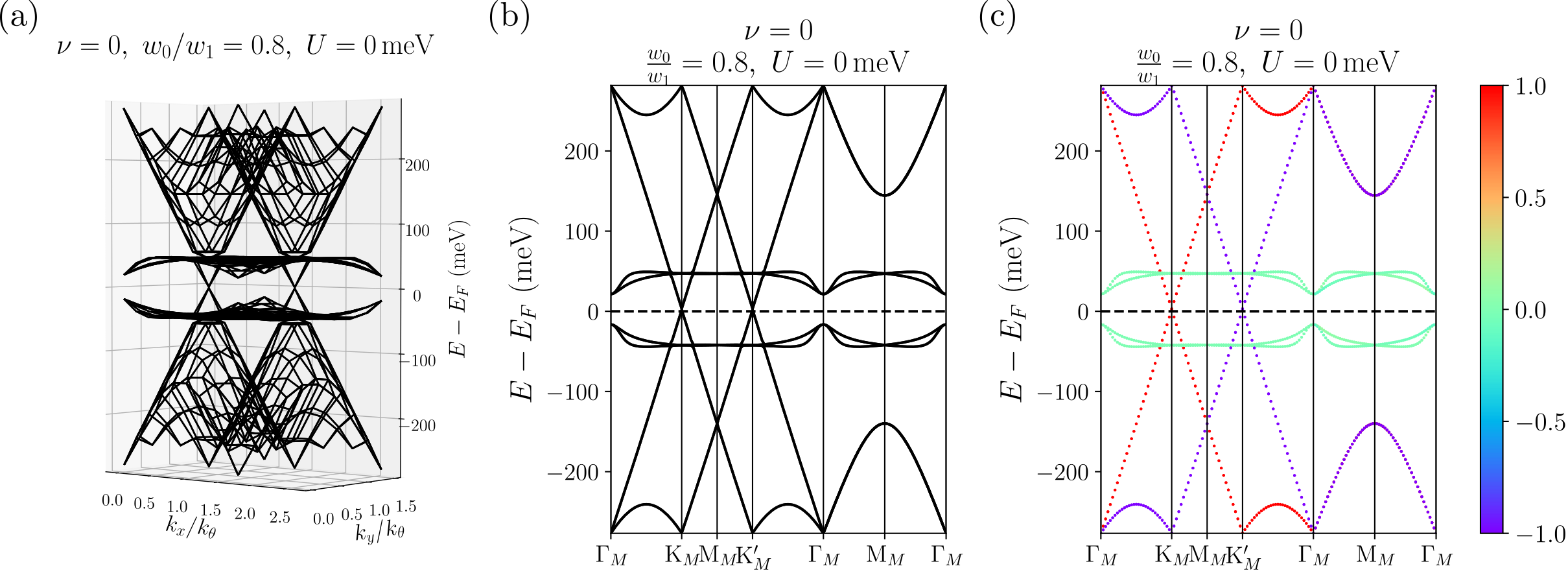
Several quantites can also be shown for each point in the band structure plots, for example, the valley polarization of each single body state. By diagonalizing the Hartree Fock Hamiltonian at a given along the high symmetry line, we can also obtain the corresponding wavefunction . For each given single body eigenstate of the Hartree Fock Hamiltonian, the valley polarization can be defined as follows:
| (S20) |
in which is the Pauli matrix acting in valley space. This quantity measures the valley polarization, therefore or if the state is valley polarized, and if there is a superposition between the two valleys. Fig. S5(c) shows the corresponding results of valley polarization for each state along the high symmetry line, using the same order parameter as Figs. S5(a) and S5(b). In this example, and using the color code visualization for , it can be seen clearly that the occupied flat bands are in intervalley coherent state at filling, as predicted in Refs. Bultinck et al. 2020b; Zhang et al. 2020; Lian et al. 2021.
Appendix C Additional Numerical Results
1 Numerical results at filling factor
In this appendix we provide additional HF results for various system sizes at filling factor . First in Fig. S6 we give the phase diagrams in the plane with a color code representing valley polarization on several momentum lattices: , and . Note that Fig. S6(c) was already provided in Fig. 1(a) and was added here for convenience. On the and momentum lattices, the HF calculation were performed at exact integer filling . For the momentum lattice (or any lattice of the size where is an integer), we removed four electrons from the exact integer filling, which is denoted by . Indeed, this lattice discretization exactly hits the Dirac points and , which induces degeneracy in the non-interacting band structure, plaguing the convergence of the HF self-consistent calculation. Removing four electrons improves the convergence by avoiding filling these degenerate states at Dirac points. As seen in these three phase diagrams, the positions of the three regions I, II and III do not strongly depend on the system size. We also notice that there is a small region with and around on momentum lattice located in region I, with small valley polarization, as opposed to the expected full polarization of region I. Such region does not show up in the other lattice discretizations. To test if this is a finite size effect or if this partially polarized region is induced by hitting exactly the and points, we also provide the plot of the dependence of several quantities for fixed on momentum lattice at filling with four electrons removed in Fig. S6(d) (note that a full phase diagram is computationally out of reach for this discretization). Similar to the momentum lattice, the momentum lattice also has and . However, the valley polarization shown in Fig. S6(d) does not drop around . This implies the region with small around on lattice is most probably due to size effects. We also provide the HF band structure obtained on lattice at filling factor in Fig. S7. Similar to the HF band structures in Fig. 2, we obtain one occupied valley polarized flat band in region I as shown in Fig. S7(a), a gapless metal state without valley polarization in region II shown in Fig. S7(b). We also obtained a state in region III shown in Fig. S7(c) on momentum lattice. When compared with Fig. 2(c) on momentum lattice in the main text, the result on lattice also have and , although the occupied TBG flat bands have different valley polarization.


To explain the regions I and III that are connected to the physics, we also provide the plots of and as a function of at zero displacement field for several momentum lattice sizes in Fig. S8. Similar to the calculation on lattice, we also removed four electrons from the integer filling on lattice. It can be clearly seen that the electrons are moving from Dirac bands into TBG flat bands, when gets larger. The transition point and the shape of these plots are not exactly the same, while they share very similar trends.
We now focus on the transition between regions III, I and II at fixed [see Fig. 1(a) in the main text]. The displacement field dependence of several physical quantities, including , , and , on different lattice sizes are shown in Fig. S9. In all these four diagrams, the system is in a valley and spin polarized state with one TBG flat band occupied when (which is in region I), and the valley polarization vanishes when (which is likely to be a metal state in region II). However, when the displacement is smaller than (which corresponds to region III), these four plots strongly change from one momentum lattice to another. Such a lattice size dependence could be related to the breakdown of the translation symmetry assumed for our HF order parameters (see Sec. III) as we have already argued in Sec. IV.
Finally, we address the question of translation symmetry breaking in region III. Using density matrix renormalization group, exact diagonalization, or HF, Refs. Kang and Vafek 2020; Soejima et al. 2020; Xie et al. 2021 found that a period- stripe phase in which translation symmetry is broken at momentum (see Fig. S1(b) and (c)) becomes energetically competitive in ordinary magic-angle TBG for and odd integer fillings. While a full-fledged HF calculation allowing for general translation symmetry breaking is beyond the scope of this article, we compute a phase diagram of the system at , by allowing symmetry breaking with the wave vector corresponding to the point. Denoting the moiré momentum at the point (see Fig. S1), we assume the HF order parameter of the system to be given by
| (S21) |
Compared to Eq. (S11), Eq. (S21) additionally allows for non-vanishing correlation between fermions whose momenta are separated by . To measure the degree of translation symmetry breaking, we define the quantity which is based on the norm of the off-diagonal (in momentum space) order parameter matrix elements
| (S22) |
ranges from zero, when there is no translation symmetry breaking, to a maximum value of (the factor 5 is due to 5 projected bands at in our calculation), when the fermions at and are fully coherent.
In Fig. S10, we provide the phase diagram of the system in the plane for an momentum lattice similar to Fig. 1 in the main text, allowing for translation symmetry breaking as defined in Eq. (S11). The translation symmetry breaking parameter vanishes in regions I and II, but indicates that the HF ground-state breaks the translation symmetry in region III. However, even in the presence of this translation symmetry breaking, the valley polarization shows qualitatively the same features in region III as in the case where the translation symmetry is enforced (see Fig. 1), namely electrons transfer from the Dirac valence bands into the TBG flat bands (as implied by ).
We note that there are other possible translation symmetry breaking momenta (e.g., Kekulé order) which have been discussed in TBG Xie et al. 2021; Kwan et al. 2021, and the charge transfers between Dirac and flat bands in TSTG may further allow the translation symmetry breaking momenta to shift to other values. Therefore, our results here allowing only translation breaking at may not give the ground state, and a future study allowing more translation breaking momenta is needed.

2 Numerical results at filling factor
In this appendix we present numerical results obtained on several momentum lattice sizes at integer filling . We start with the phase diagrams at integer filling . Figs. S11(a) and S12(a) show the intervalley coherence obtained on and momentum lattices. Other HF quantities on these system sizes at and are also shown in Figs. S11(b-c) and S12(b-c). Clearly the phase diagrams on the lattice are noisy, but the phase boundary where intervalley coherence vanishes is approximately the same as that of the larger sizes.


We also provide additional band structure plots in the metallic phase, namely the region III at . As shown in Fig. 3(b), the intervalley coherence can be a small but non-zero value in the metallic phase. We also observe that the intervalley coherence will decrease when becomes larger. This phenomenon can be observed in the HF band structures clearly. As shown in Fig. S13, the HF bands at and are intervalley coherent around points indicated by the valley polarization at each . Numerically, we observe that the intervalley coherence values are , and , respectively. The HF band structure also becomes more similar to the non-interacting band structure when becomes larger.

3 Numerical results at filling factor
Next, we provide some additional phase diagrams at filling on and lattices, which can be found in Figs. S14 and S15. Similar to other filling factors, the result obtained on smaller lattices, especially on is more noisy than the result on . However, the phase boundary where intervalley coherence disappears is not strongly affected.


4 Numerical results at filling factor
Similar to other fillings, we provide some phase diagrams obtained on and momentum lattices at filling factor . As shown in Figs. S16(a) and S17(a), these phase diagrams are similar to the results obtained on lattice, which has been discussed in the main text in Fig. 7(a). However, as shown in Fig. S16(b) and (c), the HF parameter value on lattice at filling is no longer zero, and the curves become noisy. The noisy curves can also be observed in the results obtained on momentum lattice at filling in Fig. S18 at and and at and . This observation means that there is a possible competing order with different Chern numbers in region II, as we mentioned in Sec.VII.
We also provide the Hartree-Fock band structure plots of two extra points in region III in Fig. S19. The discontinuous band structures at , and points can also be seen. Similar to Fig. 8(c), the HF bands at and points are gapless, showing that region III is a semimetallic state at filling.


Appendix D Understanding of the gaplessness of Dirac semimetal phases at all integer fillings at small
Our HF calculation shows that at each integer filling , there is a Dirac semimetal phase at small (region I of the phase diagram at each filling). Here we show that at even fillings , the gaplessness of the Dirac point in this Dirac semimetal phase is protected by a combined symmetry of the ground state given by combined with a valley rotation. At odd fillings , we show that the gapless Dirac point is protected by the symmetry within a invariant spin-valley flavor.
1 at all integer fillings
We first consider the case within region I of the phase diagram at each integer filling. At , the Dirac fermion sector and the TBG sector do not hop with each other, so the filling of electrons in each sector is conserved, which we denote as and , and the total filling is . Therefore, the ground state at a given filling is generically a tensor product of states within the two sectors:
| (S23) |
for certain .
We shall only discuss the case that the TSTG ground state has and at a given integer filling , and is given by the insulating ground state of TBG at filling (with no translation symmetry breaking) studied in Refs. Bultinck et al. 2020a; Lian et al. 2021. Under this assumption, the ground state at filling takes the form
| (S24) |
Our HF calculations showed that this is true (i.e., , , and the TBG sector is gapped) at for small enough in region I of all integer fillings. In particular, we have numerically checked that the HF Hamiltonian at has zero matrix elements hybridizing the Dirac fermions and TBG fermions, which confirms the direct product state nature of the ground state. Note that assumed here is required for the system to be strictly a Dirac semimetal with a point-like Fermi surface. At large , small electron and hole pockets may arise due to overlapping of the HF dispersions of the conduction and valence flat bands in the TBG sector, in which case the system is a metal (thus gapless) and will not be considered here.
We now show that the Dirac sector state is a gapless Dirac semimetal. We first recall that the interaction between the TBG sector and the Dirac sector is (see Eq. (25))
| (S25) |
where and stand for fermions in the Dirac and TBG sectors, respectively. As shown in Ref. Lian et al. 2021, in the flat-band limit at even fillings, or in the chiral-flat limit at any integer fillings , the insulating TBG ground state satisfies for some constants . Away from the flat-band limit or chiral-flat limit, we do not have the above exact relation, but in the HF approximation (which is the subject of study of this paper), provides a Hartree mean field with some constants for the Dirac fermions, provided that the translation symmetry is unbroken. Note that in the original sublattice basis is , where is the fermion basis in sublattices and ( stand for valley and spin), and is restricted within the first moiré BZ (since we project into the lowest 2 Dirac bands). Thus, the inter-sector interaction in Eq. (S25) solely yields a chemical potential to the Dirac fermion, which will not affect the Dirac sector ground state at fixed filling .
Therefore, the Dirac fermion ground state is solely determined by interactions within the Dirac fermion sector. Since the Dirac fermion sector alone is no different from the model of monolayer graphene, we expect the Dirac ground state to be a gapless Dirac semimetal, in analogy to that of the monolayer graphene. Here we give a heuristic understanding for the gaplessness of such a Dirac semimetal. Consider the Hartree-Fock approximation for Dirac fermions with a single-particle Hamiltonian and interaction . We now examine the possibility of an HF mean field order parameter of the form around . At the charge neutrality, the self-consistent HF equation then yields (for fixed spin and valley )
| (S26) |
Assume the maximal value of among all is , and we take the interaction in Eq. (14), we have
| (S27) |
where is the UV momentum cutoff. Note that the above bound is quite lose, with all in the integral relaxed to , while in fact decays at least as at large according to Eq. (S27) above. Nevertheless, this yields a loose bounding condition
| (S28) |
where . In this paper we have nm, meV, and meVnm. For monolayer graphene, nm-1 (nm is the graphene lattice constant), which yields . In our practical calculation, we only keep the lowest two Dirac bands, which corresponds to nm-1, and yields . In either case, , and we find the HF mass is bounded to . So the Dirac ground state is gapless.
Therefore, we find the TSTG ground state is a gapless Dirac semimetal at and .
2 at even integer fillings
In this case, the interlayer potential yields a hopping term between the Dirac fermion sector and the TBG sector as given in Eq. (21).
The TBG ground state at even fillings or is a gapped intervalley coherent state given by the wavefunction Bultinck et al. 2020a; Lian et al. 2021
| (S29) |
where is the TBG Chern band basis defined in Eq. (20), is the intervalley coherent spontaneous symmetry breaking phase, and , are the set for the spin index summation. Noting that (under our gauge fixing), we see the TBG ground state has a remaining antiunitary symmetry combined with valley rotation:
| (S30) |
where is the valley rotation generator. Moreover, note that the absence of a mass term in the Dirac ground state in 1 indicates that the Dirac ground state also obeys the antiunitary symmetry in Eq. (S30). So the even filling TSTG ground state at (Eq. (S24)), which is a Dirac semimetal tensor producted with an intervalley coherent TBG ground state, respects the symmetry.
When , since in Eq. (21) only contains intravalley hoppings and respect the symmetry, we know that also respects the antiunitary symmetry in Eq. (S30). Therefore, provided is small enough, we expect the symmetry to remain respected by the TSTG ground state. The symmetry then protects the gaplessness of Dirac points, similar to the protection by symmetry (see for example Ref. Song et al. 2021). This is in agreement with our findings in for region I of the TSTG phase diagram, where the ground state is an intervalley coherent Dirac semimetal.
3 at odd integer fillings
At odd integer fillings , the TBG ground state is shown in Ref. Lian et al. 2021 to be a Chern insulator of Chern number , which breaks the symmetry. However, the TBG ground state in this case always has at least one valley-spin flavor fully empty (which is exact, since the number of electrons in each spin-valley flavor () in TBG or TSTG is conserved). More concretely, the TBG ground state is valley polarized and has one band in flavor () occupied and all the other bands empty; the TBG ground state occupies 2 intervalley coherent bands in the spin sector, and one band in flavor (). In both cases, the valley-spin flavor () is fully empty. Therefore, the symmetry is preserved within the valley-spin flavor () of TBG.
On the other hand, at , the Dirac ground state of the TSTG also preserves the symmetry because of the absence of a Dirac mass. Therefore, we conclude that the TSTG ground state in region I of the odd fillings at preserves the symmetry in the sector of valley-spin flavor ().
When , in Eq. (21) respects the symmetry and only contains hoppings within each spin-valley flavor. Therefore, for small enough , we expect the symmetry within the valley-spin flavor () to remain respected by the odd-filling TSTG ground state. The symmetry therefore at least protects the gapless Dirac nodes in the empty valley-spin flavor (), ensuring the TSTG ground state in region I of odd fillings at to be a gapless Dirac semimetal.