跳到论文正文
W Papers独立论文阅读器 arXiv:2106.14818 论文正文 计算阅读时间 · 0%
引用这篇论文根据当前论文元数据生成,正式投稿前建议核对。


License: arXiv.org perpetual non-exclusive license
arXiv:2106.14818v2 [math.CA] 17 Dec 2021

New bounds on Cantor maximal operatorsThanks: PS was supported by project PICT 2015-3675 (ANPCyT) and by an NSERC discovery grant. VS was in part supported by the Academy of Finland. We also acknowledge support from the Institut Mittag-Leffler via the “Fractal Geometry and Dynamics” research program, where this project started.

Pablo Shmerkin Email address: pshmerkin@math.ubc.ca Address: Department of Mathematics, the University of British Columbia, 1984 Mathematics Road Vancouver, BC, V6T 1Z2, Canada and Ville Suomala Email address: ville.suomala@oulu.fi Address: Research Unit of Mathematical Sciences, P.O.Box 8000, FI-90014, University of Oulu, Finland
Abstract.

We prove LpL^{p} bounds for the maximal operators associated to an Ahlfors-regular variant of fractal percolation. Our bounds improve upon those obtained by I. Łaba and M. Pramanik and in some cases are sharp up to the endpoint. A consequence of our main result is that there exist Ahlfors-regular Salem Cantor sets of any dimension >1/2>1/2 such that the associated maximal operator is bounded on L2​(ℝ)L^{2}(\mathbb{R}). We follow the overall scheme of Łaba-Pramanik for the analytic part of the argument, while the probabilistic part is instead inspired by our earlier work on intersection properties of random measures.

2020 Mathematics Subject Classification
Primary: 42B25; Secondary: 28A80, 60G57.

1. Introduction

1.1. Maximal functions associated to singular measures

One of the most classical results in real analysis is the LpL^{p} boundedness of the Hardy-Littlewood maximal operator, which can be restated as follows: let ν\nu be Lebesgue measure on the unit ball of ℝd\mathbb{R}^{d}. Then the maximal operator

M¯ν​f​(x)=supr>0∫|f⁡(x+r​y)|​𝑑ν​(y)\overline{M}_{\nu}f(x)=\sup_{r>0}\int|f(x+ry)|\,d\nu(y)

is bounded on LpL^{p} for p>1p>1. It makes sense to study such operators M¯ν\overline{M}_{\nu} also when ν\nu is replaced by other, singular measures; one would expect its boundedness properties to reflect in some sense the geometry of the measure ν\nu. The case in which ν\nu is surface area on the (d−1)(d-1)-dimensional sphere is the celebrated spherical maximal theorem of Stein [10], for the case d≥3d\geq 3, and Bourgain [1], in the more challenging case d=2d=2: in this case M¯ν\overline{M}_{\nu} is bounded on LpL^{p} if and only if p>d/(d−1)p>d/(d-1). A large body of related work exists in which ν\nu is replaced by Hausdorff measure on more general manifolds under curvature assumptions, or is assumed to satisfy a power Fourier decay bound; see for example [7].

Neither of the classical approaches gives information if ν\nu is a singular measure on the real line, since the concept of submanifold or curvature is not available and the required Fourier decay cannot possibly hold. Nevertheless, it is natural to study this problem when ν\nu is, for example, Hausdorff measure on a Cantor set of dimension <1<1. A first breakthrough in this direction was achieved by Łaba and Pramanik in [6]. In order to state their result, we introduce the restricted (or single-scale) version of the maximal operator, defined as

Mν​f​(x)=supr∈[1,2]∫|f⁡(x+r​y)|​𝑑ν​(y).M_{\nu}f(x)=\sup_{r\in[1,2]}\int|f(x+ry)|\,d\nu(y).

The restricted version is easier to handle technically and, in any case, its mapping properties can be used in some cases to derive bounds also for certain unrestricted operators - see §1.3 below.

Theorem 1.1 ([6, Theorem 1.3]).

For any s∈(2/3,1)s\in(2/3,1) there exists a measure ν\nu supported on a Cantor set of Hausdorff dimension ss, such that the associated restricted maximal operator Mν​f​(x)M_{\nu}f(x) is bounded from Lp​(ℝ)L^{p}(\mathbb{R}) to Lq​(ℝ)L^{q}(\mathbb{R}) for p>(2−s)/sp>(2-s)/s and q∈[p,p​s/(2−2​s)]q\in[p,ps/(2-2s)].

The Cantor set and the measure ν\nu arising in the proof of Theorem 1.1 are obtained through an ad-hoc random iterative process; no almost sure statements with respect to an underlying distribution on Cantor measures are made.

In subsequent work, Łaba [5] considered maximal operators for certain self-similar Cantor sets in which the randomization only occurs in the first level pattern of the construction. While stopping short of proving LpL^{p} estimates in this case, her results cover Cantor sets of arbitrarily small dimension, in addition to providing the first results in the area for self-similar examples.

In order to discuss the sharpness of Theorem 1.1, let us note the following simple lemma.

Lemma 1.2.

If ν\nu is a finite measure giving positive mass to a set of Hausdorff dimension <t<t, then MνM_{\nu} cannot be bounded from L1/t​(ℝ)L^{1/t}(\mathbb{R}) to Lq​(ℝ)L^{q}(\mathbb{R}) for any q∈[1,+∞]q\in[1,+\infty].

Proof.

If ν⁡(A)>0\nu(A)>0 for a set AA of Hausdorff dimension <t<t, then by the mass distribution principle (see e.g. [2, Proposition 4.9]) there are s<ts<t and a point x0≠0x_{0}\neq 0 in the support of ν\nu such that for a sequence δi↓0\delta_{i}\downarrow 0, we have

ν⁡([x0−δi,x0+δi])>δis.\nu([x_{0}-\delta_{i},x_{0}+\delta_{i}])>\delta_{i}^{s}.

Let fif_{i} be the indicator of the interval [x0−2​δi,x0+2​δi][x_{0}-2\delta_{i},x_{0}+2\delta_{i}]. If x∈[−x0,0]x\in[-x_{0},0] then taking r=1−x/x0r=1-x/x_{0} in the definition of MνM_{\nu} we see that Mν​fi​(x)>δisM_{\nu}f_{i}(x)>\delta_{i}^{s}, and hence ‖Mν​fi‖Lq​(ℝ)>x01/q​δis\|M_{\nu}f_{i}\|_{L^{q}(\mathbb{R})}>x_{0}^{1/q}\delta_{i}^{s}. On the other hand, ‖fi‖Lp​(ℝ)≤(4​δi)1/p\|f_{i}\|_{L^{p}(\mathbb{R})}\leq(4\delta_{i})^{1/p}. Taking δi↓0\delta_{i}\downarrow 0, we see that MνM_{\nu} cannot be bounded from Lp​(ℝ)L^{p}(\mathbb{R}) to Lq​(ℝ)L^{q}(\mathbb{R}) if p≤1/tp\leq 1/t. ∎

Note that for all dimension values s∈(2/3,1)s\in(2/3,1), there is a gap between the admissible values p>(2−s)/sp>(2-s)/s provided by Theorem 1.1 and the barrier p≥1/sp\geq 1/s arising from Lemma 1.2. It is natural to ask what is the optimal range of pp, given ss, see [6, Remark 3 on p. 350].

In this article we obtain a version of the theorem of Łaba and Pramanik with improved exponents and dimension bounds, which in some cases close the gap indicated above. In particular, we show that there are measures supported on Ahlfors-regular Salem Cantor sets of any dimension >1/2>1/2 satisfying non-trivial maximal operator bounds (while we recall that in [6] the Cantor sets must have dimension >2/3>2/3). Our constructions are still random at all scales, but fall into a widely studied class of random measures and sets closely related to the well known fractal percolation model. The method can be easily extended to other random models. Moreover, we are able to simplify various aspects of the rather involved original proof of Theorem 1.1. Before stating our main result, Theorem 1.3, we introduce the random model it involves.

1.2. Ahlfors regular random sets and measures

Let 𝒟n\mathcal{D}_{n} denote the level nn dyadic intervals of ℝ\mathbb{R}:

𝒟n={[k​2−n,(k+1)​2−n]:k∈ℤ}.\mathcal{D}_{n}=\{[k2^{-n},(k+1)2^{-n}]\,:\,k\in\mathbb{Z}\}\,.

Let 0<s<10<s<1 and let an∈{1,2}a_{n}\in\{1,2\} such that

2s​n−1<βn≤2s​n​ for all ​n∈ℕ,where ​βn=∏i=1nan.2^{sn-1}<\beta_{n}\leq 2^{sn}\text{ for all }n\in\mathbb{N},\quad\text{where }\beta_{n}=\prod_{i=1}^{n}a_{n}.

Starting with the interval A0=[1,2]A_{0}=[1,2], we inductively construct random sets AnA_{n} as follows. If an=2a_{n}=2, set An+1=AnA_{n+1}=A_{n}. Otherwise, if an=1a_{n}=1, choose, for each I∈𝒟nI\in\mathcal{D}_{n} such that I⊂AnI\subset A_{n}, one of the 22 dyadic sub-intervals of II, with all choices being uniform and independent of each other and the previous steps. Let An+1A_{n+1} be the union of the chosen I∈𝒟nI\in\mathcal{D}_{n}. Then {An}\{A_{n}\} is a decreasing sequence of nonempty sets (each AnA_{n} consists of βn\beta_{n} pairwise disjoint dyadic intervals of length 2−n2^{-n}), and we set

A=⋂n=1∞An.A=\bigcap_{n=1}^{\infty}A_{n}\,.

Let us further define

νn=2nβn​𝟏​[An],\nu_{n}=\frac{2^{n}}{\beta_{n}}\mathbf{1}[A_{n}], (1.1)

and note that

νn≤2⋅2n⁡(1−s)\nu_{n}\leq 2\cdot 2^{n(1-s)} (1.2)

and that νn\nu_{n} is zero off a set of Lebesgue measure at most 2n⁡(1−s)2^{n(1-s)}.

It is easy to check (see e.g. [2, Proposition 1.7]) that νn\nu_{n} converges in the weak∗-sense to a Borel probability measure ν\nu and that spt⁡ν=A\spt\nu=A. Moreover, ν\nu is Ahlfors ss-regular, that is, there exists a (deterministic) constant C>0C>0 such that

C−1⋅rs≤ν⁡(B⁡(x,r))≤C⋅rsC^{-1}\cdot r^{s}\leq\nu(B(x,r))\leq C\cdot r^{s}

for all x∈Ax\in A and all r∈(0,1]r\in(0,1]. In particular, the Hausdorff dimension of AA, and of ν\nu, equal ss (deterministically) and

ν​(I),νn​(I)\displaystyle\nu(I),\nu_{n}(I) ≤3​|I|s​ for all intervals ​I⊂[0,1],\displaystyle\leq 3|I|^{s}\text{ for all intervals }I\subset[0,1]\,, (1.3)

where |I||I| denotes the length of the interval. Note that in the above notation, and also in what follows, we will often identify the functions νn\nu_{n} with the measure d​νn​(x)=νn​d​xd\nu_{n}(x)=\nu_{n}dx. This also applies to Cartesian powers of νn\nu_{n}.

1.3. Main result

We can now state our main result:

Theorem 1.3.

Let s∈(1/2,1)s\in(1/2,1) and let d=2​⌈12−2​s−1⌉d=2\lceil\tfrac{1}{2-2s}-1\rceil. Further, define

θ0\displaystyle\theta_{0} =d​s+1−d2>0,\displaystyle=\frac{ds+1-d}{2}>0,
ξ0\displaystyle\xi_{0} =d+1−(d+2)​s≥0\displaystyle=d+1-(d+2)s\geq 0

If ν\nu is the random measure defined above, then almost surely MνM_{\nu} is bounded from Lp​(ℝ)L^{p}(\mathbb{R}) to Lq​(ℝ)L^{q}(\mathbb{R}) for all

p>p0:=(2+d)​θ0+d​ξ0(1+d)​θ0+(d−1)​ξ0p>p_{0}:=\frac{(2+d)\theta_{0}+d\xi_{0}}{(1+d)\theta_{0}+(d-1)\xi_{0}}

and

p≤q≤pp0−1.p\leq q\leq\frac{p}{p_{0}-1}.

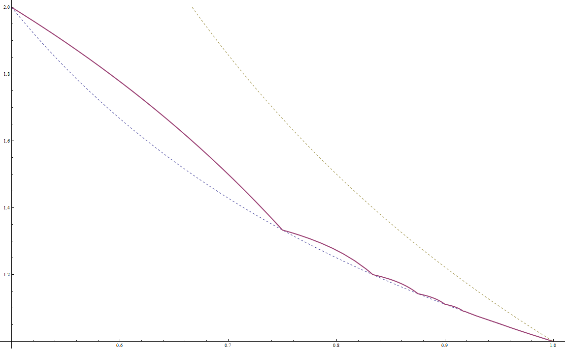
See Figure 1 for an illustration. We make some remarks on the statement of theorem and its proof.
Refer to caption
Figure 1. The solid curve shows the value of p0=p0​(s)p_{0}=p_{0}(s) provided by Theorem 1.3 for each s∈(1/2,1)s\in(1/2,1), so that MνM_{\nu} is a.s. bounded on LpL^{p} for p>p0p>p_{0}. The lower dashed curve is 1/s1/s; by Lemma 1.2, the maximal operator can’t be bounded on LpL^{p} for p<1/sp<1/s. The upper dashed curve is the value p0=(2−s)/sp_{0}=(2-s)/s, s>2/3s>2/3, given by the theorem of Łaba-Pramanik (Theorem 1.1)
Remark 1.4.

As remarked in Lemma 1.2, MνM_{\nu} is not bounded from LpL^{p} to any LqL^{q} if p<1/sp<1/s. In the special case s=1−12​d′s=1-\frac{1}{2d^{\prime}}, d′≥2d^{\prime}\geq 2, the above theorem shows that MνM_{\nu} is bounded on LpL^{p} for any p>1/sp>1/s. So Theorem 1.3 provides the first instance of a sharp bound for maximal operators associated to Cantor sets of fractional dimension (up to the endpoint). The lower bound p0p_{0} provided by Theorem 1.3 is continuous in ss, so the theorem also provides nearly sharp bounds for ss close to 1−12​d′1-\frac{1}{2d^{\prime}} for d′≥2d^{\prime}\geq 2, and also for ss slightly larger than 1/21/2 (but it provides no information for s≤1/2s\leq 1/2).

Remark 1.5.

Unlike the construction of [6], the measure ν\nu is Ahlfors-regular. This may be seen as a desirable geometrical property that holds in all classical examples such as smooth manifolds. Additionally, as a direct consequence of [8, Theorem 14.1], the measure ν\nu is almost surely a Salem measure - again as is the case for manifolds for non-zero Gaussian curvature.

Remark 1.6.

While we have chosen the model described in Section 1.2 for concreteness, the argument of the proof extends to a wide class of subdivision fractals - see [8, §5.2].

Remark 1.7.

For proving Theorem 1.3, we follow [6] (with some minor simplifications) to reduce the claim to a purely geometric fact regarding intersections of random sets with lines, see Theorem 2.2 below. Our proof differs from that of [6] in the probabilistic argument to establish the intersection result; it is here that our argument is more effective, and perhaps also simpler. It is inspired by our earlier work [8, 9]. A new aspect is that we also need to consider intersections with lines which are not “transversal” and this requires a more delicate analysis.

We mention some direct applications of Theorem 1.3. For the first two we follow [6]. We fix s∈(1/2,1)s\in(1/2,1) and the threshold p0p_{0} provided by the theorem.

  1. (1)

    Theorem 1.3 implies the boundedness of the unrestricted maximal operator

    M¯ν​f​(x)=supr>0∫f⁡(x+r​y)​𝑑ν​(y)\overline{M}_{\nu}f(x)=\sup_{r>0}\int f(x+ry)\,d\nu(y)

    for p=q>p0p=q>p_{0}, by the argument in [6, Section 7] which is very general and does not rely on the specific random construction in that paper. For q>pq>p a similar result holds but one needs to weigh the unrestricted operator for scaling reasons, see [6, Eq. (1.4)].

  2. (2)

    Maximal operator bounds imply differentiation results. In particular, in the context of Theorem 1.3, if f∈Lp​(ℝ)f\in L^{p}(\mathbb{R}) with p>p0p>p_{0}, then

    f⁡(x)=limr→0∫f⁡(x+r​y)​𝑑ν​(y)f(x)=\lim_{r\to 0}\int f(x+ry)\,d\nu(y)

    for a.e. x∈ℝx\in\mathbb{R}. See [6, §8.1].

  3. (3)

    Finally, maximal operator bounds also yield information about the Lebesgue measure of the union of families of Cantor sets. Namely, if the Borel set E⊂ℝE\subset\mathbb{R} contains a set of the form x+r​Ax+rA (for some rr depending on xx) for each xx in a set FF of positive Lebesgue measure, then EE has positive Lebesgue measure. Indeed, Mν​𝟏E​(x)=1M_{\nu}\mathbf{1}_{E}(x)=1 for all x∈Fx\in F, which immediately yields |E|>0|E|>0 (for this it is enough to have a bound ‖Mν​f‖q≤C​‖f‖p\|M_{\nu}f\|_{q}\leq C\|f\|_{p} for any p<∞p<\infty). Similar problems for other classes of Cantor sets have been considered in [3, 5]; the Cantor sets in those papers are (essentially) deterministic and the conclusions are therefore much weaker.

2. Reduction of the main theorem to intersection estimates

2.1. From intersection estimates to maximal operator bounds

We will derive our main theorem by analyzing the intersections of the self-products of ν\nu with lines. To reduce the main theorem to such intersection estimates, we will use the following theorem that can be inferred from the framework of [6].

Theorem 2.1.

For n∈ℕn\in\mathbb{N}, let An⊂[1,2]A_{n}\subset[1,2] be a finite union of closed intervals such that An+1⊂AnA_{n+1}\subset A_{n}. Denote νn=|An|−1​𝟏​[An]\nu_{n}=|A_{n}|^{-1}\mathbf{1}[A_{n}] and σn=νn+1−νn\sigma_{n}=\nu_{n+1}-\nu_{n}. Suppose that νn\nu_{n} converges in the weak*-sense to a measure ν\nu. Furthermore assume that d≥2d\geq 2 is an even integer and there are constants θ,ξ,K>0\theta,\xi,K>0, such that for all measurable choices of r:[−4,0]→[1,2]r\colon[-4,0]\to[1,2] and for all Ω⊂[0,1]\Omega\subset[0,1] it holds that

|Ω|1−d​∫Ωd∫∏j=1dσk​(z−xjr⁡(xj))​𝑑z​𝑑x\displaystyle|\Omega|^{1-d}\int_{\Omega^{d}}\int\prod_{j=1}^{d}\sigma_{k}\left(\frac{z-x_{j}}{r(x_{j})}\right)\,dz\,dx ≤K​exp⁡(−θ​k),\displaystyle\leq K\exp(-\theta k)\,, (2.1)
|Ω|−1−d​∫Ωd+2∫∏j=1d+2σk​(z−xjr⁡(xj))​𝑑z​𝑑x\displaystyle|\Omega|^{-1-d}\int_{\Omega^{d+2}}\int\prod_{j=1}^{d+2}\sigma_{k}\left(\frac{z-x_{j}}{r(x_{j})}\right)\,dz\,dx ≤K​exp⁡(ξ​k).\displaystyle\leq K\exp(\xi k)\,. (2.2)

Then MνM_{\nu} is bounded from Lp​(ℝ)L^{p}(\mathbb{R}) to Lq​(ℝ)L^{q}(\mathbb{R}), whenever

p>p0:=(2+d)​θ+d​ξ(1+d)​θ+(d−1)​ξp>p_{0}:=\frac{(2+d)\theta+d\xi}{(1+d)\theta+(d-1)\xi}

and

p≤q≤pp0−1.p\leq q\leq\frac{p}{p_{0}-1}.

Since this is not stated in this form in [6], in the rest of this section we discuss the main steps of the proof, referring to [6] for most details. We point out two differences between our approach and that of Łaba and Pramanik that are not essential but help us simplify parts of the argument. The first is that we don’t have an explicit split between “internal” and “transverse” intersections. These concepts from [6] were inspired by Bourgain’s proof of the boundedness of the circular maximal operator, but such a dichotomy is not needed in our approach. The second is that they discretize the family of measurable functions rr at each scale at the “deterministic” stage, while we perform a similar discretization in the probabilistic part of the argument.

Roughly speaking, Theorem 2.1 follows a classical scheme involving discretization, linearization, dualization and interpolation arguments, although extra care is required at some steps. Since ν\nu is fixed, we denote M=MνM=M_{\nu} for simplicity. Firstly, using that q≥pq\geq p it is enough to show that MM is bounded from Lp​[0,1]L^{p}[0,1] to Lq​(ℝ)L^{q}(\mathbb{R}); this is due to the fact that we are dealing with the restricted operator (r∈[1,2]r\in[1,2]); see the proof of [6, Lemma 3.1] for details. Next, for f∈C⁡[0,1]f\in C[0,1] define

Mk​f​(x)=supr∈[1,2]|f⁡(x+r​y)​σk​(y)​d​y|.M_{k}f(x)=\sup_{r\in[1,2]}\left|f(x+ry)\sigma_{k}(y)\,dy\right|.

It is an easy consequence of the weak∗-convergence of νn\nu_{n} to ν\nu that

M​f≤N​f+∑k=1∞Mk​|f|,where ​N​f​(x)=supr∈[1,2]∫|f⁡(x+r​y)|​d​ν1​(y).Mf\leq Nf+\sum_{k=1}^{\infty}M_{k}|f|,\quad\text{where }Nf(x)=\sup_{r\in[1,2]}\int|f(x+ry)|d\nu_{1}(y).

As ν1\nu_{1} is dominated by a bounded multiple of Lebesgue measure, this reduces the problem to the study of the operators MkM_{k}.

Next, we linearize the problem. It is easy to see that for f∈C⁡[0,1]f\in C[0,1],

∥Mkf(x)∥Lq​(ℝ)≤4supr:[−4,0]→[1,2]​ measurable∥Mr,kf(x)∥Lq​(ℝ),\|M_{k}f(x)\|_{L^{q}(\mathbb{R})}\leq 4\sup_{r\colon[-4,0]\to[1,2]\text{ measurable}}\|M_{r,k}f(x)\|_{L^{q}(\mathbb{R})},

where Mk,rM_{k,r} is the (linear) operator

Mk,r​f​(x)=∫f⁡(z)​σk​(z−xr⁡(x))​𝑑z.M_{k,r}f(x)=\int f(z)\sigma_{k}\left(\frac{z-x}{r(x)}\right)\,dz.

See [6, Proposition 3.2] for details. (It is enough to consider x∈[−4,0]x\in[-4,0] since r⁡(x)∈[1,2]r(x)\in[1,2] and σk\sigma_{k} is supported on [1,2][1,2].) Thus the claim will follow if

‖Mk,r‖Lp​[0,1]→Lq​[−4,0]≤δk\|M_{k,r}\|_{L^{p}[0,1]\to L^{q}[-4,0]}\leq\delta_{k} (2.3)

for some summable sequence (δk)(\delta_{k}) independent of the choice of rr. The adjoint operator to Mk,rM_{k,r} is

Mk,r∗​g​(z)=∫g⁡(x)​σk​(z−xr⁡(x))​𝑑x.M^{*}_{k,r}g(z)=\int g(x)\sigma_{k}\left(\frac{z-x}{r(x)}\right)\,dx.

Using interpolation and duality, one can see that if q0≥2q_{0}\geq 2 and the restricted bound

‖Mk,r∗​𝟏​[Ω]‖Lq0​[−4,0]≤C​2−ζ​k​|Ω|q0−1q0\|M^{*}_{k,r}\mathbf{1}[\Omega]\|_{L^{q_{0}}[-4,0]}\leq C2^{-\zeta k}|\Omega|^{\tfrac{q_{0}-1}{q_{0}}} (2.4)

holds for all Ω⊂[0,1]\Omega\subset[0,1] and some constants C,ζ>0C,\zeta>0, then (2.3) holds for

p>q0q0−1,q=(q0−1)​p,p>\frac{q_{0}}{q_{0}-1},\quad q=(q_{0}-1)p\,,

for an exponentially decaying sequence (δk)(\delta_{k}) (depending on p,qp,q). Then it also holds for q∈[p,(q0−1)​p]q\in[p,(q_{0}-1)p]. See [6, Lemma 3.4] for the details of this step, that requires special care. (This is where we use the hypothesis on qq.)

On the other hand, it is easy to check (see [6, Proof of Prop. 4.2]) that if d≥2d\geq 2 is an even integer, then

‖Mk,r∗​𝟏​[Ω]‖Ld​[−4,0]d=∫Ωd∫∏j=1dσk​(z−xjr⁡(xj))​𝑑z​𝑑x.\|M^{*}_{k,r}\mathbf{1}[\Omega]\|_{L^{d}[-4,0]}^{d}=\int_{\Omega^{d}}\int\prod_{j=1}^{d}\sigma_{k}\left(\frac{z-x_{j}}{r(x_{j})}\right)\,dz\,dx. (2.5)

Let u∈(0,1]u\in(0,1] satisfy u>d​ξ(d+2)​θ+d​ξu>\tfrac{d\xi}{(d+2)\theta+d\xi} (where θ,ξ\theta,\xi are as in Theorem 2.1). Let qu∈(d,d+2]q_{u}\in(d,d+2] satisfy

1qu=ud+1−ud+2\frac{1}{q_{u}}=\frac{u}{d}+\frac{1-u}{d+2}

so that qu=d⁡(d+2)2​u+dq_{u}=\tfrac{d(d+2)}{2u+d} (and ququ−1=d⁡(d+2)d⁡(d+1)−2​u\tfrac{q_{u}}{q_{u}-1}=\tfrac{d(d+2)}{d(d+1)-2u}). Using Hölder’s inequality,

‖Mk,r∗​𝟏​[Ω]‖qu≤‖Mk,r∗​𝟏​[Ω]‖du​‖Mk,r∗​𝟏​[Ω]‖d+21−u.\displaystyle\|M^{*}_{k,r}\mathbf{1}[\Omega]\|_{q_{u}}\leq\|M^{*}_{k,r}\mathbf{1}[\Omega]\|_{d}^{u}\,\|M^{*}_{k,r}\mathbf{1}[\Omega]\|_{d+2}^{1-u}.

Recalling the assumptions (2.1)–(2.2), we arrive at

‖Mk,r∗​𝟏​[Ω]‖qu\displaystyle\|M^{*}_{k,r}\mathbf{1}[\Omega]\|_{q_{u}} ≤K′​|Ω|u⁡(d−1)d+(1−u)​(d+1)(d+2)​exp⁡(k⁡(−u​θd+(1−u)​ξd+2))\displaystyle\leq K^{\prime}|\Omega|^{\tfrac{u(d-1)}{d}+\tfrac{(1-u)(d+1)}{(d+2)}}\exp\left(k\left(\frac{-u\theta}{d}+\frac{(1-u)\xi}{d+2}\right)\right)
=K′​|Ω|qu−1qu​exp⁡(−ζ​k),\displaystyle=K^{\prime}|\Omega|^{\tfrac{q_{u}-1}{q_{u}}}\exp(-\zeta k)\,,

for some ζ>0\zeta>0 provided u>d​ξ(d+2)​θ+d​ξu>\tfrac{d\xi}{(d+2)\theta+d\xi}.

After some algebra, letting u↓d​ξ(d+2)​θ+ξu\downarrow\tfrac{d\xi}{(d+2)\theta+\xi} completes the proof of Theorem 2.1.

2.2. Reduction of the main result to probabilistic intersection estimates

Let us continue to denote

σn=νn+1−νn,\sigma_{n}=\nu_{n+1}-\nu_{n}, (2.6)

where νn\nu_{n} is as in (1.1).

Using Theorem 2.1, the following probabilistic estimate will easily imply our main result, Theorem 1.3.

Theorem 2.2.

Let σk\sigma_{k} be as in (2.6) and fix d≥2d\geq 2. Let

Φk(d)=supr:[−4,0]→[1,2],Ω⊂[0,1]|Ω|1−d∫Ωd∫∏j=1dσk(z−xjr⁡(xj))dzdx,\Phi_{k}^{(d)}=\sup_{r\colon[-4,0]\to[1,2],\Omega\subset[0,1]}|\Omega|^{1-d}\int_{\Omega^{d}}\int\prod_{j=1}^{d}\sigma_{k}\left(\frac{z-x_{j}}{r(x_{j})}\right)\,dz\,dx, (2.7)

where the supremum runs over all measurable functions rr. Note that Φk(d)\Phi_{k}^{(d)} is a random variable.

Then for all k∈ℕk\in\mathbb{N}:

  1. (1)

    If s>1−1ds>1-\tfrac{1}{d} and 0<θ<(d​s+1−d)/20<\theta<(ds+1-d)/2, then Φk(d)≤K​exp⁡(−θ​k)\Phi_{k}^{(d)}\leq K\exp(-\theta k),

  2. (2)

    If s≤1−1ds\leq 1-\tfrac{1}{d} and ξ>d−1−d​s≥0\xi>d-1-ds\geq 0 , then Φk(d)≤K​exp⁡(ξ​k)\Phi_{k}^{(d)}\leq K\exp(\xi k),

where KK is an almost surely finite random variable (depending on d,s,θ,ξd,s,\theta,\xi).

We will prove Theorem 2.2 in Section 3. Theorem 1.3 is a simple consequence of Theorems 2.1 and 2.2. Indeed, given s>1/2s>1/2, then d=2​⌈12−2​s−1⌉d=2\lceil\tfrac{1}{2-2s}-1\rceil satisfies 1−1d<s≤1−1d+21-\tfrac{1}{d}<s\leq 1-\tfrac{1}{d+2}. Theorem 2.2 ensures that if 0<θ<(d​s+1−d)/20<\theta<(ds+1-d)/2 and ξ>d+1−(d+2)​s\xi>d+1-(d+2)s, then the hypotheses of Theorem 2.1 are satisfied. Theorem 1.3 follows by letting θ↑θ0=(d​s+1−d)/2\theta\uparrow\theta_{0}=(ds+1-d)/2 and ξ↓ξ0=d+1−(d+2)​s\xi\downarrow\xi_{0}=d+1-(d+2)s.

Remark 2.3.

Theorem 2.2 holds for all integers d≥2d\geq 2, but when we apply it to prove Theorem 1.3, we restrict to even values of dd to be able to use Theorem 2.1. The assumption that dd is even is essential in the proof of Theorem 2.1, since (2.5) fails for dd odd.

3. Proof of Theorem 2.2

3.1. Outline of proof

In this section we prove Theorem 2.2 which, as explained above, implies Theorem 1.3. We start by giving an outline of the proof. It is easy to recast the inner integral in the definition of Φk(d)\Phi_{k}^{(d)} given in (2.7) as an integral of the dd-fold cartesian product λn:=σn×⋯×σn\lambda_{n}:=\sigma_{n}\times\cdots\times\sigma_{n} over a line Lx,rL_{x,r} determined by the xjx_{j} and the choice of the function rr. Because the functions σk\sigma_{k} are highly singular, the inner integral blows up on the diagonals xi=xjx_{i}=x_{j}. On the other hand, if the xix_{i} are well separated (essentially what is called a “transverse intersection” in [6]) one would expect a large amount of cancellation. Indeed, a stochastic induction in nn coupled with Hoeffding-type estimates can be used to show that, for the fixed line Lx,rL_{x,r} the random variable

Xn​(x,r)=∫Lx,rλn​d​ℋ1.X_{n}(x,r)=\int_{L_{x,r}}\lambda_{n}\,d\mathcal{H}^{1}.

decays exponentially in nn, with overwhelming probability. Here the line Lx,rL_{x,r} is fixed, but because the probability that Xn​(x,r)X_{n}(x,r) does not decay exponentially is so small (sub-exponential), it follows tht Xn​(xj,rj)X_{n}(x_{j},r_{j}) decay exponentially, with a uniform bound, for any collection Lxj,rjL_{x_{j},r_{j}} of transversal lines of size exponential in nn. By choosing the (xj,rj)(x_{j},r_{j}) densely in the parameter space, a deterministic continuity bound in xx and rr can then be used to extend the estimate to all transversal lines. So far, this scheme is similar to that of [9]. However, we need to deal also with non-transversal lines, that is lines for which |xi−xj||x_{i}-x_{j}| is small for some i≠ji\neq j (roughly the “internal tangencies” of [6]). For such lines Xn​(x,r)X_{n}(x,r) will be much larger, but on the other hand their weight in the integral in (2.7) is small. If mini≠j⁡|xi−xj|∼2−m\min_{i\neq j}|x_{i}-x_{j}|\sim 2^{-m}, then we have essentially no control on XnX_{n} for n<mn<m due to the lack of independence between the coordinates ii and jj of λn\lambda_{n}, but a deterministic bound can easily be given. However, for n>mn>m we regain independence and are thus able to run the stochastic induction and achieve a bound on Xn​(x,r)X_{n}(x,r) with overwhelming probability that, while it increases with mm, is still small enough that the desired bounds on Φk(d)\Phi_{k}^{(d)} can be achieved.

3.2. Notation and setup

We introduce some notation to be used throughout the proof. We will denote by C,cC,c positive and finite constants whose precise value is of no importance and may change even inside a given chain of inequalities. When necessary to specify a constant inside a proof, we will use subscripts such as C1,c2C_{1},c_{2}. We also use the notation A≲BA\lesssim B instead of A≤C​BA\leq CB.

We denote Δ={x∈ℝd:xi=xj​ for some ​i≠j}\Delta=\{x\in\mathbb{R}^{d}\,:\,x_{i}=x_{j}\text{ for some }i\neq j\} and by E⁡(δ)E(\delta), the δ\delta-neighbourhood of a set EE so that E⁡(δ)={x∈ℝd:d⁡(x,E)≤δ}E(\delta)=\{x\in\mathbb{R}^{d}\,:\,d(x,E)\leq\delta\}. Recall that 𝒟n\mathcal{D}_{n} denotes level nn dyadic intervals of ℝ\mathbb{R}, and let 𝒬n\mathcal{Q}_{n} be their nn-dimensional counterparts:

𝒬n={D1×…×Dd:Di∈𝒟n}.\mathcal{Q}_{n}=\{D_{1}\times\ldots\times D_{d}\,:\,D_{i}\in\mathcal{D}_{n}\}\,.

By |⋅||\cdot|, we denote the Lebesgue measure on ℝ\mathbb{R} and ℝd\mathbb{R}^{d}. One-dimensional Hausdorff measures is denoted by ℋ1\mathcal{H}^{1}. We denote [n]={1,2,…,n}[n]=\{1,2,\ldots,n\}.

We work with the random construction specified in Section 1.2. Recall that σn=νn+1−νn\sigma_{n}=\nu_{n+1}-\nu_{n}. Given d∈ℕ≥2d\in\mathbb{N}_{\geq 2} (which is from now on fixed), let λn\lambda_{n} be the dd-fold Cartesian power λn=σn×…×σn\lambda_{n}=\sigma_{n}\times\ldots\times\sigma_{n}. Furthermore, let μn=νn×⋯×νn\mu_{n}=\nu_{n}\times\cdots\times\nu_{n}.

Given x,z∈ℝx,z\in\mathbb{R} and r∈[1,2]r\in[1,2], write

ϕ⁡(x,r,z)=z−xr.\phi(x,r,z)=\frac{z-x}{r}\,.

For each x∈[−4,0]dx\in[-4,0]^{d}, r∈[1,2]dr\in[1,2]^{d}, let Lx,rL_{x,r} denote the line

Lx,r={(ϕ⁡(x1,r1,z),…,ϕ⁡(xd,rd,z)):z∈ℝ}⊂ℝd,L_{x,r}=\left\{(\phi(x_{1},r_{1},z),\ldots,\phi(x_{d},r_{d},z))\,:\,z\in\mathbb{R}\right\}\subset\mathbb{R}^{d},

and note that (since ri≥1r_{i}\geq 1),

∫∏i=1dσn​(ϕ⁡(xi,ri,z))​𝑑z≤∫Lx,rλn​d​ℋ1.\int\prod_{i=1}^{d}\sigma_{n}(\phi(x_{i},r_{i},z))\,dz\leq\int_{L_{x,r}}\lambda_{n}\,d\mathcal{H}^{1}\,. (3.1)

We define the random variables

Xn​(x,r)\displaystyle X_{n}(x,r) =Xn​(x1,…,xd,r1,…,rd)=∫Lx,rλn​d​ℋ1,\displaystyle=X_{n}(x_{1},\ldots,x_{d},r_{1},\ldots,r_{d})=\int_{L_{x,r}}\lambda_{n}\,d\mathcal{H}^{1}\,, (3.2)

for x=(x1,…,xd)∈[−4,0]dx=(x_{1},\ldots,x_{d})\in[-4,0]^{d} and r=(r1,…,rd)∈[1,2]dr=(r_{1},\ldots,r_{d})\in[1,2]^{d}.

3.3. The key lemmas

We denote

Γm\displaystyle\Gamma_{m} ={x∈[−4,0]d: 4⋅2−m<min⁡|xi−xj|≤4⋅21−m},\displaystyle=\{x\in[-4,0]^{d}\,:\,4\cdot 2^{-m}<\min|x_{i}-x_{j}|\leq 4\cdot 2^{1-m}\}\,,
Γ~m\displaystyle\widetilde{\Gamma}_{m} ={x∈[−4,0]d:min⁡|xi−xj|≤4⋅2−m}.\displaystyle=\{x\in[-4,0]^{d}\,:\,\min|x_{i}-x_{j}|\leq 4\cdot 2^{-m}\}\,.

The core of the proof lies in the following (closely related) probabilistic lemmas:

Lemma 3.1.

Fix m∈ℕm\in\mathbb{N}, 1−1d<s<11-\tfrac{1}{d}<s<1, 0<θ<(d​s+1−d)/20<\theta<(ds+1-d)/2 and 0<δ<1−d+d​s−2​θ0<\delta<1-d+ds-2\theta. Then there are deterministic constants C1,c2>0C_{1},c_{2}>0 (depending on θ\theta, δ\delta and ss) such that the following holds.

Given n≥mn\geq m, consider the event Em,nE_{m,n} defined as

supx∈Γm,r∈[1,2]dXn​(x,r)>C1​(2m​s+n⁡(d−1−d​s)+2m​(d−1)​(1−s)/2​2−θ​n).\sup_{x\in\Gamma_{m},r\in[1,2]^{d}}X_{n}(x,r)>C_{1}\left(2^{ms+n(d-1-ds)}+2^{m(d-1)(1-s)/2}2^{-\theta n}\right). (3.3)

Then

ℙ⁡(⋃n=m∞Em,n)≤C1​exp⁡(−c2​2δ​m).\mathbb{P}\left(\bigcup_{n=m}^{\infty}E_{m,n}\right)\leq C_{1}\exp(-c_{2}2^{\delta m}).
Lemma 3.2.

Fix m∈ℕm\in\mathbb{N} and s≤1−1ds\leq 1-\tfrac{1}{d}. Then for any ξ>d−1−d​s≥0\xi>d-1-ds\geq 0 there are C1,c2>0C_{1},c_{2}>0 such that

ℙ(Xn(x,r)>C12m​s2n​ξ for some n≥m,x∈Γm,r∈[1,2]d)≤C1exp(−c22δ​m),\mathbb{P}\left(X_{n}(x,r)>C_{1}2^{ms}2^{n\xi}\text{ for some }n\geq m,x\in\Gamma_{m},r\in[1,2]^{d}\right)\leq C_{1}\exp(-c_{2}2^{\delta m}),

where δ=ξ−(d−1−d​s)>0\delta=\xi-(d-1-ds)>0.

We recall that although in Theorem 2.2 the parameter r∈[1,2]dr\in[1,2]^{d} is a function of xx of the form r=(r~​(x1),…,r~​(xd))r=(\widetilde{r}(x_{1}),\ldots,\widetilde{r}(x_{d})) for some measurable r~:[−4,0]→[1,2]\widetilde{r}\colon[-4,0]\to[1,2], in Lemmas 3.1 and 3.2 there is absolutely no relation between xx and rr. In fact, this is the reason why they are useful for obtaining a bound for Φk(d)\Phi_{k}^{(d)} (defined in (2.7)) that holds irrespective of the choice of r~\widetilde{r}. Before proving the lemmas, let us show how they imply Theorem 2.2.

Proof of Theorem 2.2 (assuming Lemmas 3.1 and 3.2).

Since ss and dd are fixed throughout the proof, all implicit constants are allowed to depend on them.

Consider first the case 1−1/d<s<11-1/d<s<1, so that 1−d+d​s>01-d+ds>0 by assumption, and fix

0<θ<(1−d+d​s)/2.0<\theta<(1-d+ds)/2. (3.4)

Fix Ω⊂[0,1]\Omega\subset[0,1] and a measurable function r:[−4,0]d→[1,2]dr:[-4,0]^{d}\to[1,2]^{d}. Recalling (3.1) and (3.2), we have

∫Ωd∫∏i=1dσn​(ϕ⁡(xi,ri​(x),z))​𝑑z​𝑑x≤∫Ωd∩Γ~nXn​(x,r⁡(x))​dx+∑m=1n∫Ωd∩ΓmXn​(x,r⁡(x))​dx.\begin{split}\int_{\Omega^{d}}&\int\prod_{i=1}^{d}\sigma_{n}(\phi(x_{i},r_{i}(x),z))\,dz\,dx\\ &\leq\int_{\Omega^{d}\cap\widetilde{\Gamma}_{n}}X_{n}(x,r(x))\,dx+\sum_{m=1}^{n}\int_{\Omega^{d}\cap\Gamma_{m}}X_{n}(x,r(x))\,dx\,.\end{split} (3.5)

To analyze the first integral, fix x∈Γ~nx\in\widetilde{\Gamma}_{n} and r∈[1,2]dr\in[1,2]^{d}. From the estimate |An|≤2−n​βn≤2(s−1)​n|A_{n}|\leq 2^{-n}\beta_{n}\leq 2^{(s-1)n}, we observe that (νn)d(\nu_{n})^{d} (and thus also λn\lambda_{n}) vanishes off a set of ℋ1\mathcal{H}^{1} measure ≲2(s−1)​n\lesssim 2^{(s-1)n} on the line Lx,rL_{x,r}. Making use of the trivial bound λn≲2(1−s)​d​n\lambda_{n}\lesssim 2^{(1-s)dn} (recall (1.2)), we thus have the deterministic estimate

Xn​(x,r)≲2(1−s)​(d−1)​n​ for all ​x∈Γ~n,r∈[1,2]d.X_{n}(x,r)\lesssim 2^{(1-s)(d-1)n}\text{ for all }x\in\widetilde{\Gamma}_{n},r\in[1,2]^{d}\,.

Using Fubini’s theorem,

|Ωd∩Γ~n|≲|Ω|d−1​2−n.|\Omega^{d}\cap\widetilde{\Gamma}_{n}|\lesssim|\Omega|^{d-1}2^{-n}\,.

Combining the last two estimates,

∫Ωd∩Γ~nXn​(x,r⁡(x))​𝑑x≲|Ω|d−1​2n⁡(d−2+(1−d)​s)≤|Ω|d−1​2−θ​n.\int_{\Omega^{d}\cap\widetilde{\Gamma}_{n}}X_{n}(x,r(x))\,dx\lesssim|\Omega|^{d-1}2^{n(d-2+(1-d)s)}\leq|\Omega|^{d-1}2^{-\theta n}\,. (3.6)

using that d−2+(1−d)​s<d−1−d​s<−θd-2+(1-d)s<d-1-ds<-\theta, where the second inequality follows from (3.4).

To estimate Xn​(x,r)X_{n}(x,r) on Γm\Gamma_{m}, m≤nm\leq n, we apply Lemma 3.1. Summing over all m∈ℕm\in\mathbb{N} in the lemma and using the Borel-Cantelli Lemma, we see that almost surely, there exists K<∞K<\infty, such that

Xn​(x,r)≤K⁡(2m​s+n⁡(d−1−d​s)+2m​(d−1)​(1−s)/2​2−θ​n)X_{n}(x,r)\leq K\left(2^{ms+n(d-1-ds)}+2^{m(d-1)(1-s)/2}2^{-\theta n}\right)

for all n≥m≥1n\geq m\geq 1, x∈Γmx\in\Gamma_{m} and r∈[1,2]dr\in[1,2]^{d} (we absorb the deterministic constant C1C_{1} into KK for convenience). On the other hand, Fubini’s theorem gives

|Ωd∩Γm|≲|Ω|d−1​2−m.|\Omega^{d}\cap\Gamma_{m}|\lesssim|\Omega|^{d-1}2^{-m}\,.

We thus have

∫Ωd∩ΓmXn​(x,r⁡(x))​𝑑x≲K​|Ω|d−1​(2m⁡(s−1)+n⁡(d−1−d​s)+2m⁡(−1+(d−1)​(1−s)/2)−θ​n).\int_{\Omega^{d}\cap\Gamma_{m}}X_{n}(x,r(x))\,dx\lesssim K|\Omega|^{d-1}\left(2^{m(s-1)+n(d-1-ds)}+2^{m(-1+(d-1)(1-s)/2)-\theta n}\right).

Using s>1−1/ds>1-1/d and (3.4), we see that

∑m=1n2m⁡(s−1)+n⁡(d−1−d​s)≲2n⁡(d−1−d​s)≤2−θ​n,\sum_{m=1}^{n}2^{m(s-1)+n(d-1-ds)}\lesssim 2^{n(d-1-ds)}\leq 2^{-\theta n},
∑m=1n2m⁡(−1+(d−1)​(1−s)/2)−θ​n≲2−θ​n.\sum_{m=1}^{n}2^{m(-1+(d-1)(1-s)/2)-\theta n}\lesssim 2^{-\theta n}.

Summing over all m=1,…,nm=1,\ldots,n, we get

∑m=1n∫Ωd∩ΓmXn​(x,r⁡(x))​𝑑x≲K​|Ω|d−1​2−θ​n.\sum_{m=1}^{n}\int_{\Omega^{d}\cap\Gamma_{m}}X_{n}(x,r(x))\,dx\lesssim K|\Omega|^{d-1}2^{-\theta n}. (3.7)

Combining (3.5), (3.6) and (3.7) yields the claim in the case s>1−1/ds>1-1/d.

Consider now the case s≤1−1/ds\leq 1-1/d; the proof is very similar (in fact, simpler), except that we rely on Lemma 3.2 instead. By Lemma 3.2 and Borel-Cantelli, there is a finite random variable KK such that

Xn​(x,r)≤K​ 2m​s​2n​ξX_{n}(x,r)\leq K\,2^{ms}2^{n\xi}

for all x∈Γmx\in\Gamma_{m}, r∈[1,2]dr\in[1,2]^{d} and n≥mn\geq m. Combining this with Lemma 3.4 and Fubini’s theorem as in the previous part, we conclude that

∫Ωd\displaystyle\int_{\Omega^{d}} ∫∏i=1dσn​(ϕ⁡(xi,r⁡(xi),z))​𝑑z​𝑑x\displaystyle\int\prod_{i=1}^{d}\sigma_{n}(\phi(x_{i},r(x_{i}),z))\,dz\,dx
≤∫Ωd∩Γ~n…+∑m=1n∫Ωd∩Γm…\displaystyle\leq\int_{\Omega^{d}\cap\widetilde{\Gamma}_{n}}\ldots+\sum_{m=1}^{n}\int_{\Omega^{d}\cap\Gamma_{m}}\ldots
≲|Ω|d−1​2n⁡(d−2+(1−d)​s)+K​|Ω|d−1​∑m=1n2m⁡(s−1)​2n​ξ\displaystyle\lesssim|\Omega|^{d-1}2^{n(d-2+(1-d)s)}+K|\Omega|^{d-1}\sum_{m=1}^{n}2^{m(s-1)}2^{n\xi}
≲K​|Ω|d−1​2n​ξ.\displaystyle\lesssim K|\Omega|^{d-1}2^{n\xi}\,.

∎

3.4. Proof of Lemmas 3.1 and 3.2

It remains to prove lemmas 3.1 and 3.2. We continue to think of s,ds,d as constants and hence all implicit constants are allowed to depend on them (but not on m,k,r,xm,k,r,x!) In addition to Xn​(x,r)X_{n}(x,r), we will consider the random variables

Yn​(x,r)=∫Lx,rμn​d​ℋ1,\displaystyle Y_{n}(x,r)=\int_{L_{x,r}}\mu_{n}\,d\mathcal{H}^{1}\,, (3.8)

and

Zn​(x,r)=∫Lx,r(μn+1−μn)​d​ℋ1=Yn+1​(x,r)−Yn​(x,r).\displaystyle Z_{n}(x,r)=\int_{L_{x,r}}(\mu_{n+1}-\mu_{n})\,d\mathcal{H}^{1}=Y_{n+1}(x,r)-Y_{n}(x,r)\,. (3.9)

We begin by stating some deterministic elementary bounds, i.e. they hold for all possible choices of the sets AnA_{n}.

Lemma 3.3.

For all x∈[−4,0]dx\in[-4,0]^{d}, r∈[1,2]dr\in[1,2]^{d},

Ym​(x,r)≲2m​(d−1)​(1−s).Y_{m}(x,r)\lesssim 2^{m(d-1)(1-s)}\,.
Proof.

The claim follows directly from the bounds

ℋ1​(Lx,r∩(Am)d)≲ℋ1​(Am)≤2−m​βm≤2m⁡(s−1),\mathcal{H}^{1}(L_{x,r}\cap(A_{m})^{d})\lesssim\mathcal{H}^{1}(A_{m})\leq 2^{-m}\beta_{m}\leq 2^{m(s-1)},

and μm≲2m​d​(1−s)\mu_{m}\lesssim 2^{md(1-s)}. ∎

Recall that Δ\Delta stands for the union of the diagonals ∪i≠j{(x1,…,xd):xi=xj}\cup_{i\neq j}\{(x_{1},\ldots,x_{d}):x_{i}=x_{j}\}, and Δ⁡(r)\Delta(r) is the rr-neighborhood of Δ\Delta.

Lemma 3.4.

For all x∈Γmx\in\Gamma_{m}, r∈[1,2]dr\in[1,2]^{d} and k≥mk\geq m,

∫Lx,r∩Δ⁡(2−k)μk​d​ℋ1≲2m​s+k⁡(d−1−d​s),\displaystyle\int_{L_{x,r}\cap\Delta(2^{-k})}\mu_{k}\,d\mathcal{H}^{1}\lesssim 2^{ms+k(d-1-ds)}\,,
∫Lx,r∩Δ⁡(2−k)λk​d​ℋ1≲2m​s+k⁡(d−1−d​s).\displaystyle\int_{L_{x,r}\cap\Delta(2^{-k})}\lambda_{k}\,d\mathcal{H}^{1}\lesssim 2^{ms+k(d-1-ds)}\,.
Proof.

To start, we claim that for all x∈Γmx\in\Gamma_{m}, r∈[1,2]dr\in[1,2]^{d} and each k≥mk\geq m, we can cover Lx,r∩Δ⁡(2−k)L_{x,r}\cap\Delta(2^{-k}) by the union of ≲1\lesssim 1 intervals each of length ≲2m−k\lesssim 2^{m-k}. To verify this, let i,j∈[d]i,j\in[d], i≠ji\neq j. Since there are d⁡(d−1)/2d(d-1)/2 such pairs, it sufffices to show that

|Δi,j,k|≲2m−k,\left|\Delta_{i,j,k}\right|\lesssim 2^{m-k}\,,

where Δi,j,k={z∈[−3,4]:|(z−xi)/ri−(z−xj)/rj|<2−k}\Delta_{i,j,k}=\{z\in[-3,4]\,:\,\left|(z-x_{i})/r_{i}-(z-x_{j})/r_{j}\right|<2^{-k}\}. Recall that [−3,4][-3,4] is the relevant range for zz since ϕ⁡(x,r,z)∉[1,2]\phi(x,r,z)\notin[1,2] outside this interval. Without loss of generality, consider the case i=1i=1, j=2j=2. If |r1−r2|<116​2−m|r_{1}-r_{2}|<\tfrac{1}{16}2^{-m}, then for all z∈[−3,4]z\in[-3,4],

|z−x1r1−z−x2r2|≥|x1−x2r1|−|(r1−r2)​x2r1​r2|−|z|​|r2−r1r1​r2|\displaystyle\left|\frac{z-x_{1}}{r_{1}}-\frac{z-x_{2}}{r_{2}}\right|\geq\left|\frac{x_{1}-x_{2}}{r_{1}}\right|-\left|\frac{(r_{1}-r_{2})x_{2}}{r_{1}r_{2}}\right|-|z|\left|\frac{r_{2}-r_{1}}{r_{1}r_{2}}\right|
≥|x1−x2|2−8​|r2−r1|>21−m−2−m−1>2−m,\displaystyle\geq\frac{|x_{1}-x_{2}|}{2}-8|r_{2}-r_{1}|>2^{1-m}-2^{-m-1}>2^{-m}\,,

and so Δ1,2,k\Delta_{1,2,k} is empty for all k≥mk\geq m. If |r1−r2|≥116​2−m|r_{1}-r_{2}|\geq\tfrac{1}{16}2^{-m}, the line Lx,rL_{x,r} makes an angle ≳2−m\gtrsim 2^{-m} with the plane {x1=x2}\{x_{1}=x_{2}\} implying that |Δ1,2,k|≲2m−k|\Delta_{1,2,k}|\lesssim 2^{m-k}.

Now, if J⊂[1,2]J\subset[1,2] is an interval of length |J|≲2m−k|J|\lesssim 2^{m-k}, we conclude from (1.3) that

|Ak∩J|=βk​2−k​νk​(Ak∩J)≲2s​m−k|A_{k}\cap J|=\beta_{k}2^{-k}\nu_{k}(A_{k}\cap J)\lesssim 2^{sm-k}

and thus also |(Ak)d∩Lx,r∩J|≲2s​m−k|(A_{k})^{d}\cap L_{x,r}\cap J|\lesssim 2^{sm-k}, whenever JJ is such an interval on Lx,rL_{x,r}. Recalling (1.2), this yields the claim. ∎

We will also make use of the following Hoeffding–Janson inequality, see [4, Theorem 2.1]. We recall some terminology. Consider a family of random variables, {Xi}i∈𝐈\{X_{i}\}_{i\in\mathbf{I}}, indexed by 𝐈\mathbf{I}. A graph with vertex set 𝐈\mathbf{I} is called a dependency graph for {Xi}i∈𝐈\{X_{i}\}_{i\in\mathbf{I}} if the random variable XiX_{i} is independent from {Xj:j∈J}\{X_{j}:j\in J\} whenever there is no edge connecting ii to JJ (here i∈Ii\in I and J⊂𝐈J\subset\mathbf{I}). In our context, a natural dependency graph for the random variables μn+1|Q\mu_{n+1}|_{Q}, Q∈𝒬nQ\in\mathcal{Q}_{n}, conditional on AnA_{n}, is obtained by connecting Q=D1×…×DdQ=D_{1}\times\ldots\times D_{d} and Q′=D1′×…×Dd′Q^{\prime}=D^{\prime}_{1}\times\ldots\times D^{\prime}_{d} via an edge whenever Di=Dj′D_{i}=D^{\prime}_{j} for some pair i,j∈[d]i,j\in[d].

Lemma 3.5.

Let {Xi:i∈𝐈}\{X_{i}:i\in\mathbf{I}\} be zero mean random variables uniformly bounded by R>0R>0, and with a dependency graph whose vertices have degree bounded by DD. Then

ℙ⁡(|∑i∈𝐈Xi|>a)≤2​exp⁡(−2​a2(D+1)​(#​𝐈)​R2).\mathbb{P}\left(\left|\sum_{i\in\mathbf{I}}X_{i}\right|>a\right)\leq 2\exp\left(\frac{-2a^{2}}{(D+1)(\#\mathbf{I})R^{2}}\right).
Proof of Lemma 3.1.

Fix m∈ℕm\in\mathbb{N} for the rest of the proof. Given k≥mk\geq m, let us define an event 𝒢k\mathcal{G}_{k} as

supm≤n≤k,x∈Γm,r∈[1,2]d{Xn​(x,r),Zn​(x,r)}≤C1​(2m​s+n⁡(d−1−d​s)+2m​(d−1)​(1−s)/2​2−θ​n),\sup_{m\leq n\leq k,x\in\Gamma_{m},r\in[1,2]^{d}}\{X_{n}(x,r),Z_{n}(x,r)\}\leq C_{1}\left(2^{ms+n(d-1-ds)}+2^{m(d-1)(1-s)/2}2^{-\theta n}\right)\,,

where C1C_{1} is chosen so that 2​C12C_{1} is the implicit constant from Lemma 3.4. Note that 𝒢k\mathcal{G}_{k} is determined by AkA_{k}. Our goal is to show that

1−ℙ⁡(𝒢k)≲exp⁡(−c2​2δ​m),1-\mathbb{P}(\mathcal{G}_{k})\lesssim\exp(-c_{2}2^{\delta m}), (3.10)

where δ\delta is as in the statement of the lemma. This implies the lemma since ∪n=mkEm,n\cup_{n=m}^{k}E_{m,n} is contained in the complement of 𝒢k\mathcal{G}_{k}.

Let 𝒢m−1\mathcal{G}_{m-1} be the sure event (so that it holds deterministically). To prove (3.10), we will estimate ℙ⁡(𝒢k|𝒢k−1)\mathbb{P}(\mathcal{G}_{k}\,|\,\mathcal{G}_{k-1}) for k≥mk\geq m.

Recall that XnX_{n} is defined by integrating λn\lambda_{n}, YnY_{n} is defined by integrating μn\mu_{n} and ZnZ_{n} is defined by integrating μn+1−μn\mu_{n+1}-\mu_{n} (each over the line Lx,rL_{x,r}). Telescoping, we see that Yk​(x,r)=Ym​(x,r)+∑n=mk−1Zn​(x,r)Y_{k}(x,r)=Y_{m}(x,r)+\sum_{n=m}^{k-1}Z_{n}(x,r). We deduce from Lemma 3.3 that, conditional on 𝒢k−1\mathcal{G}_{k-1},

Yk​(x,r)≲2m​(d−1)​(1−s)+∑n=mk−1(2m​s+n⁡(d−1−d​s)+2m​(d−1)​(1−s)/2​2−θ​n)≲2m​(d−1)​(1−s).\begin{split}Y_{k}(x,r)&\lesssim 2^{m(d-1)(1-s)}+\sum_{n=m}^{k-1}\left(2^{ms+n(d-1-ds)}+2^{m(d-1)(1-s)/2}2^{-\theta n}\right)\\ &\lesssim 2^{m(d-1)(1-s)}\,.\end{split} (3.11)

For the time being, let us consider a fixed (x,r)∈Γm×[1,2]d(x,r)\in\Gamma_{m}\times[1,2]^{d}. We next pursue to estimate Xk​(x,r)X_{k}(x,r). We split the line Lx,rL_{x,r} into two parts: Lx,r∩Δ⁡(2−k)L_{x,r}\cap\Delta(2^{-k}) and Lx,r∖Δ⁡(2−k)L_{x,r}\setminus\Delta(2^{-k}) and write

Xk​(x,r)=∫Lx,r∩Δ⁡(2−k)λk​d​ℋ1+∫Lx,r∖Δ⁡(2−k)λk​d​ℋ1.X_{k}(x,r)=\int_{L_{x,r}\cap\Delta(2^{-k})}\lambda_{k}\,d\mathcal{H}^{1}+\int_{L_{x,r}\setminus\Delta(2^{-k})}\lambda_{k}\,d\mathcal{H}^{1}\,.

The first integral will be bounded deterministically using Lemma 3.4. To bound the remaining term, ∫Lx,r∩Δ⁡(2−k)λk\int_{L_{x,r}\cap\Delta(2^{-k})}\lambda_{k}, we borrow an argument from [9, Lemma 4.7]. Given Q∈𝒬kQ\in\mathcal{Q}_{k}, denote

XQ=∫Q∩Lx,r∖Δ⁡(2−k)λk​d​ℋ1.X_{Q}=\int_{Q\cap L_{x,r}\setminus\Delta(2^{-k})}\lambda_{k}\,d\mathcal{H}^{1}\,.

Note that XQX_{Q} depends on x,rx,r and kk. We condition on a fixed realization of Ak−1A_{k-1} such that 𝒢k−1\mathcal{G}_{k-1} holds. Let

𝐈={Q∈𝒬k:Q∩Lx,r≠∅​ and ​Q∩Ak−1≠∅}.\mathbf{I}=\left\{Q\in\mathcal{Q}_{k}:Q\cap L_{x,r}\neq\varnothing\text{ and }Q\cap A_{k-1}\neq\varnothing\right\}.

For j>kj>k, set

𝐈j={Q∈𝐈:d⋅2−j<|Q∩Lx,r∖Δ⁡(2−k)|≤d⋅21−j}.\mathbf{I}_{j}=\left\{Q\in\mathbf{I}\,:\,\sqrt{d}\cdot 2^{-j}<|Q\cap L_{x,r}\setminus\Delta(2^{-k})|\leq\sqrt{d}\cdot 2^{1-j}\right\}\,.

We will bound the random sum ∑Q∈𝐈jXQ\sum_{Q\in\mathbf{I}_{j}}X_{Q} for each j>kj>k through Lemma 3.5. We claim:

  1. (a)

    𝔼⁡(XQ)=0\mathbb{E}(X_{Q})=0 and |XQ|≲2k​d​(1−s)−j|X_{Q}|\lesssim 2^{kd(1-s)-j} for each Q∈𝐈jQ\in\mathbf{I}_{j}.

  2. (b)

    There is a dependency graph for {XQ:Q∈𝐈j}\{X_{Q}\,:\,Q\in\mathbf{I}_{j}\}, whose vertices have a degree bounded by a constant C=C⁡(d)C=C(d).

  3. (c)

    #​𝐈j≲2(m⁡(d−1)−k​d)​(1−s)+j\#\mathbf{I}_{j}\lesssim 2^{(m(d-1)-kd)(1-s)+j}.

To verify the first item, note that since we are conditioning on a realization of Ak−1A_{k-1}, for y∈[1,2]d∖Δ⁡(2−k)y\in[1,2]^{d}\setminus\Delta(2^{-k}) the events that yj∈Aky_{j}\in A_{k} are independent. By definition of νk\nu_{k} we have

𝔼⁡(νk+1​(yj)|Ak)=νk​(yj),\mathbb{E}(\nu_{k+1}(y_{j})|A_{k})=\nu_{k}(y_{j})\,, (3.12)

so by independence and linearity we see that 𝔼⁡(XQ)=0\mathbb{E}(X_{Q})=0. Since

|λk|=|(νn+1−νn)d|≲2d​k​(1−s),|\lambda_{k}|=|\left(\nu_{n+1}-\nu_{n}\right)^{d}|\lesssim 2^{dk(1-s)},

and |Q∩Lx,r∖Δ⁡(2−k)|≲2−j|Q\cap L_{x,r}\setminus\Delta(2^{-k})|\lesssim 2^{-j}, the claim (a) holds. The second claim concerning the bound on the dependency degrees follows since for any Q=D1×…×Dd∈𝒬kQ=D_{1}\times\ldots\times D_{d}\in\mathcal{Q}_{k}, there can be at most C⁡(d)C(d) cubes Q′=D1′×…×Dd′∈𝒬kQ^{\prime}=D^{\prime}_{1}\times\ldots\times D^{\prime}_{d}\in\mathcal{Q}_{k} such that Di=Dj′D_{i}=D^{\prime}_{j} for some pair i,j∈[d]i,j\in[d]. Finally, recalling (3.11), we have

#​𝐈j⋅2−j⋅2k⁡(1−s)​d≲Yk​(x,r)≲2m​(d−1)​(1−s),\#\mathbf{I}_{j}\cdot 2^{-j}\cdot 2^{k(1-s)d}\lesssim Y_{k}(x,r)\lesssim 2^{m(d-1)(1-s)},

from which (c) follows.

Plugging in (a)–(c) into Lemma 3.5, we obtain

ℙ⁡(|∑Q∈𝐈jXQ|>12​(j−k)2​C1​2m⁡(d−1)​(1−s)/2−θ​k)≲exp⁡(−c​2j−k(j−k)4​2k⁡(1−d+d​s−2​θ)).\mathbb{P}\left(\left|\sum_{Q\in\mathbf{I}_{j}}X_{Q}\right|>\tfrac{1}{2(j-k)^{2}}C_{1}2^{m(d-1)(1-s)/2-\theta k}\right)\lesssim\exp\left(-c\tfrac{2^{j-k}}{(j-k)^{4}}2^{k(1-d+ds-2\theta)}\right)\,. (3.13)

Next we observe that (a)–(c) are valid also for

ZQ=∫Q∩Lx,r∖Δ⁡(2−k)μk+1−μk​d​ℋ1,Z_{Q}=\int_{Q\cap L_{x,r}\setminus\Delta(2^{-k})}\mu_{k+1}-\mu_{k}\,d\mathcal{H}^{1}\,,

Indeed, for (a) it is enough to observe that (3.12) implies 𝔼⁡(μk+1​(y)|Ak)=μk​(y)\mathbb{E}(\mu_{k+1}(y)\,|\,A_{k})=\mu_{k}(y) for y∈[1,2]d∖Δ⁡(2−k)y\in[1,2]^{d}\setminus\Delta(2^{-k}) and that μk+1,μk≲2d​k​(1−s)\mu_{k+1},\mu_{k}\lesssim 2^{dk(1-s)}. Moreover, the bound on the dependency degree for ZQZ_{Q} holds for the same reason as for the XQX_{Q} and (c) does not involve XQX_{Q} nor ZQZ_{Q}, but it is due to (3.11). Whence, Lemma 3.5 implies that we may replace XQX_{Q} by ZQZ_{Q} in (3.13).

Summing over all j>kj>k in (3.13) yields

ℙ(∫Lx,r∖Δ⁡((2−k))λk​d​ℋ1>C1​2m​(d−1)​(1−s)/2​2−θ​k|𝒢k−1)≤∑j>kℙ⁡(∑𝐈jXQ>12​(j−k)2​C1​2m⁡(d−1)​(1−s)/2−θ​k|𝒢k−1)≲exp⁡(−c​2k⁡(1−d+d​s−2​θ)).\begin{split}\mathbb{P}&\left(\int_{L_{x,r}\setminus\Delta((2^{-k}))}\lambda_{k}\,d\mathcal{H}^{1}>C_{1}2^{m(d-1)(1-s)/2}2^{-\theta k}\,|\,\mathcal{G}_{k-1}\right)\\ &\leq\sum_{j>k}\mathbb{P}\left(\sum_{\mathbf{I}_{j}}X_{Q}>\tfrac{1}{2(j-k)^{2}}C_{1}2^{m(d-1)(1-s)/2-\theta k}\,|\,\mathcal{G}_{k-1}\right)\\ &\lesssim\exp(-c2^{k(1-d+ds-2\theta)})\,.\end{split} (3.14)

and similarly

ℙ⁡(∫Lx,r∖Δ⁡((2−k))μk+1−μk​d​ℋ1>C1​2m​(d−1)​(1−s)/2​2−θ​k|𝒢k−1)≲exp⁡(−c​2k⁡(1−d+d​s−2​θ)).\begin{split}&\mathbb{P}\left(\int_{L_{x,r}\setminus\Delta((2^{-k}))}\mu_{k+1}-\mu_{k}\,d\mathcal{H}^{1}>C_{1}2^{m(d-1)(1-s)/2}2^{-\theta k}\,|\,\mathcal{G}_{k-1}\right)\\ &\lesssim\exp(-c2^{k(1-d+ds-2\theta)})\,.\end{split} (3.15)

More precisely, the above holds uniformly for any realization of Ak−1A_{k-1} such that 𝒢k−1\mathcal{G}_{k-1} holds, and in particular simply conditioning on 𝒢k−1\mathcal{G}_{k-1}. Combining (3.14) and (3.15) with Lemma 3.4, we thus have for each fixed (x,r)∈Γm×[1,2]d(x,r)\in\Gamma_{m}\times[1,2]^{d},

ℙ(max⁡{Xk​(x,r),Zk​(x,r)}>C1​2m​s+k⁡(d−1+d​s)+C1​2m​(d−1)​(1−s)/2​2−θ​k|𝒢k−1)≲exp⁡(−c​2k⁡(1−d+d​s−2​θ)).\begin{split}\mathbb{P}&\left(\max\{X_{k}(x,r),Z_{k}(x,r)\}>C_{1}2^{ms+k(d-1+ds)}+C_{1}2^{m(d-1)(1-s)/2}2^{-\theta k}\,|\,\mathcal{G}_{k-1}\right)\\ &\lesssim\exp(-c2^{k(1-d+ds-2\theta)})\,.\end{split} (3.16)

To complete the proof, we still need to show that this estimate holds simultaneously for all (x,r)∈Γm×[1,2]d(x,r)\in\Gamma_{m}\times[1,2]^{d}. The reason for this is that while (3.16) gives an estimate that is superexponentially small in kk, we may approximate supx,rXk​(x,r)\sup_{x,r}X_{k}(x,r) (resp. supx,rZk​(x,r)\sup_{x,r}Z_{k}(x,r)) with a discrete family whose size grows only exponentially in kk. To that end, we will first derive a deterministic continuity modulus for the maps (x,r)↦Xk​(x,r)(x,r)\mapsto X_{k}(x,r), (x,r)↦Zk​(x,r)(x,r)\mapsto Z_{k}(x,r). Note that since ri∈[1,2]r_{i}\in[1,2], all the lines Lx,rL_{x,r} form an angle ≳1\gtrsim 1 with the coordinate hyperplanes {x∈ℝd:xi=0}\{x\in\mathbb{R}^{d}\,:\,x_{i}=0\}. From this, it easily follows that for all Q∈𝒬kQ\in\mathcal{Q}_{k}, the map (x,r)↦ℋ1​(Q∩Lx,r)(x,r)\mapsto\mathcal{H}^{1}(Q\cap L_{x,r}) defined on [−4,0]d×[1,2]d[-4,0]^{d}\times[1,2]^{d}, is Lipschitz with a Lipschitz constant independent of QQ (and kk). Furthermore, each Lx,rL_{x,r} intersects ≲2k​s\lesssim 2^{ks} such cubes. Taking once more into account the bound (1.2), we deduce that

|Xk​(x,r)−Xk​(x′,r′)|≲2k⁡(d+s−d​s)​(|x−x′|+|r−r′|),\displaystyle|X_{k}(x,r)-X_{k}(x^{\prime},r^{\prime})|\lesssim 2^{k(d+s-ds)}(|x-x^{\prime}|+|r-r^{\prime}|)\,,
|Zk​(x,r)−Zk​(x′,r′)|≲2k⁡(d+s−d​s)​(|x−x′|+|r−r′|).\displaystyle|Z_{k}(x,r)-Z_{k}(x^{\prime},r^{\prime})|\lesssim 2^{k(d+s-ds)}(|x-x^{\prime}|+|r-r^{\prime}|)\,.

Thus, if Λk⊂Γm×[1,2]d\Lambda_{k}\subset\Gamma_{m}\times[1,2]^{d} is 2−C​k2^{-Ck}-dense, for some sufficiently large constant CC, then

supx∈Γm,r∈[1,2]dXk​(x,r)≤sup(x,r)∈ΛkXk​(x,r)+12​C1​2m​s+k⁡(d−1+d​s),\sup_{x\in\Gamma_{m},r\in[1,2]^{d}}X_{k}(x,r)\leq\sup_{(x,r)\in\Lambda_{k}}X_{k}(x,r)+\frac{1}{2}C_{1}2^{ms+k(d-1+ds)}\,,

and similarly for Zk​(x,r)Z_{k}(x,r). As Λk\Lambda_{k} may be chosen to have at most 2C​k2^{Ck} elements, recalling (3.16) gives

1−ℙ⁡(𝒢k|𝒢k−1)≲2C​k​exp⁡(−c​2k⁡(1−d+d​s−2​θ))≤2C​k​exp⁡(−c​2δ​k),1-\mathbb{P}(\mathcal{G}_{k}\,|\,\mathcal{G}_{k-1})\lesssim 2^{Ck}\exp(-c2^{k(1-d+ds-2\theta)})\leq 2^{Ck}\exp(-c2^{\delta k})\,,

using that δ<1−d+d​s−2​θ\delta<1-d+ds-2\theta. We conclude that, for each n≥m−1n\geq m-1,

1−ℙ⁡(𝒢n)≤∑k=mn1−ℙ⁡(𝒢k|𝒢k−1)≲exp⁡(−c​2δ​m).1-\mathbb{P}(\mathcal{G}_{n})\leq\sum_{k=m}^{n}1-\mathbb{P}(\mathcal{G}_{k}|\mathcal{G}_{k-1})\lesssim\exp(-c2^{\delta m})\,.

This shows that (3.10) holds and completes the proof. ∎

Proof of Lemma 3.2.

The proof is a small modification of that of Lemma 3.1. Fix K≥1K\geq 1 and m∈ℕm\in\mathbb{N}. For all k≥mk\geq m, let 𝒢k\mathcal{G}_{k} now denote the event that

Xn​(x,r),Zn​(x,r)≤K​2m​s​2n​ξ​ for all ​m≤n≤k,x∈Γm,r∈[1,2]d,X_{n}(x,r),Z_{n}(x,r)\leq K2^{ms}2^{n\xi}\text{ for all }m\leq n\leq k,x\in\Gamma_{m},r\in[1,2]^{d},

and, as before, let 𝒢m−1\mathcal{G}_{m-1} be the sure event. We shall estimate ℙ⁡(𝒢k|𝒢k−1)\mathbb{P}(\mathcal{G}_{k}\,|\,\mathcal{G}_{k-1}) for k≥mk\geq m.

Fix (x,r)∈Γm×[1,2]d(x,r)\in\Gamma_{m}\times[1,2]^{d}. As before, we write

Xk​(x,r)\displaystyle X_{k}(x,r) =∫Lx,r∩Δ⁡(2−k)λk​d​ℋ1+∫Lx,r∖Δ⁡(2−k)λk​d​ℋ1,\displaystyle=\int_{L_{x,r}\cap\Delta(2^{-k})}\lambda_{k}\,d\mathcal{H}^{1}+\int_{L_{x,r}\setminus\Delta(2^{-k})}\lambda_{k}\,d\mathcal{H}^{1}\,,
Zk​(x,r)\displaystyle Z_{k}(x,r) =∫Lx,r∩Δ⁡(2−k)(μk+1−μk)​d​ℋ1+∫Lx,r∖Δ⁡(2−k)(μk+1−μk)​d​ℋ1,\displaystyle=\int_{L_{x,r}\cap\Delta(2^{-k})}(\mu_{k+1}-\mu_{k})\,d\mathcal{H}^{1}+\int_{L_{x,r}\setminus\Delta(2^{-k})}(\mu_{k+1}-\mu_{k})\,d\mathcal{H}^{1},

and observe that, by Lemma 3.4, it is enough to bound the second term in both decompositions.

Fix (x,r)∈Γm×[1,2](x,r)\in\Gamma_{m}\times[1,2] and a realization of Ak−1A_{k-1} such that 𝒢k−1\mathcal{G}_{k-1} holds. Recall the definition of the random variables YnY_{n} from (3.8). Using Lemma 3.3 and telescoping as in the proof of Lemma 3.1,

Yk(x,r)=Ym(x,r)+∑n=mk−1Zn(x,r)≲ξ2m​s2k​ξ.Y_{k}(x,r)=Y_{m}(x,r)+\sum_{n=m}^{k-1}Z_{n}(x,r)\lesssim_{\xi}2^{ms}2^{k\xi}\,.

We now define the random variables XQX_{Q} and ZQZ_{Q} and the families 𝐈,𝐈j\mathbf{I},\mathbf{I}_{j} as in the proof of Lemma 3.1. Then (a)–(b) continue to hold for the same reasons, while (c) now becomes

  1. (c’)

    #𝐈j≲ξ2m​s+k⁡(ξ−(1−s)​d)+j\#\mathbf{I}_{j}\lesssim_{\xi}2^{ms+k(\xi-(1-s)d)+j}.

Indeed, we have

#𝐈j⋅2−j⋅2k⁡(1−s)​d≲Yk(x,r)≲ξ2m​s2k​ξ.\#\mathbf{I}_{j}\cdot 2^{-j}\cdot 2^{k(1-s)d}\lesssim Y_{k}(x,r)\lesssim_{\xi}2^{ms}2^{k\xi}.

Applying Lemma 3.5 as in the proof of Lemma 3.1, we get

ℙ(∫Lx,r∖Δ⁡(2−k)λk>2m​s/22ξ​k|𝒢k−1)≲ξexp(−c2k⁡(ξ+1−d+d​s)),\displaystyle\mathbb{P}\left(\int_{L_{x,r}\setminus\Delta(2^{-k})}\lambda_{k}>2^{ms/2}2^{\xi k}\,|\,\mathcal{G}_{k-1}\right)\lesssim_{\xi}\exp(-c2^{k(\xi+1-d+ds)})\,,
ℙ(∫Lx,r∖Δ⁡(2−k)(μk+1−μk)>2m​s/22ξ​k|𝒢k−1)≲ξexp(−c2k⁡(ξ+1−d+d​s)),\displaystyle\mathbb{P}\left(\int_{L_{x,r}\setminus\Delta(2^{-k})}(\mu_{k+1}-\mu_{k})>2^{ms/2}2^{\xi k}\,|\,\mathcal{G}_{k-1}\right)\lesssim_{\xi}\exp(-c2^{k(\xi+1-d+ds)})\,,

uniformly (over all the realizations of 𝒢k−1\mathcal{G}_{k-1}). While this estimate holds for a fixed (x,r)(x,r), we can extend it to all (x,r)∈Γm×[1,2]d(x,r)\in\Gamma_{m}\times[1,2]^{d} simultaneously using the same argument from Lemma 3.1 (in fact because we only seek an exponential upper bound, the argument is easier in the current setting). The proof is now concluded in exactly the same way as the proof of Lemma 3.1: for n≥m−1n\geq m-1,

1−ℙ(𝒢n)≤∑k=mn1−ℙ(𝒢k|𝒢k−1)≲ξexp(−c2δ​m).1-\mathbb{P}(\mathcal{G}_{n})\leq\sum_{k=m}^{n}1-\mathbb{P}(\mathcal{G}_{k}|\mathcal{G}_{k-1})\lesssim_{\xi}\exp(-c2^{\delta m})\,.

∎

Remark 3.6.

Since for “most” lines LL the intersections L∩AndL\cap A_{n}^{d} are empty, one could hope to improve the exponent ξ\xi in Lemma 3.2 to some value <d−1−d​s<d-1-ds. However, at least when |Ω|≈1|\Omega|\approx 1, this is not possible: Given an interval D⊂AnD\subset A_{n} (an element of 𝒟n\mathcal{D}_{n}), we can select r⁡(t)r(t) for all t∈I⊂[0,1]t\in I\subset[0,1] with |I|≳1|I|\gtrsim 1 in such a way that Lx,r⁡(x)L_{x,r(x)} passes through the center of DdD^{d}. Indeed, for a suitable z=zDz=z_{D}, define r⁡(t)r(t) such that (z−t)/r⁡(t)(z-t)/r(t) equals the center point of DD. Then,

∫[0,1]d∫∏i=1dσn​(ϕ⁡(xi,r⁡(xi),z))​𝑑z​𝑑x≳2n⁡(d−1−d​s).\displaystyle\int_{[0,1]^{d}}\int\prod_{i=1}^{d}\sigma_{n}(\phi(x_{i},r(x_{i}),z))\,dz\,dx\gtrsim 2^{n(d-1-ds)}\,.

References

  • [1] Jean Bourgain. Averages in the plane over convex curves and maximal operators. J. Analyse Math., 47:69–85, 1986.
  • [2] Kenneth Falconer. Fractal geometry. John Wiley & Sons, Ltd., Chichester, third edition, 2014. Mathematical foundations and applications.
  • [3] Michael Hochman. Some problems on the boundary of fractal geometry and additive combinatorics. In Recent developments in fractals and related fields, Trends Math., pages 129–174. Birkhäuser/Springer, Cham, 2017.
  • [4] Svante Janson. Large deviations for sums of partly dependent random variables. Random Structures Algorithms, 24(3):234–248, 2004.
  • [5] Izabella Łaba. Maximal operators and decoupling for λ⁡(p)\lambda(p) Cantor measures. Ann. Fenn. Math., 46(1):163–-186, 2021.
  • [6] Izabella Łaba and Malabika Pramanik. Maximal operators and differentiation theorems for sparse sets. Duke Math. J., 158(3):347–411, 2011.
  • [7] José L. Rubio de Francia. Maximal functions and Fourier transforms. Duke Math. J., 53(2):395–404, 1986.
  • [8] Pablo Shmerkin and Ville Suomala. Spatially independent martingales, intersections, and applications. Mem. Amer. Math. Soc., 251(1195):v+102, 2018.
  • [9] Pablo Shmerkin and Ville Suomala. Patterns in random fractals. Amer. J. Math., 142(3):683–749, 2020.
  • [10] Elias M. Stein. Maximal functions. I. Spherical means. Proc. Nat. Acad. Sci. U.S.A., 73(7):2174–2175, 1976.