Channel Estimation for RIS-Aided Multiuser Millimeter-Wave Systems

Gui Zhou, Cunhua Pan, Hong Ren, Petar Popovski, IEEE Fellow, A. Lee Swindlehurst, IEEE Fellow Thanks: (Corresponding author: Cunhua Pan) G. Zhou and C. Pan are with the School of Electronic Engineering and Computer Science at Queen Mary University of London, London E1 4NS, U.K. (e-mail: g.zhou, c.pan@qmul.ac.uk). H. Ren is with the National Mobile Communications Research Laboratory, Southeast University, Nanjing 210096, China. (hren@seu.edu.cn). Petar Popovski is with the Department of Electronic Systems, Aalborg University, 9220 Aalborg, Denmark (e-mail: petarp@es.aau.dk). A. L. Swindlehurst is with the Center for Pervasive Communications and Computing, University of California, Irvine, CA 92697, USA (e-mail: swindle@uci.edu).

Abstract

A reconfigurable intelligent surface (RIS) is a promising device that can reconfigure the electromagnetic propagation environment through adjustment of the phase shifts of its multiple reflecting elements. However, channel estimation in RIS-aided multiuser multiple-input single-output (MU-MISO) wireless communication systems is challenging due to the passive nature of the RIS and the large number of reflecting elements that can lead to high channel estimation overhead. To address this issue, we propose a novel cascaded channel estimation strategy with low pilot overhead by exploiting the sparsity and the correlation of multiuser cascaded channels in millimeter-wave MISO systems. Based on the fact that the phsical positions of the BS, the RIS and users do not appreciably change over multiple consecutive channel coherence blocks, we first estimate the full channel state information (CSI) including all the angle and gain information in the first coherence block, and then only re-estimate the channel gains in the remaining coherence blocks with much lower pilot overhead. In the first coherence block, we propose a two-phase channel estimation method, in which the cascaded channel of one typical user is estimated in Phase I based on the linear correlation among cascaded paths, while the cascaded channels of other users are estimated in Phase II by utilizing the reparameterized CSI of the common base station (BS)-RIS channel obtained in Phase I. The minimum pilot overhead is much less than the existing works. Simulation results show that the performance of the proposed method outperforms existing methods in terms of the estimation accuracy when using the same amount of pilot overhead.

Index Terms:

Intelligent reflecting surface (IRS), reconfigurable intelligent surface (RIS), Millimeter wave, massive MIMO, AoA/AoD estimation, channel estimation.

I Introduction

A reconfigurable intelligent surface (RIS) can enhance the coverage and capacity of wireless communication systems with relatively low hardware cost and energy consumption [1, 2, 3, 4, 5]. An RIS is typically composed of a large number of passive elements, which can assist the wireless communication by reconfiguring the electromagnetic propagation environment between a transmitter and receiver. The performance gain provided by the RIS relies heavily on the accuracy of the channel state information (CSI). However, it is challenging to acquire the CSI since the reflecting elements at the RIS are passive devices lacking the ability of transmitting, receiving and processing pilot signals.

It is observed that the CSI of the cascaded base station (BS)-IRS-user channel, which is the product of the BS-IRS channel and the IRS-user channel, is sufficient for the transmission design [6, 7]. As a result, most of the existing contributions have focused on cascaded channel estimation [8, 9, 10, 11, 12, 13, 14]. Specifically, consider a system containing a BS with $N$ antennas, $K$ single-antenna users, and one IRS with $M$ reflecting elements. The authors in [8] proposed a least-squares (LS)-based estimation method to obtain the cascaded channel estimator which is unbiased for single-user multiple-input single-output (SU-MISO) systems. However, the pilot overhead of the LS-based estimation method is prohibitively high and scales with $M$ , which can be quite large. To reduce the pilot overhead, [9] divided the elements of the RIS into $P$ subgroups, and proposed a transmission protocol to successively excecute channel estimation and phase shift optimization with a pilot overhead of $P$ . By exploiting the common BS-RIS channel and the linear correlation among the RIS-user channels in multiuser multiple-input single-output (MU-MISO) systems, the authors in [10] further proposed a channel estimation strategy whose pilot overhead is inversely proportional to the number of the antennas at the BS: $M+\max(K-1,K\left\lceil\frac{(K-1)M}{N}\right\rceil)$ . The estimation method in [10] requires low pilot overhead in a rich scattering communication scenario where the cascaded channel is full rank, but this method is not applicable in millimeter-wave (mmWave) MISO communication systems where the channel is rank-deficient due to the spatial sparsity [15].

To address this issue, the authors in [11, 12, 13, 14] exploited the sparsity of the cascaded channel matrix in mmWave communication systems and proposed compressed sensing (CS)-based channel estimation methods with low pilot overhead. In particular, [11] directly constructed a sparse signal recovery problem for cascaded channel estimation, but ignored the common parameters of the cascaded channel in SU-MISO systems, which leads to high power leakage. Thus, the adopted on-grid CS method has high false alarm probability and high estimation error. In order to suppress the power leakage effect, the atomic norm minimization method was used in [12] to estimate the sparse angles and gains. For MU-MISO systems, both [13] and [14] investigated the double sparse structure of the cascaded channel and utilized common parameters to jointly estimate the multiuser cascaded channels with low pilot overhead and high estimation accuracy. However, these two papers assumed that the number of BS-RIS channel paths $L$ and the number of RIS-user channel paths $J$ are known a priori, an assumption that is difficult to achieve in practic. Moreover, the pilot overhead in [13] is proportional to the quotient of the number of RIS elements divided by the number of cascaded spatial paths, i.e., $K\left\lceil\frac{M}{JL}\right\rceil$ , which can be excessively large in large RIS systems with a large number of reflecting elements. Therefore, this motivates the development of an efficient channel estimation strategy to further reduce the pilot overhead, as well as estimate the sparsity level, or equivalently the number of spatial paths.

I-A Novelty and contributions

Against the above backdrop, this paper proposes a novel uplink cascaded channel estimation strategy for RIS-aided multiuser mmWave systems. The proposed estimation strategy has the following appealing features: low pilot overhead, low computational complexity, and estimation of the sparsity level (number of spatial paths) of the cascaded channel. These appealing features are achieved based on the following three typical properties:

Property 1: The physical positions of the BS and the RIS change much more slowly than the individual channel coefficients [15]. Therefore, it is reasonable to assume that the angles-of-arrival (AoAs) at the BS, and the AoAs and angles-of-departure (AoDs) at the RIS remain unchanged over multiple channel coherence blocks. If the angle information is estimated in the first channel coherence block, only the cascaded channel gains need to be re-estimated in the subsequent channel coherence blocks. This can greatly reduce the pilot overhead and computational complexity of channel estimation in later blocks, since only a few parameters need to be estimated.

Property 2: The $JL$ cascaded paths are the combination of $J+L$ independent spatial paths. This means that there is a linear correlation among the $JL$ cascaded paths, which motivates the direct estimation of the $J+L$ sparse paths, rather than the $JL$ cascaded sparse paths. Note that the existing contributions in [11, 12, 13, 14] estimate $JL$ cascaded sparse paths.

Property 3: All users share a common BS-RIS channel. Based on this property, [13, 14] exploited the common AoA information of the BS-RIS channel to simplify the multiuser channel estimation and reduce pilot overhead. In this work, we exploit the AoA, AoD and gain information of the common BS-RIS channel to construct a reparameterized common BS-RIS channel, which enables us to develop a new multiuser channel estimation method with less pilot overhead.

Based on the above discussion, the main contributions of this work are summarized as follows:

•

We propose a novel uplink channel estimation protocol for time division duplex (TDD) RIS-aided multiuser mmWave communication systems, as depicted in Fig. 1. Based on Property 1, we assume that the angle parameters of the CSI remain constant over multiple channel coherence blocks, while the channel gains vary from block to block. In the first coherence block, we estimate the full CSI, including all the angle information and the channel gains. Given the estimated angle information, only the channel gains need to be estimated in the remaining coherence blocks, which can be achieved using a simple LS method with a low overhead of $JK$ pilots. Moreover, the training phase shift matrices are optimized to minimize the mutual coherence of the equivalent dictionary for better estimation performance.
•

In the first coherence block, we propose a two-phase channel estimation method that makes use of Property 2 and Property 3. In particular, in Phase I, a typical user sends a sequence of pilots to the BS for cascaded channel estimation. The required theoretical minimum pilot overhead can be made as low as $8J-2$ by exploiting the linear correlation among the cascaded paths based on Property 2. Based on Property 3, we extract the reparameterized CSI of the common BS-RIS channel from Phase I, which can help reduce the pilot overhead for estimation of the CSI of other users.. In Phase II, the other users successively transmit pilots to the BS for channel estimation. With knowledge of the reparameterized common BS-RIS channel, the minimum required pilot overhead can be reduced to $(K-1)\left\lceil(8J-2)/L\right\rceil$ . Therefore, the minimum pilot overhead in the first coherence block is $8J-2+(K-1)\left\lceil(8J-2)/L\right\rceil$ .
•

We demonstrate through numerical results that the proposed cascaded channel estimation strategy outperforms the existing orthogonal matching pursuit (OMP)-based channel estimation algorithm in terms of mean squared error (MSE), the pilot overhead and the computational complexity. Moreover, the MSE performance of the proposed estimation algorithm is close to the performance lower bound at low SNR.

The remainder of this paper is organized as follows. Section II introduces the system model and the cascaded channel sparsity model. The cascaded channel estimation strategy is investigated in Section III. Training phase shift matrices are optimized in Sections IV. Section V compares the pilot overhead and algorithm complexity between the proposed algorithm and existing algorithms. Finally, Sections VI and VII report the numerical results and conclusions, respectively.

Notations: The following mathematical notations and symbols are used throughout this paper. Vectors and matrices are denoted by boldface lowercase letters and boldface uppercase letters, respectively. The symbols $\mathbf{X}^{*}$ , $\mathbf{X}^{\mathrm{T}}$ , $\mathbf{X}^{\mathrm{H}}$ , and $||\mathbf{X}||_{F}$ denote the conjugate, transpose, Hermitian (conjugate transpose), Frobenius norm of matrix $\mathbf{X}$ , respectively. The symbol $||\mathbf{x}||_{2}$ denotes 2-norm of vector $\mathbf{x}$ . The symbols $\mathrm{Tr}\{\cdot\}$ , $\mathrm{Re}\{\cdot\}$ , $|\cdot|$ , and $\angle\left(\cdot\right)$ denote the trace, real part, modulus, and angle of a complex number, respectively. $\mathrm{Diag}(\mathbf{x})$ is a diagonal matrix with the entries of vector $\mathbf{x}$ on its main diagonal. $[\mathbf{x}]_{m}$ denotes the $m$ -th element of the vector $\mathbf{x}$ , and $[\mathbf{X}]_{m,n}$ denotes the $(m,n)$ -th element of the matrix $\mathbf{X}$ . $\mathbf{X}_{(:,n)}$ and $\mathbf{X}_{(m,:)}$ denote the $n$ -th column and the $m$ -th row of matrix $\mathbf{X}$ . The Kronecker and Khatri-Rao products between two matrices $\mathbf{X}$ and $\mathbf{Y}$ are denoted by $\mathbf{X}\otimes\mathbf{Y}$ and $\mathbf{X}\odot\mathbf{Y}$ , respectively. Additionally, the symbol $\mathbb{C}$ denotes complex field, $\mathbb{R}$ represents real field, and $\mathrm{i}\triangleq\sqrt{-1}$ is the imaginary unit. The inner product $\left\langle\bullet,\bullet\right\rangle:\mathbb{C}^{M\times N}\times\mathbb{C}^{M\times N}\rightarrow\mathbb{R}$ is defined as $\left\langle\mathbf{X},\mathbf{Y}\right\rangle=\mathbb{R}\{\mathrm{Tr}\{\mathbf{X}^{\mathrm{H}}\mathbf{Y}\}\}.$ $\left\lceil\right\rceil$ rounds up to the nearest integer, and $\left\lceil\right\rfloor$ rounds to the closest integer.

II System and Channel Model

II-A Signal Model

We consider a narrow-band TDD mmWave massive MISO system where $K$ single-antenna users communicate with an $N$ -antenna BS. To enhance the spatial diversity and improve communication performance, an RIS equipped with $M$ passive reflecting elements, each of which can be dynamically adjusted for electromagnetic wave reconstruction between the BS and users, is deployed.

In this paper, we consider quasi-static block-fading channels, where each channel remains approximately constant in a channel coherence block with $B$ time slots. Due to channel reciprocity, the CSI of the downlink channel can be obtained by estimating the CSI of the uplink channel. We assume that $\tau$ time slots of each coherence block are used for uplink channel estimation and the remaining $B-\tau$ time slots for downlink data transmission. Here, we assume that the direct channels between the BS and users are blocked¹¹ 1 If the direct channels between the BS and users are available, then the CSI of the direct channels can be obtained with the RIS turned off [10].. Therefore, we only focus on the uplink channel estimation of the user-RIS links and the RIS-BS link.

Let $\mathbf{h}_{k}\in\mathbb{C}^{M\times 1}$ denote the channel from user $k$ to the RIS and $\mathbf{H}\in\mathbb{C}^{N\times M}$ denote the channel from the RIS to the BS. Moreover, denote by $\mathbf{e}_{t}\in\mathbb{C}^{M\times 1}$ the phase shift vector of the RIS at time slot $t$ in the considered coherence block, which satisfies $|[\mathbf{e}_{t}]_{m}|^{2}=1$ for $1\leq m\leq M$ . Define set $\mathcal{K}=\{1,\ldots,K\}$ . Here, we assume that the users transmit pilot sequences of length $\tau_{k}$ one by one for channel estimation. The received signal from user $k$ at the BS after removing the impact of the direct channel at time slot $t$ , $1\leq t\leq\tau_{k}$ , can be expressed as

\displaystyle\mathbf{y}_{k}(t)

\displaystyle=\mathbf{H}\mathrm{Diag}(\mathbf{e}_{t})\mathbf{h}_{k}\sqrt{p}s_{k}(t)+\mathbf{n}_{k}(t),\forall k\in\mathcal{K},

(1)

where $s_{k}(t)$ and $\mathbf{n}_{k}(t)\in\mathbb{C}^{N\times 1}\sim\mathcal{CN}(0,\delta^{2}\mathbf{I})$ denote the transmitted pilot signal of the $k$ -th user and additive white Gaussian noise (AWGN) with power $\delta^{2}$ at the BS at time slot $t$ , respectively. The quantity $p$ denotes the transmit power of each user, which for simplicity is assumed here to be the same for all users.

Equation (1) can be rewritten as

\displaystyle\mathbf{y}_{k}(t)

\displaystyle=\mathbf{H}\mathrm{Diag}(\mathbf{h}_{k})\mathbf{e}_{t}\sqrt{p}s_{k}(t)+\mathbf{n}_{k}(t),\forall k\in\mathcal{K}.

(2)

This indicates that joint design of the active beamforming at the BS and the passive reflecting beamforming at the RIS depends on the cascaded user-RIS-BS channels [6, 7]:

\mathbf{G}_{k}=\mathbf{H}\mathrm{Diag}(\mathbf{h}_{k})\in\mathbb{C}^{N\times M},\forall k\in\mathcal{K}.

(3)

Our work focuses on estimation of the cascaded channels in (3).

Consider user $k$ who transmits $\tau_{k}$ pilot symbols to the BS. For simplicity, we assume that the pilot symbols satisfy $s_{k}(t)=1,1\leq t\leq\tau_{k}$ . The measurement matrix $\mathbf{Y}_{k}=\left[\mathbf{y}_{k}(1),\ldots,\mathbf{y}_{k}(\tau_{k})\right]\in\mathbb{C}^{N\times\tau_{k}}$ received at the BS during user $k$ ’s pilot transmission is expressed as

\mathbf{Y}_{k}=\sqrt{p}\mathbf{G}_{k}\mathbf{E}_{k}+\mathbf{N}_{k}\in\mathbb{C}^{N\times\tau_{k}},

(4)

where


$\displaystyle\mathbf{E}_{k}$	$\displaystyle=\left[\mathbf{e}_{1},\ldots,\mathbf{e}_{\tau_{k}}\right]\in\mathbb{C}^{M\times\tau_{k}},$	(5a)
$\displaystyle\mathbf{N}_{k}$	$\displaystyle=\left[\mathbf{n}_{k}(1),\ldots,\mathbf{n}_{k}(\tau_{k})\right]\in\mathbb{C}^{N\times\tau_{k}}.$	(5b)

According to [8], the LS estimator

\mathbf{G}_{k}^{\mathrm{LS}}=\frac{1}{\sqrt{p}}\mathbf{Y}_{k}\mathbf{E}_{k}^{\mathrm{H}}(\mathbf{E}_{k}\mathbf{E}_{k}^{\mathrm{H}})^{-1}

(6)

of $\mathbf{G}_{k}$ is unbiased when the design of the phase shift matrix $\mathbf{E}_{k}$ is chosen in a particular way. However, the required pilot overhead $\tau_{k}\geq M$ for each user is unacceptable due to the fact that the RIS is generally equipped with a large number of elements. Therefore, it is of interest to investigate more efficient channel estimation strategies that reduce the pilot overhead by exploiting the sparsity of the mmWave massive MISO channel.

II-B Cascaded Channel Sparsity Model

It is assumed that both BS and RIS are equipped with a uniform linear array (ULA) with antenna spacing $d_{\mathrm{BS}}$ and $d_{\mathrm{RIS}}$ , respectively. Applying the geometric channel model typically used for mmWave systems [15], channels $\mathbf{H}$ and $\mathbf{h}_{k}$ are modeled as

	$\displaystyle\mathbf{H}$	$\displaystyle=\sum_{l=1}^{L}\alpha_{l}\mathbf{a}_{N}\left(\psi_{l}\right)\mathbf{a}_{M}^{\mathrm{H}}\left(\omega_{l}\right),$		(7)
	$\displaystyle\mathbf{h}$	${}_{k}=\sum_{j=1}^{J_{k}}\beta_{k,j}\mathbf{a}_{M}\left(\varphi_{k,j}\right),\forall k\in\mathcal{K},$		(8)

where $L$ and $J_{k}$ denote the number of propagation paths between the BS and the RIS and between the RIS and user $k$ , respectively. The complex gains of the $l$ -th path in the BS-RIS channel and the $j$ -th path in the RIS-user- $k$ channel are represented by $\alpha_{l}$ and $\beta_{k,j}$ , respectively. Denote by $\mathbf{a}_{X}(x)\in\mathbb{C}^{X\times 1}$ the array steering vector, i.e.,

\displaystyle\mathbf{a}_{X}(x)

\displaystyle=[1,e^{-\mathrm{i}2\pi x},\ldots,e^{-\mathrm{i}2\pi(X-1)x}]^{\mathrm{T}},

where $X\in\{M,N\}$ and $x\in\{\omega_{l},\psi_{l},\varphi_{k,j}\}$ . $\omega_{l}=\frac{d_{\mathrm{RIS}}}{\lambda_{c}}\cos(\theta_{l})$ , $\psi_{l}=\frac{d_{\mathrm{BS}}}{\lambda_{c}}\cos(\phi_{l})$ , and $\varphi_{k,j}=\frac{d_{\mathrm{RIS}}}{\lambda_{c}}\cos(\vartheta_{k,j})$ are the directional cosines, where $\theta_{l}$ and $\phi_{l}$ respectively denote the AoD and AoA of the $l$ -th spatial path from RIS to BS, and $\vartheta_{k,j}$ is the AoA of the $j$ -th spatial path from user $k$ to the RIS. $\lambda_{c}$ is the carrier wavelength. It should be emphasized here that the channel gains $\alpha_{l}$ and $\beta_{k,j}$ change at each channel coherence block, while the angles $\{\theta_{l},\phi_{l},\vartheta_{k,j}\}$ vary much more slowly than the channel gains, and generally remain invariant during multiple channel coherence blocks.

From (7) and (8), the geometric model of the cascaded channels in (3) is formulated as

\displaystyle\mathbf{G}_{k}

\displaystyle=\sum_{l=1}^{L}\sum_{j=1}^{J_{k}}\alpha_{l}\beta_{k,j}\mathbf{a}_{N}(\psi_{l})\mathbf{a}_{M}^{\mathrm{H}}(\omega_{l}-\varphi_{k,j}),\forall k\in\mathcal{K}.

(9)

Note that $\mathbf{a}_{M}(\omega_{l}-\varphi_{k,j})$ is the steering vector of the $jl$ -th cascaded subpath of user $k$ , and the corresponding term $\cos(\theta_{l})-\cos(\vartheta_{k,j})$ is called as the cosine of the cascaded AoD for the $jl$ -th cascaded subpath from user $k$ .

The channel model in (9) illustrates the low rank property and the spatial correlation characteristics of RIS-aided mmWave system. Thus, CS-based sparse cascaded channel estimation methods are widely used based on the expression in (9) [11, 13, 14]. In particular, (9) is approximated using the virtual angular domain (VAD) representation, i.e.,

\mathbf{G}_{k}=\mathbf{A}_{R}\mathbf{X}_{k}\mathbf{A}_{T}^{\mathrm{H}},

(10)

where dictionary matrices $\{\mathbf{A}_{R},\mathbf{A}_{T}\}$ can be drawn from the array steering vectors [13, 11] or from the DFT matrix [14]. The matrix $\mathbf{X}_{k}$ is the angular domain cascaded channel matrix containing $J_{k}L$ complex channel gains, which exhibits sparsity. The CS-based estimation methods in [11, 13, 14] need to estimate $L$ AoAs, $J_{k}L$ cascaded AoD cosines, and $J_{k}L$ cascaded complex channel gains. The number of parameters to be estimated in [11, 13, 14] is much less than in the LS estimator of [8], since the number of spatial paths is usually much less than the number of antennas, i.e., $J_{k}L\ll N$ and $J_{k}L\ll M$ . However, we can further reduce the number of parameters to be estimated by exploiting the structure of the cascaded channel.

Specifically, (7) is reformulated as

\displaystyle\mathbf{H}

\displaystyle=\mathbf{A}_{N}\bm{\Lambda}\mathbf{A}_{M}^{\mathrm{H}},

(11)

where


$\displaystyle\mathbf{A}_{N}$	$\displaystyle=[\mathbf{a}_{N}(\psi_{1}),\ldots,\mathbf{a}_{N}(\psi_{L})]\in\mathbb{C}^{N\times L},$	(12a)
$\displaystyle\bm{\Lambda}$	$\displaystyle=\mathrm{Diag}(\alpha_{1},\alpha_{2},\ldots,\alpha_{L})\in\mathbb{C}^{L\times L},$	(12b)
$\displaystyle\mathbf{A}_{M}$	$\displaystyle=[\mathbf{a}_{M}(\omega_{1}),\ldots,\mathbf{a}_{M}(\omega_{L})]\in\mathbb{C}^{M\times L}.$	(12c)

Equation (8) is rewritten as

\displaystyle\mathbf{h}_{k}

\displaystyle=\mathbf{A}_{M,k}\bm{\beta}_{k},\forall k\in\mathcal{K},

(13)

where


$\displaystyle\mathbf{A}_{M,k}$	$\displaystyle=[\mathbf{a}_{M}(\varphi_{k,1}),\ldots,\mathbf{a}_{M}(\varphi_{k,J_{k}})]\in\mathbb{C}^{M\times J_{k}},$	(14a)
$\displaystyle\bm{\beta}_{k}$	$\displaystyle=[\beta_{k,1},\ldots,\beta_{k,J_{k}}]^{\mathrm{T}}\in\mathbb{C}^{J_{k}\times 1}.$	(14b)

Hence, (3) becomes

\displaystyle\mathbf{G}_{k}

\displaystyle=\mathbf{A}_{N}\bm{\Lambda}\mathbf{A}_{M}^{\mathrm{H}}\mathrm{Diag}\left(\mathbf{A}_{M,k}\bm{\beta}_{k}\right),\forall k\in\mathcal{K}.

(15)

It is observed from (15) that there are actually only $J_{k}+L$ complex gains and $2L+J_{k}$ angles (or directional cosines) that need to be estimated for each user. In addition, due to the fact that all the users share the common BS-RIS channel $\mathbf{H}$ , they share the same $L$ complex gains $\{\alpha_{l}\}_{l=1}^{L}$ and $2L$ angles $\{\theta_{l},\phi_{l}\}_{l=1}^{L}$ . Based on this observation, we develop a novel channel estimation strategy in this work. We remark that the contributions in [13] and [14] only take advantage of the information from the common angles $\{\phi_{l}\}_{l=1}^{L}$ and ignore the information from common gains $\{\alpha_{l}\}_{l=1}^{L}$ and common angles $\{\theta_{l}\}_{l=1}^{L}$ .

III Channel Estimation

III-A Channel Estimation Protocol

Refer to caption — Fig. 1: Channel estimation protocol and frame structure.

In this section, we develop a novel uplink channel estimation protocol by exploiting the sparsity of the RIS-aided mmWave channel, as shown in Fig. 1.

In most situations, the BS and RIS are in fixed positions, and the users do not move a significant distance over milliseconds or even seconds, which corresponds to many channel coherence blocks. Based on this observation, we assume a model in which the angles remain unchanged for multiple coherence blocks, while the gains change from block to block [15]. In the first coherence block, we estimate the full CSI information, including all the angle information and the channel gains. We then only need to estimate the channel gains in the remaining coherence blocks, which can be obtained using a simple LS method with a significantly smaller set of pilot symbols.

The most difficult aspect of the algorithm is estimation of the full CSI in the first coherence block. The main idea is explained as follows. First, a typical user, denoted as user 1 for convenience, sends a pilot sequence of $\tau_{1}$ symbols to the BS for channel estimation using CS techniques. With knowledge of the estimated AoAs, cascaded AoD cosines, and cascaded gains of user 1, we construct a reparameterized common BS-RIS channel with known CSI, which can be exploited to reduce the channel estimation overhead associated with users $2$ through $K$ . Then, the remaining users successively transmit pilot symbols to the BS for channel estimation. Note while the channel estimation in the first coherence block is time consuming, it will only be performed once at the start of the transmission.

III-B Channel Estimation for User 1 in the First Coherence Block

In this subsection, we provide the channel estimation method for user 1 with low pilot overhead by exploiting the properties of massive antenna arrays and the structure of the cascaded channel.

III-B1 Estimation of the common AoAs

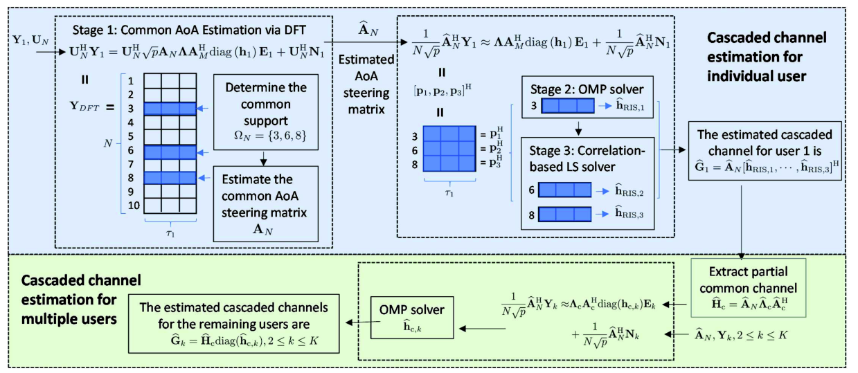
Due to the large number of antennas at the BS, the discrete Fourier transform (DFT) approach can be applied efficiently for AoA estimation from $\mathbf{Y}_{1}$ in (4). We first present the asymptotic properties of $\mathbf{A}_{N}$ in the following lemmas, whose proofs are provided in Appendix A and Appendix B.

Lemma 1

When $N\rightarrow\infty$ , the following property holds

\lim_{N\rightarrow\infty}\frac{1}{N}\mathbf{a}_{N}^{\mathrm{H}}(\psi_{j})\mathbf{a}_{N}(\psi_{i})=\begin{cases}1&\psi_{j}=\psi_{i}\\ 0&\textrm{otherwise}\end{cases},

(16)

and $\mathbf{A}_{N}^{\mathrm{H}}\mathbf{A}_{N}=N\mathbf{I}_{L}$ , where $\mathbf{I}_{L}$ is the identity matrix of dimension $L\times L$ .

Lemma 2

When $N\rightarrow\infty$ , if the condition $\frac{d_{\mathrm{BS}}}{\lambda_{c}}\leq 1$ holds, then the DFT of $\mathbf{A}_{N}$ , i.e., $\mathbf{U}_{N}^{\mathrm{H}}\mathbf{A}_{N}$ , is a tall sparse matrix with one nonzero element in each column

\lim_{N\rightarrow\infty}[\mathbf{U}_{N}^{\mathrm{H}}\mathbf{A}_{N}]_{n_{l},l}\neq 0,\forall l,

where $\mathbf{U}_{N}$ is the normalized DFT matrix with $(n,m)$ -th entry $[\mathbf{U}_{N}]_{n,m}=\frac{1}{\sqrt{N}}e^{-\mathrm{i}\frac{2\pi}{N}(n-1)(m-1)}$ , and

n_{l}=\begin{cases}N\psi_{l}+1&\psi_{l}\in[0,\frac{d_{\mathrm{BS}}}{\lambda_{c}})\\ N+N\psi_{l}+1&\psi_{l}\in[-\frac{d_{\mathrm{BS}}}{\lambda_{c}},0)\end{cases}.

(17)

Based on Lemma 2, any two nonzero elements are not in the same row, i.e., $n_{l}\neq n_{i}$ for any $l\neq i$ .

Remark 1: It is observed from (17) that when $\psi_{l}\in[0,\frac{d_{\mathrm{BS}}}{\lambda_{c}})$ , the range of $n_{l}$ is $n_{l}\in\text{[}1,N\frac{d_{\mathrm{BS}}}{\lambda_{c}}+1)$ . When $\psi_{l}\in[-\frac{d_{\mathrm{BS}}}{\lambda_{c}},0)$ , we have $n_{l}\in[N-N\frac{d_{\mathrm{BS}}}{\lambda_{c}}+1,N+1)$ . In order to avoid ambiguous angles where the same $n_{l}$ corresponds to two AoAs, we much have $N\frac{d_{\mathrm{BS}}}{\lambda_{c}}+1\leq N-N\frac{d_{\mathrm{BS}}}{\lambda_{c}}+1$ , which leads to $d_{\mathrm{BS}}\leq\frac{\lambda_{c}}{2}$ . Therefore, $d_{\mathrm{BS}}$ should generally be restricted to be no larger than $\lambda_{c}/2$ to avoid AoA ambiguity.

Based on Lemma 2, matrix $\mathbf{U}_{N}^{\mathrm{H}}\mathbf{A}_{N}$ can be regarded as a row sparse matrix with full column rank. Thus, the DFT of $\mathbf{Y}_{1}$ , i.e., $\mathbf{Y}_{DFT}=\mathbf{U}_{N}^{\mathrm{H}}\mathbf{Y}_{1}=\sqrt{p}\mathbf{U}_{N}^{\mathrm{H}}\mathbf{A}_{N}\bm{\Lambda}\mathbf{A}_{M}^{\mathrm{H}}\mathrm{Diag}\left(\mathbf{h}_{1}\right)\mathbf{E}_{1}+\mathbf{U}_{N}^{\mathrm{H}}\mathbf{N}_{1}$ , is an asymptotic row sparse matrix with $L$ nonzero rows, each corresponding to one of the AoAs as shown in Fig. 2. Based on the above discussion, $\phi_{l}$ can be immediately estimated from the nonzero rows of $\mathbf{Y}_{DFT}$ . However, $N$ is finite in practice, and thus $N\psi_{l}$ is usually not an integer. Most of the power of $\mathbf{Y}_{DFT}$ will be concentrated on the $(\left\lfloor N\psi_{l}\right\rceil+1)$ -th or the $(N+\left\lfloor N\psi_{l}\right\rceil+1)$ -th row, while the remaining power leaks to nearby rows. This is known as the power leakage effect [16, 17, 18, 19]. Due to the fact that the resolution of the DFT is $1/N$ , there exists a mismatch between the discrete estimated angle and the real continuous angle. To improve the angle estimation accuracy, we adopt an angle rotation operation to compensate for the mismatch of the DFT [16, 17, 18].

The angle rotation matrices are defined as

\displaystyle\bm{\Phi}_{N}(\triangle\psi_{l})

\displaystyle=\mathrm{Diag}\{1,e^{\mathrm{i}\triangle\psi_{l}},\ldots,e^{\mathrm{i}(N-1)\triangle\psi_{l}}\},\forall l,

where $\triangle\psi_{l}\in[-\frac{\pi}{N},\frac{\pi}{N}]$ are the phase rotation parameters. Then, the angle rotation of $\mathbf{Y}_{1}$ for $\phi_{l}$ is defined as

\mathbf{Y}_{1,l}^{ro}=\bm{\Phi}_{N}^{\mathrm{H}}(\triangle\psi_{l})\mathbf{Y}_{1}.

(18)

The aim of the angle rotation in (18) is to rotate $\mathbf{A}_{N}$ in the angle domain such that there is no power leakage for estimating $\psi_{l}$ . For better illustration, we take $\mathbf{U}_{N}^{\mathrm{H}}\bm{\Phi}_{N}^{\mathrm{H}}(\triangle\psi_{l})\mathbf{A}_{N}$ as an example, whose $(n,l)$ -th element is calculated as

\displaystyle[\mathbf{U}_{N}^{\mathrm{H}}\bm{\Phi}_{N}^{\mathrm{H}}(\triangle\psi_{l})\mathbf{A}_{N}]_{n,l}

\displaystyle=\sqrt{\frac{1}{N}}\sum_{m=1}^{N}e^{-\mathrm{i}2\pi(m-1)(\psi_{l}+\frac{\triangle\psi_{l}}{2\pi}-\frac{n-1}{N})}.

It can be readily found that the channel power of $\psi_{l}$ is concentrated on the $n_{l}$ -th row without power leakage when the phase rotation parameter satisfies

\displaystyle\triangle\psi_{l}

\displaystyle=2\pi\left(\frac{n_{l}-1}{N}-\psi_{l}\right).

(19)

For $\mathbf{Y}_{1}$ , the optimal phase rotation parameter for $\psi_{l}$ can be found based on a one-dimensional search by solving the following problem

\displaystyle\triangle\psi_{l}=\mathrm{arg}\max_{\triangle\psi\in[-\frac{\pi}{N},\frac{\pi}{N}]}

\displaystyle||[\mathbf{U}_{N}]_{:,n_{l}}^{\mathrm{H}}\bm{\Phi}_{N}^{\mathrm{H}}(\triangle\psi)\mathbf{Y}_{1}||^{2}.

(20)

Fig. 3 is an example of the row sparse characteristic of $\mathbf{Y}_{DFT}$ and the Y-axis is the power of each row of $\mathbf{Y}_{DFT}$ . The cascaded channel of size $N=M=100$ contains one ( $L=1$ ) path between the BS and the RIS with $\phi=14^{\circ}$ . It can be seen from the blue curve that although the beam covers several points because of power leakage, we can locate the power peak of the beam, which can be utilized for initial AoA estimation. The orange curve demonstrates the effect of the optimal angle rotation for $\phi=14{}^{\circ}$ . It is obvious that more power is focused on $\phi=14{}^{\circ}$ , which makes the AoA estimation more accurate.

Algorithm 1 Common AoA Estimation

\mathbf{Y}_{1}

1: Calculate DFT:

\mathbf{Y}_{DFT}=\mathbf{U}_{N}^{\mathrm{H}}\mathbf{Y}_{1}

;

2: Calculate the power of each row:

\mathbf{z}(n)=||[\mathbf{Y}_{DFT}]_{n,:}||^{2},\forall n=1,2,\ldots,N

;

3: Find the rows with the power peak:

(\Omega_{N},\widehat{L})=\Gamma(\mathbf{z})

, where

\Omega_{N}=\{n_{l},l=1,\cdots,\widehat{L}\}

;

4: Calculate the optimal angle rotation parameters

\{\triangle\widehat{\psi}_{l}\}_{l=1}^{\widehat{L}}

via (20);

5: Estimate AOAs for

1\leq l\leq\widehat{L}

\displaystyle\widehat{\phi}_{l}=\begin{cases}\arccos\left(\frac{\lambda_{c}(n_{l}-1)}{d_{\mathrm{BS}}N}-\frac{\lambda_{c}\triangle\psi_{l}}{2\pi d_{\mathrm{BS}}}\right),&n_{l}\leq N\frac{d_{\mathrm{BS}}}{\lambda_{c}}\\ \arccos\left(\frac{\lambda_{c}(n_{l}-N-1)}{d_{\mathrm{BS}}N}-\frac{\lambda_{c}\triangle\psi_{l}}{2\pi d_{\mathrm{BS}}}\right),&n_{l}>N\frac{d_{\mathrm{BS}}}{\lambda_{c}}\end{cases}.

(21)

\{\widehat{\phi}_{l}\}_{l=1}^{\widehat{L}}

Algorithm 1 summarizes the estimation of the common AoAs. After calculating the sum power of each row of $\mathbf{Y}_{DFT}$ in Step 2, we find the set of row indexes with peak power in Step 3. $\Gamma(\mathbf{z})$ denotes the operation of finding the indicies with peak power in vector $\mathbf{z}$ , $\Omega_{N}=\{n_{l},l=1,\cdots,\widehat{L}\}$ is a set to collect the indicies of the non-zero rows, and $\widehat{L}$ is the number of non-zero rows. We note that $\widehat{L}$ is the estimated number of the propagation paths between the BS and the RIS, and also the estimated number of common AoAs. For each $n_{l}$ , Problem (20) is solved to find the optimal angle rotation parameter in Step 4. Finally, the common AOAs are estimated in Step 5.

III-B2 Estimation of the cascaded AoD cosines and gains

With the estimated AoAs $\{\widehat{\phi}_{l}\}_{l=1}^{\widehat{L}}$ from Algorithm 1, we obtain the estimated steering matrix $\mathbf{\widehat{A}}_{N}=[\mathbf{a}_{N}(\widehat{\psi}_{1}),\ldots,\mathbf{a}_{N}(\widehat{\psi}_{\widehat{L}})]\in\mathbb{C}^{N\times\widehat{L}}$ . Based on the orthogonality of the massive steering matrix, i.e., $\mathbf{\widehat{A}}_{N}^{\mathrm{H}}\mathbf{A}_{N}\approx N\mathbf{I}_{L}$ due to Lemma 1, the measurement matrix $\mathbf{Y}_{1}$ can be projected onto the common AoA steering matrix subspace as

	$\displaystyle\frac{1}{N\sqrt{p}}\mathbf{\widehat{A}}_{N}^{\mathrm{H}}\mathbf{Y}_{1}$	$\displaystyle\approx\bm{\Lambda}\mathbf{A}_{M}^{\mathrm{H}}\mathrm{Diag}\left(\mathbf{h}_{1}\right)\mathbf{E}_{1}+\frac{1}{N\sqrt{p}}\mathbf{\widehat{A}}_{N}^{\mathrm{H}}\mathbf{N}_{1}$
		$\displaystyle={\bf H}_{\mathrm{RIS}}^{\mathrm{H}}\mathbf{E}_{1}+\frac{1}{N\sqrt{p}}\mathbf{\widehat{A}}_{N}^{\mathrm{H}}\mathbf{N}_{1},$		(22)

where ${\bf H}_{\mathrm{RIS}}=\mathrm{Diag}\left(\mathbf{h}_{1}^{*}\right)\mathbf{A}_{M}\bm{\Lambda}^{\mathrm{H}}$ . Based on (12b) and (12c), the $l$ -th column of ${\bf H}_{\mathrm{RIS}}$ is given by

{\bf h}_{\mathrm{RIS},l}=\mathrm{Diag}\{{\bf h}_{1}^{*}\}\mathbf{a}_{M}(\omega_{l})\alpha_{l}^{*},

(23)

where ${\bf H}_{\mathrm{RIS}}=[\mathbf{h}_{\mathrm{RIS},1},\cdots,\mathbf{h}_{\mathrm{RIS},L}]$ . We claim that ${\bf h}_{\mathrm{RIS},l}$ can be estimated by transforming each row of (22) into a sparse signal recovery problem. In particular, define $\frac{1}{N\sqrt{p}}\mathbf{\widehat{A}}_{N}^{\mathrm{H}}\mathbf{Y}_{1}=[\mathbf{p}_{1},\ldots,\mathbf{p}_{L}]^{\mathrm{H}}$ , where

	$\displaystyle\mathbf{p}_{l}$	$\displaystyle=\mathbf{E}_{1}^{\mathrm{H}}\mathbf{h}_{\mathrm{RIS},l}+\mathbf{n}_{\mathrm{noise}}\in\mathbb{C}^{\tau_{1}\times 1}$
		$\displaystyle=\mathbf{E}_{1}^{\mathrm{H}}\mathrm{Diag}\{\mathbf{a}_{M}(\omega_{l})\}{\bf h}_{1}^{}\alpha_{l}^{}+\mathbf{n}_{\mathrm{noise}}$
		$\displaystyle=\mathbf{E}_{1}^{\mathrm{H}}\mathrm{Diag}\{\mathbf{a}_{M}(\omega_{l})\}\mathbf{A}_{M,1}^{}\bm{\beta}_{1}^{}\alpha_{l}^{*}+\mathbf{n}_{\mathrm{noise}}$
		$\displaystyle=\mathbf{E}_{1}^{\mathrm{H}}\left[\begin{array}[]{ccc}\mathbf{a}_{M}\left(\omega_{l}-\varphi_{1,1}\right)&\cdots&\mathbf{a}_{M}\left(\omega_{l}-\varphi_{1,J_{1}}\right)\end{array}\right]\bm{\beta}_{1}^{}\alpha_{l}^{}+\mathbf{n}_{\mathrm{noise}}$

with $\mathbf{n}_{\mathrm{noise}}$ representing the corresponding noise vector. To extract the cascaded directional cosine $\{\omega_{l}-\varphi_{1,j}\}_{j=1}^{J_{1}}$ and gains $\bm{\beta}_{1}^{*}\alpha_{l}^{*}$ from $\mathbf{p}_{l}$ , (III-B2) can be approximated by using the VAD representation as

\displaystyle\mathbf{p}_{l}

\displaystyle=\mathbf{E}_{1}^{\mathrm{H}}\mathbf{A}\mathbf{b}_{l}+\mathbf{n}_{\mathrm{noise}},

(25)

where $\mathbf{A}\in\mathbb{C}^{M\times D}(M\ll D)$ is an overcomplete dictionary matrix, each column of which represents the array steering vector for possible values of $\omega_{l}-\varphi_{1,j}$ . Since $\omega_{l}-\varphi_{1,j}\in[-2\frac{d_{\mathrm{RIS}}}{\lambda_{c}},2\frac{d_{\mathrm{RIS}}}{\lambda_{c}}]$ , $\mathbf{A}$ can be constructed as

\displaystyle\mathbf{A}=\biggl[\mathbf{a}_{M}(-2\frac{d_{\mathrm{RIS}}}{\lambda_{c}}),\mathbf{a}_{M}((-2+\frac{4}{D})\frac{d_{\mathrm{RIS}}}{\lambda_{c}}),\ldots,.\mathbf{a}_{M}((2-\frac{4}{D})\frac{d_{\mathrm{RIS}}}{\lambda_{c}})\biggr].

(26)

Recall that $\bm{\beta}_{1}=[\beta_{1,1},\ldots,\beta_{1,J_{1}}]^{\mathrm{T}}$ in (14b), $\mathbf{b}_{l}\in\mathbb{C}^{D\times 1}$ is then a sparse vector with $J_{1}$ cascaded gains $\{\alpha_{l}^{*}\beta_{1,j}^{*}\}_{j=1}^{J_{1}}$ as nonzero elements. Equation (25) can be cast as a sparse signal recovery problem that can be solved using CS techniques, such as OMP. Note that the phase shift matrix $\mathbf{E}_{1}$ in (25) will be designed for better estimation in Section IV. It has been proved that $\tau_{1}\geq 8J_{1}-2$ measurements are sufficient to recover a $J_{1}$ -sparse complex-valued signal vector [20].

However, if OMP is used $L$ times for solving $\mathbf{p}_{l}(1\leq l\leq L)$ , we need to estimate $J_{1}L$ independent sparse variables with high complexity. In order to reduce the complexity, we exploit the following scaling property. Specifically, we observe from (23) that there is an angle and gain scaling between the cascaded multipaths formed by different AoDs $\{\omega_{l}\}_{l=1}^{L}$ from the RIS. That is, there is the following relationship between ${\bf h}_{\mathrm{RIS},l}$ and ${\bf h}_{\mathrm{RIS},r}$ for $1\leq l,r\leq L$ :

	$\displaystyle{\bf h}_{\mathrm{RIS},l}$	$\displaystyle=\mathrm{Diag}\{\mathbf{a}_{M}(\omega_{l}-\omega_{r})\}\mathrm{Diag}\{{\bf h}_{1}^{}\}\mathbf{a}_{M}(\omega_{r})\alpha_{r}^{}\frac{\alpha_{l}^{}}{\alpha_{r}^{}}$
		$\displaystyle=\mathrm{Diag}\{\mathbf{a}_{M}(\omega_{l}-\omega_{r})\}{\bf h}_{\mathrm{RIS},r}\frac{\alpha_{l}^{}}{\alpha_{r}^{}}.$		(27)

Equation (27) is called the angle-gain scaling property, which implies that ${\bf h}_{\mathrm{RIS},l}$ for all $l$ can be represented by one arbitrary ${\bf h}_{\mathrm{RIS},r}$ . Let


$\displaystyle\triangle\omega_{l}$	$\displaystyle=\omega_{l}-\omega_{r},$	(28a)
$\displaystyle x_{l}$	$\displaystyle=\frac{\alpha_{l}^{}}{\alpha_{r}^{}}.$	(28b)

Equation (27) is then re-expressed as ${\bf h}_{\mathrm{RIS},l}=\mathrm{Diag}\{{\bf h}_{\mathrm{RIS},r}\}\mathbf{a}_{M}(\triangle\omega_{l})x_{l}$ . Denote the estimate of ${\bf h}_{\mathrm{RIS},r}$ as $\widehat{{\bf h}}_{\mathrm{RIS},r}$ obtained from (25) using OMP. Further defining $\mathbf{z}_{l}(\triangle\omega_{l})=\mathbf{E}_{1}^{\mathrm{H}}\mathrm{Diag}\{\widehat{{\bf h}}_{\mathrm{RIS},r}\}\mathbf{a}_{M}(\triangle\omega_{l})$ , (III-B2) can be rewritten as

\mathbf{p}_{l}=\mathbf{z}_{l}(\triangle\omega_{l})x_{l}+\mathbf{n}_{\mathrm{noise}}.

(29)

It is observed from (29) that only two variables $\triangle\omega_{l}$ and $x_{l}$ need to be estimated. Since $\triangle\omega_{l}\in[-2\frac{d_{\mathrm{RIS}}}{\lambda_{c}},2\frac{d_{\mathrm{RIS}}}{\lambda_{c}}]$ , $\triangle\omega_{l}$ can then be estimated via a simple correlation-based scheme

\triangle\widehat{\omega}_{l}=\mathrm{arg}\max_{\triangle\omega\in[-2\frac{d_{\mathrm{RIS}}}{\lambda_{c}},2\frac{d_{\mathrm{RIS}}}{\lambda_{c}}]}\left|\left\langle\mathbf{p}_{l},\mathbf{z}_{l}(\triangle\omega)\right\rangle\right|.

(30)

The parameter $x_{l}$ can be found as the solution of the LS problem $\min_{x}||\mathbf{p}_{l}-\mathbf{z}_{l}(\triangle\widehat{\omega}_{l})x||_{2}$ :

\widehat{x}_{l}=(\mathbf{z}_{l}^{\mathrm{H}}(\triangle\widehat{\omega}_{l})\mathbf{z}_{l}(\triangle\widehat{\omega}_{l}))^{-1}\mathbf{z}_{l}^{\mathrm{H}}(\triangle\widehat{\omega}_{l})\mathbf{p}_{l}.

(31)

Let $\widehat{{\bf h}}_{\mathrm{RIS},l}=\mathrm{Diag}\{\widehat{{\bf h}}_{\mathrm{RIS},r}\}\mathbf{a}_{M}(\triangle\widehat{\omega}_{l})\widehat{x}_{l},(1\leq l\leq L,l\neq r)$ , so that the final estimated cascaded channel of user $1$ is given by

\widehat{\mathbf{G}}_{1}=\mathbf{\widehat{A}}_{N}\widehat{{\bf H}}_{\mathrm{R\mathrm{IS}}}^{\mathrm{H}},

(32)

where $\widehat{{\bf H}}_{\mathrm{RIS}}=[\widehat{{\bf h}}_{\mathrm{RIS},1},\cdots,\widehat{{\bf h}}_{\mathrm{RIS},L}]$ .

Algorithm 2 summarizes the complete estimation of $\mathbf{G}_{1}$ . The common AoA steering matrix $\mathbf{A}_{N}$ is estimated by using the DFT and the angle rotation techniques in Stage 1. In Stage 2 consisting of Steps 3-12, OMP is used to estimate ${\bf h}_{\mathrm{RIS},r}$ . Here, $r$ is determined according to Problem (35) such that the SNR of $\mathbf{p}_{r}$ is the maximum value among $\{\mathbf{p}_{l}\}_{l=1}^{L}$ (assuming they have the same noise power) for better estimation accuracy for the OMP method. The remaining ${\bf h}_{\mathrm{RIS},l}$ ( $1\leq l\leq\widehat{L}$ and $l\neq r$ ) are estimated using the simple LS method and correlation-based scheme in Stage 3 shown in Steps 13-16. Finally, we obtain the estimate $\widehat{\mathbf{G}}_{1}=\mathbf{\widehat{A}}_{N}[\widehat{{\bf h}}_{\mathrm{RIS},1},\cdots,\widehat{{\bf h}}_{\mathrm{RIS},\widehat{L}}]^{\mathrm{H}}$ . The flow chart of Algorithm 2 is shown in Fig. 2.

We emphasize that the cascaded AoD cosines and cascaded gains can also been obtained in Algorithm 2, which facilitates the cascaded channel estimation of other users in the next subsection. In particular, the cascaded AoD cosines and cascaded gains from $\widehat{{\bf h}}_{\mathrm{RIS},r}$ in Step 12 are given by


$\displaystyle[\mathbf{a}_{M}(\widehat{\omega_{r}-\varphi_{1,1}})\cdots\mathbf{a}_{M}(\widehat{\omega_{r}-\varphi_{1,\widehat{J}_{1}}})]$	$\displaystyle=\mathbf{A}_{(:,\Omega_{i-1})},$	(33a)
$\displaystyle\widehat{\bm{\beta}_{1}^{}\alpha_{r}^{}}$	$\displaystyle=\mathbf{b}_{i-1}.$	(33b)

Based on (28) and (33), the cascaded AoD cosines and cascaded gains from $\widehat{{\bf h}}_{\mathrm{RIS},l}$ ( $1\leq l\leq\widehat{L}$ and $l\neq r$ ) in Step 16 are given by


$\displaystyle[\mathbf{a}_{M}(\widehat{\omega_{l}-\varphi_{1,1}})\cdots\mathbf{a}_{M}(\widehat{\omega_{l}-\varphi_{1,\widehat{J}_{1}}})]$	$\displaystyle=\mathrm{Diag}\{\mathbf{a}_{M}(\triangle\widehat{\omega}_{l})\}\mathbf{A}_{(:,\Omega_{i-1})},$	(34a)
$\displaystyle\widehat{\bm{\beta}_{1}^{}\alpha_{l}^{}}$	$\displaystyle=\widehat{\bm{\beta}_{1}^{}\alpha_{r}^{}}\widehat{x}_{l}.$	(34b)

Algorithm 2 estimates $L$ AoAs in Stage 1, $J_{1}$ cascaded AoD cosines and $J_{1}$ cascaded gains in (33), and $2L-2$ scaling parameters in Step 14 and Step 15. Therefore, Algorithm 2 uses a total of $\tau_{1}\geq 8J_{1}-2$ time slots to estimate $3L+2J_{1}-2$ parameters to recover channel $\mathbf{G}_{1}$ of dimension $N\times M$ . Note that the number of time slots required is not related to $L$ , which evidences the advantage of our proposed estimation method.

Algorithm 2 DFT-OMP-based Estimation of

\mathbf{G}_{1}

\mathbf{Y}_{1}

\mathbf{A}

1: Stage 1: Return estimated common AoA steering matrix

\mathbf{\widehat{A}}_{N}

and

\widehat{L}

using Algorithm 1.

2: Calculate

[\mathbf{p}_{1},\ldots,\mathbf{p}_{\widehat{L}}]=\frac{1}{N\sqrt{p}}\mathbf{Y}_{1}^{\mathrm{H}}\mathbf{\widehat{A}}_{N}

3: Stage 2: Estimate

{\bf h}_{\mathrm{RIS},r}

from

\mathbf{p}_{r}

using the OMP algorithm, where

r

is determined according to

r=\mathrm{arg}\max_{1\leq i\leq\widehat{L}}||\mathbf{p}_{i}||^{2}.

(35)

4: Calculate equivalent dictionary

\mathbf{D}=\mathbf{E}_{1}^{\mathrm{H}}\mathbf{A}

5: Initialize

\Omega_{0}=\emptyset

\mathbf{r}_{0}=\mathbf{p}_{r}

i=1

6: repeat

d_{i}=\mathrm{arg}\max_{d=1,2,\ldots,D}|\mathbf{D}_{(:,d)}^{\mathrm{H}}\mathbf{r}_{i-1}|.

\Omega_{i}=\Omega_{i-1}\cup d_{i}.

9: LS solution:

\mathbf{b}_{i}=(\mathbf{D}_{(:,\Omega_{i})}^{\mathrm{H}}\mathbf{D}_{(:,\Omega_{i})})^{-1}\mathbf{D}_{(:,\Omega_{i})}^{\mathrm{H}}\mathbf{p}_{r}.

10:

\mathbf{r}_{i}=\mathbf{p}_{r}-\mathbf{D}_{(:,\Omega_{i})}\mathbf{b}_{i}

11:

i=i+1

12: until

||\mathbf{r}_{i-1}||_{2}\leq

threshold.

13: Obtain the estimates:


		$\displaystyle\widehat{J}_{1}=i-1,$		(36a)
		$\displaystyle\widehat{{\bf h}}_{\mathrm{RIS},r}=\mathbf{A}_{(:,\Omega_{i-1})}\mathbf{b}_{i-1}.$		(36b)

14: Stage 3: Estimate

{\bf h}_{\mathrm{RIS},l}

from

\mathbf{p}_{l}

for

1\leq l\leq\widehat{L}

and

l\neq r

15: Calculate

\triangle\widehat{\omega}_{l}

according to (30).

16: Calculate

\widehat{x}_{l}

according to (31).

17: Obtain the estimates for

1\leq l\leq\widehat{L}

and

l\neq r

\displaystyle\widehat{{\bf h}}_{\mathrm{RIS},l}=\mathrm{Diag}\{\widehat{{\bf h}}_{\mathrm{RIS},r}\}\mathbf{a}_{M}(\triangle\widehat{\omega}_{l})\widehat{x}_{l}.

(37)

17:

\widehat{\mathbf{G}}_{1}=\mathbf{\widehat{A}}_{N}[\widehat{{\bf h}}_{\mathrm{RIS},1},\cdots,\widehat{{\bf h}}_{\mathrm{RIS},\widehat{L}}]^{\mathrm{H}}

III-C Channel Estimation for Other Users in the First Coherence Block

Algorithm 2 can also be used for the channel estimation of the other users, where Stage 1 can be omitted because all users share the common AoA steering matrix $\mathbf{\widehat{A}}_{N}$ . In addition to $\mathbf{\widehat{A}}_{N}$ , all users also share the common matrices $\bm{\Lambda}$ and $\mathbf{A}_{M}$ in their channel matrices $\mathbf{G}_{k},\forall k$ . Note that for the cascaded channel $\mathbf{G}_{k}=\mathbf{H}\mathrm{Diag}(\mathbf{h}_{k}),2\leq k\leq K$ in (3), we might expect that if the common channel $\mathbf{H}$ is known, channel $\mathbf{h}_{k}$ can be readily estimated using a sparse signal recovery problem. However, it is intractable to obtain $\mathbf{H}$ from the estimated cascaded channel $\widehat{\mathbf{G}}_{1}$ due to the coupling of angles $\cos(\theta_{l})-\cos(\vartheta_{1,j})$ and channel gains $\alpha_{l}\beta_{1,j}$ with each cascaded subpath of user $1$ . However, we can construct a substitute for $\mathbf{H}$ (denoted by $\mathbf{H}_{\mathrm{c}}$ ) by only using $\widehat{\mathbf{G}}_{1}$ . The substitute $\mathbf{H}_{\mathrm{c}}$ contains reparameterized information about $\mathbf{H}$ . Then, (3) can be rewritten as

\mathbf{G}_{k}=\mathbf{H}_{\mathrm{c}}\mathrm{Diag}(\mathbf{h}_{\mathrm{c},k}),2\leq k\leq K,

(38)

where $\mathbf{h}_{\mathrm{c},k}$ is the corresponding reparameterized CSI of $\mathbf{h}_{k}$ . In the following, we first construct $\mathbf{H}_{\mathrm{c}}$ based on the estimated channel information from Algorithm 2 and then estimate the reparameterized channel information $\mathbf{h}_{\mathrm{c},k}$ .

III-C1 Construction of $\mathbf{H}_{\mathrm{c}}$

In the following, we show how to construct $\mathbf{H}_{\mathrm{c}}$ by exploiting the structure of $\widehat{\mathbf{G}}_{1}$ . In particular, (11) is reformulated as

$\displaystyle\mathbf{H}$	$\displaystyle=\mathbf{A}_{N}\bm{\Lambda}\mathbf{A}_{M}^{\mathrm{H}}$
	$\displaystyle=\mathbf{A}_{N}\frac{1}{\overline{\beta}}\bm{\Lambda}_{\mathrm{c}}\mathbf{A}_{\mathrm{c}}^{\mathrm{H}}\mathrm{Diag}(\mathbf{a}_{M}(\overline{\varphi}))$
	$\displaystyle=\frac{1}{\overline{\beta}}\mathbf{H}_{\mathrm{c}}\mathrm{Diag}\left(\mathbf{a}_{M}(\overline{\varphi})\right),$	(39)

with


$\displaystyle\mathbf{H}_{\mathrm{c}}$	$\displaystyle=\mathbf{A}_{N}\bm{\Lambda}_{\mathrm{c}}\mathbf{A}_{\mathrm{c}}^{\mathrm{H}},$	(40a)
$\displaystyle\bm{\Lambda}_{\mathrm{c}}$	$\displaystyle=\overline{\beta}\bm{\Lambda},$	(40b)
$\displaystyle\mathbf{A}_{\mathrm{c}}$	$\displaystyle=\mathrm{Diag}(\mathbf{a}_{M}(\overline{\varphi}))\mathbf{A}_{M},$	(40c)
$\displaystyle\overline{\varphi}$	$\displaystyle=-\frac{1}{J_{1}}\sum_{j=1}^{J_{1}}\varphi_{1,j},$	(40d)
$\displaystyle\overline{\beta}$	$\displaystyle=\frac{1}{J_{1}}\mathbf{1}_{J_{1}}^{\mathrm{T}}\bm{\beta}_{1},$	(40e)

where $\mathbf{1}_{J_{1}}$ is an all-one vector with dimension $J_{1}\times 1$ , and $\bm{\beta}_{1}$ is defined in (14b).

Using (12b), (28b) and (40e), $\bm{\Lambda}_{\mathrm{c}}$ in (40b) can be re-expressed as


$\displaystyle\bm{\Lambda}_{\mathrm{c}}$	$\displaystyle=\overline{\beta}\bm{\Lambda}$
	$\displaystyle=\overline{\beta}\mathrm{Diag}(\alpha_{1},\ldots,\alpha_{L})$
	$\displaystyle=\left[\overline{\beta}^{}\alpha_{r}^{}\mathrm{Diag}(x_{1},\ldots,x_{L})\right]^{*}$	(41a)
	$\displaystyle=\left[\frac{1}{J_{1}}\mathbf{1}_{J_{1}}^{\mathrm{T}}\bm{\beta}_{1}^{}\alpha_{r}^{}\mathrm{Diag}(x_{1},\ldots,x_{L})\right]^{*},$	(41b)

where the estimate of $\bm{\beta}_{1}^{*}\alpha_{r}^{*}$ is given in (33b), and the estimate of $[x_{1},x_{2},\ldots,x_{L}]$ is given in (31). Then, the estimate of $\bm{\Lambda}_{\mathrm{c}}$ is obtained as

\widehat{\bm{\Lambda}}_{\mathrm{c}}=\left[\frac{1}{J_{1}}\mathbf{1}_{J_{1}}^{\mathrm{T}}\widehat{\bm{\beta}_{1}^{*}\alpha_{r}^{*}}\mathrm{Diag}([\widehat{x}_{1},\ldots,\widehat{x}_{\widehat{L}}])\right]^{*}.

(42)

For $\mathbf{A}_{\mathrm{c}}$ , by substituting (12c), (28a) and (40d) into (40c), we have


	$\displaystyle\mathbf{A}_{\mathrm{c}}$	$\displaystyle=\mathrm{Diag}(\mathbf{a}_{M}(\overline{\varphi}))\mathbf{A}_{M}$
		$\displaystyle=\mathrm{Diag}(\mathbf{a}_{M}(\overline{\varphi}))[\mathbf{a}_{M}(\omega_{1}),\ldots,\mathbf{a}_{M}(\omega_{L})]$
		$\displaystyle=\mathrm{Diag}(\mathbf{a}_{M}(\omega_{r}+\overline{\varphi}))[\mathbf{a}_{M}(\triangle\omega_{1}),\ldots,\mathbf{a}_{M}(\triangle\omega_{L})]$
		$\displaystyle=\mathrm{Diag}(\mathbf{a}_{M}(\omega_{r}-\frac{1}{J_{1}}\sum_{j=1}^{J_{1}}\varphi_{1,j}))[\mathbf{a}_{M}(\triangle\omega_{1}),\ldots,\mathbf{a}_{M}(\triangle\omega_{L})]$
		$\displaystyle=\mathrm{Diag}(\mathbf{a}_{M}(\frac{1}{J_{1}}\sum_{j=1}^{J_{1}}(\omega_{r}-\varphi_{1,j})))[\mathbf{a}_{M}(\triangle\omega_{1}),\ldots,\mathbf{a}_{M}(\triangle\omega_{L})],$

where the estimate of $\{\omega_{r}-\varphi_{1,j}\}_{j=1}^{J_{1}}$ and $\{\triangle\omega_{l}\}_{l=1}^{L}$ are given by (30) and (33a), respectively. Then, we can obtain the estimate of $\mathbf{A}_{\mathrm{c}}$ as

	$\displaystyle\widehat{\mathbf{A}}_{\mathrm{c}}=$	$\displaystyle\mathrm{Diag}(\mathbf{a}_{M}(\frac{1}{\widehat{J}_{1}}\sum_{j=1}^{\widehat{J}_{1}}(\widehat{\omega_{r}-\varphi_{1,j}})))[\mathbf{a}_{M}((\triangle\widehat{\omega}_{1}),\cdots\mathbf{a}_{M}(\triangle\widehat{\omega}_{\widehat{L}})]$
	$\displaystyle=$	$\displaystyle\mathrm{Diag}(\mathbf{a}_{M}(\widehat{\omega_{r}+\overline{\varphi}}))[\mathbf{a}_{M}((\triangle\widehat{\omega}_{1}),\cdots\mathbf{a}_{M}(\triangle\widehat{\omega}_{\widehat{L}})].$		(44)

With $\widehat{\mathbf{A}}_{N}$ , (42) and (44), the estimate of $\mathbf{H}_{\mathrm{c}}$ is given by $\widehat{\mathbf{H}}_{\mathrm{c}}=\widehat{\mathbf{A}}_{N}\widehat{\bm{\Lambda}}_{\mathrm{c}}\widehat{\mathbf{A}}_{\mathrm{c}}^{\mathrm{H}}$ .

III-C2 Estimation of reparameterized CSI $\mathbf{h}_{\mathrm{c},k}$

In this subsection, we discuss how to use the reparameterized common channel $\mathbf{H}_{\mathrm{c}}$ to help the channel estimation of other users with low pilot overhead. In particular, by substituting $\mathbf{H}=\frac{1}{\overline{\beta}}\mathbf{H}_{\mathrm{c}}\mathrm{Diag}(\mathbf{a}_{M}(\overline{\varphi}))$ in (39) into (3), we have

$\displaystyle\mathbf{G}_{k}$	$\displaystyle=\mathbf{H}\mathrm{Diag}(\mathbf{h}_{k})$
	$\displaystyle=\frac{1}{\overline{\beta}}\mathbf{H}_{\mathrm{c}}\mathrm{Diag}\left(\mathbf{a}_{M}(\overline{\varphi})\right)\mathrm{Diag}(\mathbf{h}_{k})$
	$\displaystyle=\frac{1}{\overline{\beta}}\mathbf{H}_{\mathrm{c}}\mathrm{Diag}\left(\mathrm{Diag}\left(\mathbf{a}_{M}(\overline{\varphi})\right)\mathbf{h}_{k}\right)$
	$\displaystyle=\mathbf{H}_{\mathrm{c}}\mathrm{Diag}(\mathbf{h}_{\mathrm{c},k}),$	(45)

where

\mathbf{h}_{\mathrm{c},k}=\frac{1}{\overline{\beta}}\mathrm{Diag}\left(\mathbf{a}_{M}(\overline{\varphi})\right)\mathbf{h}_{k}

(46)

contains reparameterized CSI of $\mathbf{h}_{k}$ .

Similar to (22), $\mathbf{Y}_{k}$ in (4) is first projected onto the common AoA steering matrix subspace as

	$\displaystyle\frac{1}{N\sqrt{p}}\mathbf{\widehat{A}}_{N}^{\mathrm{H}}\mathbf{Y}_{k}$	$\displaystyle=\frac{1}{N\sqrt{p}}\mathbf{\widehat{A}}_{N}^{\mathrm{H}}(\sqrt{p}\mathbf{H}_{\mathrm{c}}\mathrm{Diag}(\mathbf{h}_{\mathrm{c},k})\mathbf{E}_{k}+\mathbf{N}_{k})$
		$\displaystyle\approx\bm{\Lambda}_{\mathrm{c}}\mathbf{A}_{\mathrm{c}}^{\mathrm{H}}\mathrm{Diag}(\mathbf{h}_{\mathrm{c},k})\mathbf{E}_{k}+\frac{1}{N\sqrt{p}}\mathbf{\widehat{A}}_{N}^{\mathrm{H}}\mathbf{N}_{k}.$		(47)

Recall that $\mathbf{E}_{k}=[\mathbf{e}_{1},\ldots,\mathbf{e}_{\tau_{k}}]$ in (5a). By vectorizing (47) and defining $\mathbf{z}_{k}=\mathrm{vec}(\frac{1}{N\sqrt{p}}\mathbf{\widehat{A}}_{N}^{\mathrm{H}}\mathbf{Y}_{k})\in\mathbb{C}^{\tau_{k}L\times 1}$ , we have

	$\displaystyle\mathbf{z}_{k}$	$\displaystyle=\left[\begin{array}[]{c}\bm{\Lambda}_{\mathrm{c}}\mathbf{A}_{\mathrm{c}}^{\mathrm{H}}\mathrm{Diag}(\mathbf{h}_{\mathrm{c},k})\mathbf{e}_{1}\\ \vdots\\ \bm{\Lambda}_{\mathrm{c}}\mathbf{A}_{\mathrm{c}}^{\mathrm{H}}\mathrm{Diag}(\mathbf{h}_{\mathrm{c},k})\mathbf{e}_{\tau_{k}}\end{array}\right]+\mathbf{n}_{\mathrm{noise}}$
		$\displaystyle=\mathbf{Z}_{k}\mathbf{h}_{\mathrm{c},k}+\mathbf{n}_{\mathrm{noise}},$		(51)

where $\mathbf{n}_{\mathrm{noise}}$ represents the corresponding noise and

\mathbf{Z}_{k}=\left[\begin{array}[]{c}\bm{\Lambda}_{\mathrm{c}}\mathbf{A}_{\mathrm{c}}^{\mathrm{H}}\mathrm{Diag}\left(\mathbf{e}_{1}\right)\\ \vdots\\ \bm{\Lambda}_{\mathrm{c}}\mathbf{A}_{\mathrm{c}}^{\mathrm{H}}\mathrm{Diag}\left(\mathbf{e}_{\tau_{k}}\right)\end{array}\right].

(52)

By replacing $\mathbf{h}_{k}$ with $\mathbf{h}_{k}=\mathbf{A}_{M,k}\bm{\beta}_{k}$ from (13), $\mathbf{h}_{\mathrm{c},k}$ in (46) can be unfolded as

	$\displaystyle\mathbf{h}_{\mathrm{c},k}$	$\displaystyle=\frac{1}{\overline{\beta}}\mathrm{Diag}\left(\mathbf{a}_{M}(\overline{\varphi})\right)\mathbf{h}_{k}$
		$\displaystyle=\frac{1}{\overline{\beta}}[\mathbf{a}_{M}\left(\varphi_{k,1}+\overline{\varphi}\right)\cdots\mathbf{a}_{M}\left(\varphi_{k,J_{k}}+\overline{\varphi}\right)]\bm{\beta}_{k}.$		(53)

Since $\varphi_{k,1}+\overline{\varphi}\in[-2\frac{d_{\mathrm{RIS}}}{\lambda_{c}},2\frac{d_{\mathrm{RIS}}}{\lambda_{c}}]$ , (53) can be further approximated by using the VAD representation as

\displaystyle\mathbf{h}_{\mathrm{c},k}

\displaystyle=\mathbf{A}\mathbf{c}_{k},

(54)

where $\mathbf{A}$ is defined in (26), and $\mathbf{c}_{k}\in\mathbb{C}^{G\times 1}$ is a sparse vector with $J_{k}$ gains $\{\frac{1}{\overline{\beta}}\beta_{k,j}\}_{j=1}^{J_{k}}$ as the nonzero elements.

With (54), (51) can be approximated as a sparse signal recovery problem

\mathbf{z}_{k}=\mathbf{Z}_{k}\mathbf{A}\mathbf{c}_{k}+\mathbf{n}_{\mathrm{noise}}.

(55)

Note that $\mathbf{Z}_{k}$ is determined using (42) and (44). Hence, Problem (55) could be solved by using CS technique, such as OMP. Note that the phase shift vectors $\{\mathbf{e}_{t}\}_{t=1}^{\tau_{k}}$ in $\mathbf{Z}_{k}$ will be designed in Section IV to achieve high estimation accuracy.

Algorithm 3 summarizes the OMP-based estimation of $\mathbf{G}_{k},2\leq k\leq K$ . To effectively recover the $J_{k}$ -sparse signal $\mathbf{c}_{k}$ , the dimension of $\mathbf{z}_{k}\in\mathbb{C}^{\tau_{k}L\times 1}$ should satisfy the requirement $\tau_{k}L\geq 8J_{k}-2$ [20]. Thus, the pilot overhead required by user $k$ is $\tau_{k}\geq(8J_{k}-2)/L$ .

Algorithm 3 Estimation of

\mathbf{G}_{k},2\leq k\leq K

\mathbf{A}

\mathbf{Y}_{k},2\leq k\leq K

1: Return

\mathbf{\widehat{A}}_{N}

from Algorithm 1.

2: Construct

\widehat{\bm{\Lambda}}_{\mathrm{c}}

according to (42).

3: Construct

\widehat{\mathbf{A}}_{\mathrm{c}}

according to (44).

4: Calculate equivalent dictionary

\mathbf{R}=\mathbf{Z}_{k}\mathbf{A}

according to (52) with

\widehat{\bm{\Lambda}}_{\mathrm{c}}

and

\widehat{\mathbf{A}}_{\mathrm{c}}

5: for

2\leq k\leq K

6: Calculate

\mathbf{z}_{k}=\mathrm{vec}(\frac{1}{N\sqrt{p}}\mathbf{\widehat{A}}_{N}^{\mathrm{H}}\mathbf{Y}_{k})

7: Initialize

\Omega_{0}=\emptyset

\mathbf{r}_{0}=\mathbf{z}_{k}

i=1

8: repeat

d_{i}=\mathrm{arg}\max_{d=1,2,\ldots,D}|\mathbf{R}_{(:,d)}^{\mathrm{H}}\mathbf{r}_{i-1}|.

10:

\Omega_{i}=\Omega_{i-1}\cup d_{i}.

11: LS solution:

\mathbf{b}_{i}=(\mathbf{R}_{(:,\Omega_{i})}^{\mathrm{H}}\mathbf{R}_{(:,\Omega_{i})})^{-1}\mathbf{R}_{(:,\Omega_{i})}^{\mathrm{H}}\mathbf{p}_{r}.

12:

\mathbf{r}_{i}=\mathbf{p}_{r}-\mathbf{R}_{(:,\Omega_{i})}\mathbf{b}_{i}

13:

i=i+1

14: until

||\mathbf{r}_{i-1}||_{2}\leq

threshold.

15: Calculate the estimated reparameterized common channel

\widehat{\mathbf{H}}_{\mathrm{c}}=\widehat{\mathbf{A}}_{N}\widehat{\bm{\Lambda}}_{\mathrm{c}}\widehat{\mathbf{A}}_{\mathrm{c}}^{\mathrm{H}}

16: Obtain the estimates:


		$\displaystyle\widehat{\mathbf{h}}_{\mathrm{c},k}=\mathbf{A}_{(:,\Omega_{i-1})}\mathbf{b}_{i-1},$		(56a)
		$\displaystyle\widehat{\mathbf{G}}_{k}=\widehat{\mathbf{H}}_{\mathrm{c}}\mathrm{Diag}(\widehat{\mathbf{h}}_{\mathrm{c},k}).$		(56b)

17: end for

17:

\widehat{\mathbf{G}}_{k},2\leq k\leq K

We highlight the fact that the cascaded AoD cosines can also be obtained after $[\mathbf{a}_{M}(\widehat{\varphi_{k,1}+\overline{\varphi}})\cdots\\ \mathbf{a}_{M}(\widehat{\varphi_{k,J_{k}}+\overline{\varphi}})]=\mathbf{A}_{(:,\Omega_{i-1})}$ is determined from (53) when using OMP, which facilitates the cascaded channel estimation in the subsequent channel coherence blocks in the next subsection. In particular, the cascaded AoD cosines of user $k$ for $2\leq k\leq K$ and $1\leq l\leq L$ are given by

		$\displaystyle[\mathbf{a}_{M}(\widehat{\omega_{l}-\varphi_{k,1}})\cdots\mathbf{a}_{M}(\widehat{\omega_{l}-\varphi_{k,J_{k}}})]$
		$\displaystyle=\mathrm{Diag}(\mathbf{a}_{M}(\widehat{\omega_{l}+\overline{\varphi}}))[\mathbf{a}_{M}^{}(\widehat{\varphi_{k,1}+\overline{\varphi}})\cdots\mathbf{a}_{M}^{}(\widehat{\varphi_{k,J_{k}}+\overline{\varphi}})]$
		$\displaystyle=\mathrm{Diag}(\widehat{\mathbf{A}}_{\mathrm{c}(:,l)})[\mathbf{a}_{M}^{}(\widehat{\varphi_{k,1}+\overline{\varphi}})\cdots\mathbf{a}_{M}^{}(\widehat{\varphi_{k,J_{k}}+\overline{\varphi}})],$		(57)

where $\widehat{\mathbf{A}}_{\mathrm{c}(:,l)}$ is given in (44).

III-D Channel Estimation in the Remaining Coherence Blocks

The channel gains need to be re-estimated for the remaining channel coherence blocks as shown in Fig. 1. With knowledge of the angle information obtained in the first coherence block, only the cascaded channel gains need to be re-estimated.

For the remaining coherence blocks, the measurement matrix for user $k$ at the BS in (4) is considered again:

\mathbf{Y}_{k}=\sqrt{p}\mathbf{G}_{k}\mathbf{E}_{k}+\mathbf{N}_{k}\in\mathbb{C}^{N\times\tau_{k}}.

(58)

Following the same derivations as in (22) and (III-B2), we define $\frac{1}{N\sqrt{p}}\mathbf{\widehat{A}}_{N}^{\mathrm{H}}\mathbf{Y}_{k}=[\mathbf{q}_{k,1},\ldots,\mathbf{q}_{k,L}]^{\mathrm{H}}$ , where

\displaystyle\mathbf{q}_{k,l}

\displaystyle=\mathbf{E}_{k}^{\mathrm{H}}\mathbf{B}_{k,l}\bm{\beta}_{k}^{*}\alpha_{l}^{*}+\mathbf{n}_{\mathrm{noise}},

(59)

$\mathbf{B}_{k,l}=[\mathbf{a}_{M}(\omega_{l}-\varphi_{k,1})\cdots\mathbf{a}_{M}(\omega_{l}-\varphi_{k,J_{k}})]$ , and $\mathbf{n}_{\mathrm{noise}}$ represents the corresponding noise vector. Denote the estimate of $\mathbf{B}_{k,l}$ as $\widehat{\mathbf{B}}_{k,l}=[\mathbf{a}_{M}(\widehat{\omega_{l}-\varphi_{k,1}})\cdots\mathbf{a}_{M}(\widehat{\omega_{l}-\varphi_{k,J_{k}}})]$ obtained from (33a), (34a) for $k=1$ , and from (57) for $2\leq k\leq K$ in the first coherence block. Then the LS estimate of $\bm{\beta}_{k}^{*}\alpha_{l}^{*}$ is given by

\displaystyle\widehat{\bm{\beta}_{k}^{*}\alpha_{l}^{*}}

\displaystyle=(\widehat{\mathbf{B}}_{k,l}^{\mathrm{H}}\mathbf{E}_{k}\mathbf{E}_{k}^{\mathrm{H}}\widehat{\mathbf{B}}_{k,l})^{-1}\widehat{\mathbf{B}}_{k,l}^{\mathrm{H}}\mathbf{E}_{k}\mathbf{q}_{k,l},

(60)

Note that $\mathbf{E}_{k}^{\mathrm{H}}\widehat{\mathbf{B}}_{k,l}\in\mathbb{C}^{\tau_{k}\times J_{k}}$ must be a matrix with full row rank to ensure the feasibility of the pseudo inverse operation in (60), which means the pilot length must satisfy $\tau_{k}\geq J_{k}$ for user $k$ .

Define $\widehat{{\bf H}}_{\mathrm{RIS},k}=[\widehat{\mathbf{B}}_{k,1}\widehat{\bm{\beta}_{k}^{*}\alpha_{1}^{*}},\ldots,\widehat{\mathbf{B}}_{k,L}\widehat{\bm{\beta}_{k}^{*}\alpha_{L}^{*}}]$ . The uplink channel of the $k$ -th user can then be reconstructed using the updated cascaded channel gains obtained in this coherence block and the angle information obtained during the first coherence block as

\displaystyle\widehat{\mathbf{G}}_{k}=\mathbf{\widehat{A}}_{N}\widehat{{\bf H}}_{\mathrm{RIS},k}^{\mathrm{H}}.

(61)

IV Training reflection coefficient optimization

The performance of OMP-based channel estimation is positively related to the orthogonality of its equivalent dictionary. Therefore, in this section, we optimize the training phase shift matrices to generate approximately orthogonal equivalent dictionaries. Specifically, $\mathbf{E}_{k},\forall k\in\mathcal{K}$ are designed to improve the ability of OMP to recover the sparsest signals $\mathbf{b}_{l}$ and $\mathbf{c}_{k}$ from the sparse recovery problems $\mathbf{p}_{l}=\mathbf{E}_{1}^{\mathrm{H}}\mathbf{A}\mathbf{b}_{l}+\mathbf{n}_{\mathrm{noise}}$ in (25) and $\mathbf{z}_{k}=\mathbf{Z}_{k}\mathbf{A}\mathbf{c}_{k}+\mathbf{n}_{\mathrm{noise}}$ in (55), respectively. In the following, we first investigate the design of $\mathbf{E}_{1}$ in (25), and then extend the solution to the design of $\mathbf{E}_{k}$ $(2\leq k\leq K)$ .

Our approach is motivated by the theoretical work of [21] which shows that the sparse signal $\mathbf{b}_{l}$ can be recovered successfully by OMP only when the following condition holds:

||\mathbf{b}_{l}||_{0}\leq\frac{1}{2}\left(1+\frac{1}{\mu}\right),

(62)

where $\mu$ is the mutual coherence of the equivalent dictionary $\mathbf{D}=\mathbf{E}_{1}^{\mathrm{H}}\mathbf{A}$ defined by

\mu=\max_{i\neq j}\frac{|\mathbf{D}_{(:,i)}^{\mathrm{H}}\mathbf{D}_{(:,j)}|}{||\mathbf{D}_{(:,i)}||_{2}||\mathbf{D}_{(:,j)}||_{2}}.

(63)

The condition in (62) suggests that $\mathbf{D}$ should be as incoherent (orthogonal) as possible, which leads to the following design problem

	$\displaystyle\min_{\mathbf{E}_{1}}$	$\displaystyle\|\|\mathbf{D}^{\mathrm{H}}\mathbf{D}-\mathbf{I}_{D}\|\|_{F}^{2}$
	$\displaystyle\mathrm{s.t.}$	$\displaystyle\|[\mathbf{E}_{1}]_{m,n}\|=1,1\leq m\leq M,1\leq n\leq\tau_{1}.$		(64)

The solution for the unconstrained version of Problem (64) has been investigated in [22], and the method designed therein is extended to solve the constrained Problem (64) in [13]. Based on [13] and [22], we propose a more concise solution in the following. To begin, note that

	$\displaystyle\|\|\mathbf{D}^{\mathrm{H}}\mathbf{D}-\mathbf{I}_{D}\|\|_{F}^{2}$
$\displaystyle=$	$\displaystyle\mathrm{tr}\{\mathbf{D}^{\mathrm{H}}\mathbf{D}\mathbf{D}^{\mathrm{H}}\mathbf{D}-2\mathbf{D}^{\mathrm{H}}\mathbf{D}+\mathbf{I}_{D}\}$
$\displaystyle=$	$\displaystyle\mathrm{tr}\{\mathbf{D}\mathbf{D}^{\mathrm{H}}\mathbf{D}\mathbf{D}^{\mathrm{H}}-2\mathbf{D}\mathbf{D}^{\mathrm{H}}+\mathbf{I}_{\tau_{1}}\}+(D-\tau_{1})$
$\displaystyle=$	$\displaystyle\|\|\mathbf{D}\mathbf{D}^{\mathrm{H}}-\mathbf{I}_{\tau_{1}}\|\|_{F}^{2}+(D-\tau_{1}).$	(65)

Using (65), Problem (64) reduces to

	$\displaystyle\min_{\mathbf{E}_{1}}$	$\displaystyle\|\|\mathbf{D}\mathbf{D}^{\mathrm{H}}-\mathbf{I}_{\tau_{1}}\|\|_{F}^{2}=\|\|\mathbf{E}_{1}^{\mathrm{H}}\mathbf{A}\mathbf{A}^{\mathrm{H}}\mathbf{E}_{1}-\mathbf{I}_{\tau_{1}}\|\|_{F}^{2}$
	$\displaystyle\mathrm{s.t.}$	$\displaystyle\|[\mathbf{E}_{1}]_{m,n}\|=1,1\leq m\leq M,1\leq n\leq\tau_{1}.$		(66)

Define the eigenvalue decomposition $\mathbf{A}\mathbf{A}^{\mathrm{H}}=\mathbf{U}\bm{\Upsilon}\mathbf{U}^{\mathrm{H}}$ , where $\bm{\Upsilon}$ is the eigenvalue matrix and $\mathbf{U}$ is a square matrix whose columns are the eigenvectors of $\mathbf{A}\mathbf{A}^{\mathrm{H}}$ . Next we construct a matrix $\bm{\Gamma}\in\mathbb{C}^{\tau_{1}\times M}$ with orthogonal rows, i.e., $\bm{\Gamma}\bm{\Gamma}^{\mathrm{H}}=\mathbf{I}_{\tau_{1}}$ ; for example, we can select $\bm{\Gamma}=[\mathbf{I}_{\tau_{1}}\mathbf{0}]$ . Then, Problem (66) becomes

	$\displaystyle\min_{\mathbf{E}_{1}}$	$\displaystyle\|\|\mathbf{E}_{1}^{\mathrm{H}}\mathbf{U}\bm{\Upsilon}^{\frac{1}{2}}-\bm{\Gamma}\|\|_{F}^{2}$
	$\displaystyle\mathrm{s.t.}$	$\displaystyle\|[\mathbf{E}_{1}]_{m,n}\|=1,1\leq m\leq M,1\leq n\leq\tau_{1}.$		(67)

The unconstrained LS solution of Problem (67) is $\mathbf{E}_{1}^{\mathrm{LS}}=(\bm{\Gamma}\bm{\Upsilon}^{-\frac{1}{2}}\mathbf{U}^{\mathrm{H}})^{\mathrm{H}}$ . By mapping $\mathbf{E}_{1}^{\mathrm{LS}}$ to the unit-modulus constraint, the final solution to Problem (67) is given by

\mathbf{E}_{1}=\exp\left(\mathrm{i}\angle(\bm{\Gamma}\bm{\Upsilon}^{-\frac{1}{2}}\mathbf{U}^{\mathrm{H}})^{\mathrm{H}}\right).

(68)

For the design of $\mathbf{E}_{k}$ $(2\leq k\leq K)$ , it is straightforward to formulate a problem similar to (67) as follows:


$\displaystyle\min_{\mathbf{E}_{k}}$	$\displaystyle\|\|\mathbf{Z}_{k}\mathbf{U}\bm{\Upsilon}^{\frac{1}{2}}-\bm{\Gamma}\|\|_{F}^{2}$	(69a)
$\displaystyle\mathrm{s.t.}$	$\displaystyle\|[\mathbf{E}_{k}]_{m,n}\|=1,1\leq m\leq M,1\leq n\leq\tau_{k}.$	(69b)

Due to the structure of $\mathbf{Z}_{k}$ in (52), $\bm{\Gamma}$ should be carefully constructed for better performance in solving (69). Here, we propose an AO method to alternately design $\bm{\Gamma}$ and $\mathbf{E}_{k}$ .

In particular, with a pre-designed $\mathbf{E}_{k}$ derived from a DFT matrix, $\bm{\Gamma}$ can be constructed by solving the following problem

\bm{\Gamma}=\mathrm{arg}\min_{\bm{\Gamma}\bm{\Gamma}^{\mathrm{H}}=\mathbf{I}_{\tau_{k}}}||\mathbf{Z}_{k}\mathbf{U}\bm{\Upsilon}^{\frac{1}{2}}-\bm{\Gamma}||_{F}^{2}.

(70)

Problem (70) is an orthogonal Procrustes problem [23]. Define the singular value decomposition of $\mathbf{Z}_{k}\mathbf{U}\bm{\Upsilon}^{\frac{1}{2}}=\mathbf{P}\bm{\Xi}\mathbf{Q}^{\mathrm{H}}$ , where $\bm{\Xi}\in\mathbb{C}^{\tau_{k}L\times M}$ is a diagonal matrix whose diagonal elements are the singular values of $\mathbf{Z}_{k}\mathbf{U}\bm{\Upsilon}^{\frac{1}{2}}$ , $\mathbf{P}\in\mathbb{C}^{\tau_{k}L\times\tau_{k}L}$ and $\mathbf{Q}\in\mathbb{C}^{M\times M}$ are unitary matrices. Then, the optimal solution to Problem (70) is given by $\bm{\Gamma}=\mathbf{P}\mathbf{Q}_{(:,1:\tau_{k}L)}^{\mathrm{H}}$ [23].

The complicated structure of (52) does not lead to a direct solution for the design of $\mathbf{E}_{k}$ . To address this difficulty, we reconstruct (69a) via several mathematical transformations so that $\mathbf{E}_{k}$ can be written in quadratic form. In particular, denote $\bm{\Gamma}=[\bm{\Gamma}_{1}^{\mathrm{T}},\ldots,\bm{\Gamma}_{\tau_{k}}^{\mathrm{T}}]^{\mathrm{T}}$ , where $\bm{\Gamma}_{t}\in\mathbb{C}^{L\times M}$ for $1\leq t\leq\tau_{k}$ . With the determined $\bm{\Gamma}$ and (52), (69a) is equivalent to

		$\displaystyle\sum_{t=1}^{\tau_{k}}\|\|\bm{\Lambda}_{\mathrm{c}}\mathbf{A}_{\mathrm{c}}^{\mathrm{H}}\mathrm{Diag}\left(\mathbf{e}_{t}\right)\mathbf{U}\bm{\Upsilon}^{\frac{1}{2}}-\bm{\Gamma}_{t}\|\|_{F}^{2}$
	$\displaystyle\stackrel{{\scriptstyle(a)}}{{=}}$	$\displaystyle\sum_{t=1}^{\tau_{k}}\|\|\mathbf{T}\mathbf{e}_{t}-\mathrm{vec}\left(\bm{\Gamma}_{t}\right)\|\|_{2}^{2},$		(71)

where $\mathbf{T}=(\mathbf{U}\bm{\Upsilon}^{\frac{1}{2}})^{\mathrm{T}}\odot\bm{\Lambda}_{\mathrm{c}}\mathbf{A}_{\mathrm{c}}^{\mathrm{H}}$ . Step (a) is due to the property $\mathrm{vec}\left(\mathbf{X}\mathrm{Diag}\left(\mathbf{e}_{t}\right)\mathbf{Y}^{\mathrm{T}}\right)=\left(\mathbf{Y}\odot\mathbf{X}\right)\mathbf{e}_{t}$ [24]. By parallel stacking $\mathbf{F}=[\mathrm{vec}\left(\bm{\Gamma}_{1}\right),\ldots,\mathrm{vec}\left(\bm{\Gamma}_{\tau_{k}}\right)]$ , (71) is further equivalent to $||\mathbf{T}\mathbf{E}_{k}-\mathbf{F}||_{F}^{2}$ . Therefore, Problem (69) is reformulated as

	$\displaystyle\min_{\mathbf{E}_{k}}$	$\displaystyle\|\|\mathbf{T}\mathbf{E}_{k}-\mathbf{F}\|\|_{F}^{2}$
	$\displaystyle\mathrm{s.t.}$	$\displaystyle\|[\mathbf{E}_{k}]_{m,n}\|=1,1\leq m\leq M,1\leq n\leq\tau_{k}.$		(72)

The unconstrained LS solution of Problem (72) is $\mathbf{E}_{k}^{\mathrm{LS}}=(\mathbf{T}^{\mathrm{H}}\mathbf{T})^{-1}\mathbf{T}^{\mathrm{H}}\mathbf{F}$ . By mapping $\mathbf{E}_{k}^{\mathrm{LS}}$ to the unit-modulus constraint, the final solution to Problem (72) is given by

\mathbf{E}_{k}=\exp\left(\mathrm{i}\angle((\mathbf{T}^{\mathrm{H}}\mathbf{T})^{-1}\mathbf{T}^{\mathrm{H}}\mathbf{F})\right).

(73)

Problem (70) and Problem (72) are optimized alternately until a stopping criterion is satisfied. Fig. 4 shows the flow chart of the training phase shift matrix design and the cascaded channel estimation.

V Analysis of pilot overhead and computational complexity

In this section, we analyze the pilot overhead and the computational complexity of our proposed channel estimation method. We also compare our results with the other existing algorithms summarized in Table I. In this section we assume $J_{1}=J_{2}=\cdots=J_{K}=J$ for simplicity.

TABLE I: Pilot Overhead and Complexity Comparison of Different Estimation Algorithms.

Algorithm		Pilot Overhead	Complexity
Proposed algorithm	First coherence block	$8J-2+(K-1)\left\lceil(8J-2)/L\right\rceil$	$\mathcal{O}(Ng+8DJ+8KDJ^{4})$
Proposed algorithm	Remaining coherence blocks	$JK$	$\mathcal{O}(KJ^{3})$
Conventional-OMP algorithm [11]		$K\left\lceil(8J-2)/N\right\rceil$	$\mathcal{O}(8KMJD^{2}J^{4}L^{3})$
CS-based algorithm [13]		$K\left\lceil M/(JL)\right\rceil$	$\mathcal{O}(N^{3}+D^{3}+KM^{3})$
DS-OMP algorithm [14]		$K(8J-2)$	$\mathcal{O}(KND+KMDLJ^{3})$

V-A Pilot Overhead

In the first coherence block, all users need to estimate the full CSI. The theoretical minimum pilot overhead of user 1 is $\tau_{1}=8J-2$ , and that of user $k,2\leq k\leq K,$ is $\tau_{k}=\left\lceil(8J-2)/L\right\rceil$ . Therefore, the total pilot overhead is $8J-2+(K-1)\left\lceil(8J-2)/L\right\rceil$ . In the remaining channel coherence blocks, each user needs to transmit $\tau_{k}=J$ , $1\leq k\leq K,$ pilots for the estimation of the cascaded channel gains. Thus, the total pilot overhead in these coherence blocks is $JK$ .

Compared with the existing estimation algorithms in Table I, the proposed algorithm has a very low pilot overhead for estimating the full CSI in the first coherence block. When the angle information of the cascaded channel is estimated, the pilot overhead is further reduced for the re-estimated cascaded gains in the remaining coherence blocks.

V-B Complexity analysis

We first calculate the computational complexity of Algorithm 2 for user 1. The complexity of Stage 1 in Algorithm 2 mainly stems from the angle rotation operation (20) which has complexity order of $\mathcal{O}(Ng)$ , where $g$ denotes the number of grid points in the interval $[-\frac{\pi}{N},\frac{\pi}{N}]$ . For a very large $N$ , a small value of $g$ is good enough for high accuracy and low complexity. The complexity of the OMP algorithm is given by $\mathcal{O}(nml^{3})$ , where $n$ is the length of the measurement data, $m$ is the length of the sparse signal with sparsity level $l$ [25]. Thus, the complexity of the OMP algorithm in Stage 2 is $\mathcal{O}(8DJ^{4})$ . Stage 3 can be regarded as an OMP with one sparse signal, thus its complexity is on the order of $\mathcal{O}(8DJ)$ . Therefore, the estimation complexity for user 1 is $\mathcal{O}(Ng+8DJ+8DJ^{4})$ . The computational complexity for user $k,2\leq k\leq K$ , is due to the use of OMP for solving Problem (55), and this estimation complexity for user $k,2\leq k\leq K,$ is $\mathcal{O}(8DJ^{4})$ . Therefore, the total estimation complexity for $K$ users in the first coherence block is given by $\mathcal{O}(Ng+8DJ+K8DJ^{4})$ .

In the remaining coherence blocks, only cascaded channel gains need to be updated by using the LS solutions in (59), the computational complexity of which is on the order of $\mathcal{O}(J^{3})$ . Therefore, the total estimation complexity for $K$ users in these coherence blocks is on the order of $\mathcal{O}(KJ^{3})$ .

Since $L\ll N(M)$ , $J\ll N(M)$ and $g\ll N$ , the complexity of the proposed algorithm in every coherence block is much lower than the other estimation algorithms in the existing literature, as shown in Table I.

VI Simulation Results

In this section, we present extensive simulation results to validate the effectiveness of the proposed channel estimation method. All results are obtained by averaging over 500 channel realizations. The uplink carrier frequency is set as $f_{c}=28$ GHz. The channel complex gains are generated according to $\alpha_{l}\sim\mathcal{CN}(0,10^{-3}d_{\mathrm{BR}}^{-2.2})$ and $\beta_{k,j}\sim\mathcal{CN}(0,10^{-3}d_{\mathrm{RU}}^{-2.8})$ , where $d_{\mathrm{BR}}$ represents the distance from the BS to the RIS and is assumed to be $d_{\mathrm{BR}}=100$ m, while $d_{\mathrm{RU}}$ denotes the distance between the RIS and users and is set as $d_{\mathrm{RU}}=10$ m. The SNR is defined as $\mathrm{SNR}=10\log(10^{-6}d_{\mathrm{BR}}^{-2.2}d_{\mathrm{RU}}^{-2.8}p/\delta^{2})$ , and the transmit power for all users is set as $p=1$ W. The angles $\{\phi_{l},\theta_{l},\vartheta_{k,j}\}$ are continuous and uniformly distributed over $[0,\pi)$ . The number of users is $K=4$ . Unless otherwise noted, the number of paths in the mmWave channels is equal to 4 according to the experimental measurements in dense urban environments reported in [15], thus the number of paths in the cascaded channel are set as $L=5$ and $J_{1}=\cdots=J_{K}=4$ . The antenna element space at the BIS and RIS are set as $d_{\mathrm{BS}}=\frac{\lambda_{c}}{2}$ and $d_{\mathrm{RIS}}=\frac{\lambda_{c}}{4}$ , respectively. The normalized mean square error (NMSE) of the cascaded channel matrix is defined as

\displaystyle\mathrm{NMSE}

\displaystyle=\mathbb{E}\{||\widehat{\mathbf{G}}_{k}-\mathbf{G}_{k}||_{F}^{2}\}/\mathbb{E}\{||\mathbf{G}_{k}||_{F}^{2}\}.

The estimation algorithms considered in the simulations are as follows:

•

Proposed-full-CSI: The channels are estimated using the proposed DFT-OMP-based algorithm in Algorithm 2 in the first coherence block.
•

Proposed-gains: When the angle information estimated in the first coherence block is fixed, the channels are determined by only estimating the cascaded channel gains via the LS method in (59).
•

Oracle-LS: The angle information is perfectly known at the BS, and the cascaded channel gains are estimated by (59). This algorithm can be regarded as the performance upper bound.
•

LS [8]: The channels are estimated using the LS estimator (6) with the optimal training phase shift matrix drawn from a DFT matrix.
•

Conventional-OMP [11]: After approximating the cascaded channel using the VAD representations in (10), a sparse signal reconstruction problem is constructed by vectorizing the measurement matrix. Then, the cascaded channels are estimated directly using OMP.
•

DS-OMP [14]: The double-sparse structure of the angular domain sparse cascaded channel matrix $\mathbf{X}_{k}$ in (10) is exploited. The cascaded channels are estimated using OMP for each non-zero row of $\mathbf{X}_{k}$ .

Fig. 5 illustrates the impact of pilot overhead on the estimation performance when the SNR is $0$ dB. Since the number of time slots allocated to each user for channel estimation in the Proposed-full-CSI algorithm is different, we choose the average number of time slots for each user as the x-axis measurement, denoted as $T$ . It is obvious that a larger pilot overhead leads to better NMSE performance for all channel estimation algorithms. The Proposed-full-CSI algorithm with $T=14$ time slots outperforms the LS algorithm with $T=M=100$ time slots. This is because the cascaded channel estimated by the Proposed-full-CSI algorithm exploits the low-rank characteristic of the mmWave channel, while the LS algorithm ignores the channel sparsity. When the angle information is estimated, the Proposed-gains algorithm only needs $T=2J=8$ time slots to surpass the performance of the LS algorithm. In addition, we observe that even though the two OMP-based algorithms in [11] and [14] use many more pilots than the theoretical minimum pilot overhead shown in Table I, they are unable to achieve good estimation performance. This is because the algorithm in [11] completely ignores the double sparse structure of the cascaded channels, resulting in many false alarm estimates. The algorithm in [14] ignores the impact of power leakage and ideally assumes that the number of multipaths is known, resulting in the real low-power paths being replaced by virtual high-power paths. The impact of power leakage is addressed in the proposed estimation algorithm by using the angle rotation operation, designing the optimal phase shift matrix, and enlarging the dimension of the dictionary. Finally, the proposed channel estimation strategy of using the Proposed-full-CSI algorithm followed by Proposed-gains, can achieve significantly improved estimation performance with very little pilot overhead, compared with the existing channel estimation algorithms.

Fig. 5: NMSE versus pilot overhead, when

N=100

M=100

L=5

J=4

and SNR=

0

dB.

Fig. 6 displays NMSE performance as a function of SNR for difference channel estimation methods. At low SNR, it can be seen that the performance of the proposed algorithms are better than that of LS. As SNR increases, the estimation accuracy of the proposed algorithms increases but will reach saturation at relatively high SNR. The reasons for the error floor are twofold: one is the slight AoA steering matrix non-orthogonality since $N$ is finite, the other is the mismatch between the estimated cascaded AoD cosines and the real cascaded AoD cosines due to the fact that OMP selects the estimation angles from the discrete grid.

Fig. 6: NMSE versus SNR, when

N=100

M=100

L=5

and

J=4

We next show the NMSE performance with various numbers of antennas $N$ when SNR= $0$ dB in Fig. 7. From the figure, when $N$ increases, the performance of the LS method remains stable and is not affected by the size of the estimated channel, because there are enough time slots to support LS estimation in the spatial domain. The OMP-based benchmark consistently performs poorly due to its serious power leakage effect. On the other hand, when $N$ is larger than 80, the Proposed-full-CSI algorithm works well, because the resolution of the DFT in Algorithm 1 improves with larger $N$ . At the same time, the angle rotation operation in Algorithm 1 can also alleviate the impact of power leakage. In addition, when the pilot overhead increases from $T=J$ to $T=4J$ (i.e., from 4 to 16), the performance of the Proposed-gains algorithm improves since more pilot overhead can provide more measurement data diversity for the algorithm.

Fig. 7: NMSE versus the number of antennas, when

M=100

L=5

J=4

and SNR=

0

dB.

Fig. 8 shows the impact of the number of spatial paths between the BS and the RIS. It is clear that the number of spatial paths has no effect on the LS method. However, the performance of the proposed algorithms degrades when the number of spatial paths increases, due to the fact that the number of parameters (sparsity level) to be estimated increases.

VII Conclusions

In this paper, we developed a cascaded channel estimation method for RIS-aided uplink multiuser mmWave systems with much less pilot overhead. Our algorithm takes advantage of angle information that remains essentially static for many coherence blocks, exploits the linear correlation among cascaded paths, as well as the reparameterized CSI of the common BS-RIS channel. The theoretical minimum pilot overhead was characterized, and training reflection matrices were designed. Simulation results showed that the NMSE performance of the proposed algorithm outperforms the existing OMP-based algorithms and the pilot overhead required by the proposed algorithm is much less than for existing methods..

Appendix A The proof of Lemma 1

We calculate

	$\displaystyle\mathbf{a}_{N}^{\mathrm{H}}(\psi_{l})\mathbf{a}_{N}(\psi_{i})=$	$\displaystyle\sum_{m=1}^{N}e^{-\mathrm{i}2\pi(m-1)(\psi_{i}-\psi_{l})}$
	$\displaystyle=$	$\displaystyle\frac{1-e^{-\mathrm{i}2\pi N(\psi_{i}-\psi_{l})}}{1-e^{-\mathrm{i}2\pi(\psi_{i}-\psi_{l})}}.$		(74)

The product $\mathbf{a}_{N}^{\mathrm{H}}(\psi_{l})\mathbf{a}_{N}(\psi_{i})$ is bounded for any $l\neq i$ as $N\rightarrow\infty$ and thus $\lim_{N\rightarrow\infty}\frac{1}{N}\mathbf{a}_{N}^{\mathrm{H}}(\psi_{l})\mathbf{a}_{N}(\psi_{i})=0$ . When $l=i$ , direct calculation yields that $\mathbf{a}_{N}^{\mathrm{H}}(\psi_{l})\mathbf{a}_{N}(\psi_{j})=N$ and hence $\lim_{N\rightarrow\infty}\frac{1}{N}\mathbf{a}_{N}^{\mathrm{H}}(\psi_{l})\mathbf{a}_{N}(\psi_{i})=1$ . Therefore, when $N\rightarrow\infty$ , the limit of (74) is

\displaystyle\lim_{N\rightarrow\infty}\frac{1}{N}\mathbf{a}_{N}^{\mathrm{H}}(\psi_{l})\mathbf{a}_{N}(\psi_{i})=\delta\left(\psi_{i}-\psi_{l}\right),

(75)

where $\delta(\cdot)$ is the Dirac delta function.

The proof is completed.

Appendix B The proof of Lemma 2

Let us first consider the case $\psi_{l}\in[0,\frac{d_{\mathrm{BS}}}{\lambda_{c}})$ . Then, the $(n,l)$ -th element of $\mathbf{U}_{N}^{\mathrm{H}}\mathbf{A}_{N}$ is calculated in

$\displaystyle[\mathbf{U}_{N}^{\mathrm{H}}\mathbf{A}_{N}]_{n,l}=$	$\displaystyle\left[\mathbf{U}_{N}^{\mathrm{H}}\mathbf{a}_{N}(\psi_{l})\right]_{n}$
$\displaystyle=$	$\displaystyle\sqrt{\frac{1}{N}}\sum_{m=1}^{N}e^{\mathrm{i}\frac{2\pi}{N}(n-1)(m-1)}e^{-\mathrm{i}2\pi(m-1)\psi_{l}}$
$\displaystyle=$	$\displaystyle\sqrt{\frac{1}{N}}\sum_{m=1}^{N}e^{-\mathrm{i}2\pi(m-1)(\psi_{l}-\frac{n-1}{N})}$
$\displaystyle=$	$\displaystyle\sqrt{\frac{1}{N}}\frac{1-e^{\mathrm{i}2\pi N(\frac{n-1}{N}-\psi_{l})}}{1-e^{\mathrm{i}2\pi(\frac{n-1}{N}-\psi_{l})}}.$	(76)

According to the proof in Appendix A, when $N\rightarrow\infty$ , the limit of (76) is

\displaystyle\lim_{N\rightarrow\infty}\left|[\mathbf{U}_{N}^{\mathrm{H}}\mathbf{a}_{N}(\psi_{l})]_{n}\right|=\sqrt{N}\delta\left(\frac{n-1}{N}-\psi_{l}\right).

(77)

Hence, there always exist some integers $n_{l}=N\psi_{l}+1$ such that $|[\mathbf{U}_{N}^{\mathrm{H}}\mathbf{a}_{N}(\psi_{l})]_{n_{l}}|=\sqrt{N}$ , and the other elements of $\mathbf{U}_{N}^{\mathrm{H}}\mathbf{a}_{N}(\psi_{l})$ are zero. In other words, $\mathbf{U}_{N}^{\mathrm{H}}\mathbf{A}_{N}$ is a sparse matrix with all powers being concentrated on the points $(n_{l},l),$ $\forall l$ .

When $\psi_{l}\in[-\frac{d_{\mathrm{BS}}}{\lambda_{c}},0)$ , using the fact that $e^{\mathrm{i}x}=e^{\mathrm{i}(x+2\pi)}$ , (76) is equivalent to

$\displaystyle[\mathbf{U}_{N}^{\mathrm{H}}\mathbf{A}_{N}]_{n,l}=$	$\displaystyle\left[\mathbf{U}_{N}^{\mathrm{H}}\mathbf{a}_{N}(\psi_{l})\right]_{n}$
$\displaystyle=$	$\displaystyle\sqrt{\frac{1}{N}}\sum_{m=1}^{N}e^{-\mathrm{i}\left[2\pi(m-1)(\psi_{l}-\frac{n-1}{N})+2\pi(m-1)\right]}$
$\displaystyle=$	$\displaystyle\sqrt{\frac{1}{N}}\sum_{m=1}^{N}e^{-\mathrm{i}2\pi(m-1)(\psi_{l}-\frac{n-1}{N}+1)}$	(78)

When $N\rightarrow\infty$ , the limit of (78) is

\displaystyle\lim_{N\rightarrow\infty}\left|[\mathbf{U}_{N}^{\mathrm{H}}\mathbf{a}_{N}(\psi_{l})]_{n}\right|=\sqrt{N}\delta\left(\psi_{l}-\frac{n-1}{N}+1\right).

(79)

Hence, there always exist some integers $n_{l}=N+N\psi_{l}+1$ such that $|[\mathbf{U}_{N}^{\mathrm{H}}\mathbf{a}_{N}(\psi_{l})]_{n}|=\sqrt{N}$ , and the other elements of $[\mathbf{U}_{N}^{\mathrm{H}}\mathbf{a}_{N}(\psi_{l})]_{n}$ are zero. Combining (77) and (79), we arrive at (17).

The proof is completed.

References

[1] M. Di Renzo, M. Debbah, D.-T. Phan-Huy et al., “Smart radio environments empowered by reconfigurable AI meta-surfaces: An idea whose time has come,” J. Wireless Commun. Netw., vol. 129, no. 1, pp. 1–20, May 2019.
[2] C. Pan, H. Ren, K. Wang et al., “Reconfigurable intelligent surface for 6G and beyond: Motivations, principles, applications, and research directions,” IEEE Communications Magazine, 2021 (to appear).
[3] C. Pan, H. Ren, K. Wang et al., “Intelligent reflecting surface aided MIMO broadcasting for simultaneous wireless information and power transfer,” IEEE J. Sel. Areas Commun., vol. 38, no. 8, pp. 1719–1734, Aug. 2020.
[4] C. Pan, H. Ren, K. Wang et al., “Multicell MIMO communications relying on intelligent reflecting surfaces,” IEEE Trans. Wireless Commun., vol. 19, no. 8, pp. 5218–5233, Aug. 2020.
[5] S. Shen, B. Clerckx, and R. Murch, “Modeling and architecture design of intelligent reflecting surfaces using scattering parameter network analysis,” 2020. [Online]. Available: https://arxiv.org/abs/2011.11362
[6] G. Zhou, C. Pan, H. Ren, K. Wang, and A. Nallanathan, “Intelligent reflecting surface aided multigroup multicast MISO communication systems,” IEEE Trans. Signal Process., vol. 68, pp. 3236–3251, 2020.
[7] X. Yu, D. Xu, and R. Schober, “Enabling secure wireless communications via intelligent reflecting surfaces,” in Proc. IEEE GLOBECOM, Dec 2019.
[8] T. Lindstrøm Jensen and E. De Carvalho, “An optimal channel estimation scheme for intelligent reflecting surfaces based on a minimum variance unbiased estimator,” in Proc. IEEE ICASSP, 2020, pp. 5000–5004.
[9] B. Zheng and R. Zhang, “Intelligent reflecting surface-enhanced OFDM: Channel estimation and reflection optimization,” IEEE Wireless Communications Letters, vol. 9, no. 4, pp. 518–522, Dec. 2019.
[10] Z. Wang, L. Liu, and S. Cui, “Channel estimation for intelligent reflecting surface assisted multiuser communications: Framework, algorithms, and analysis,” IEEE Trans. Wireless Commun., vol. 19, no. 10, pp. 6607–6620, Oct. 2020.
[11] P. Wang, J. Fang, H. Duan, and H. Li, “Compressed channel estimation for intelligent reflecting surface-assisted millimeter wave systems,” IEEE Signal Process. Lett., vol. 27, pp. 905–909, 2020.
[12] J. He, H. Wymeersch, and M. Juntti, “Channel estimation for RIS-aided mmwave MIMO systems via atomic norm minimization,” IEEE Transactions on Wireless Communications, Apr. 2021.
[13] J. Chen, Y.-C. Liang, H. V. Cheng, and W. Yu, “Channel estimation for reconfigurable intelligent surface aided multi-user MIMO systems,” 2019. [Online]. Available: https://arxiv.org/abs/1912.03619
[14] X. Wei, D. Shen, and L. Dai, “Channel estimation for RIS assisted wireless communications: Part II - an improved solution based on double-structured sparsity,” IEEE Commun. Lett., pp. 1–1, 2021.
[15] M. R. Akdeniz, Y. Liu, M. K. Samimi, S. Sun, S. Rangan, T. S. Rappaport, and E. Erkip, “Millimeter wave channel modeling and cellular capacity evaluation,” IEEE J. Sel. Areas Commun., vol. 32, no. 6, pp. 1164–1179, 2014.
[16] D. Fan, F. Gao, G. Wang, Z. Zhong, and A. Nallanathan, “Angle domain signal processing-aided channel estimation for indoor 60-GHz TDD/FDD massive MIMO systems,” IEEE J. Sel. Areas Commun., vol. 35, no. 9, pp. 1948–1961, Sept. 2017.
[17] B. Wang, F. Gao, S. Jin, H. Lin, and G. Y. Li, “Spatial- and frequency-wideband effects in millimeter-wave massive MIMO systems,” IEEE Trans. Signal Process., vol. 66, no. 13, pp. 3393–3406, Jul. 2018.
[18] D. Fan, F. Gao, Y. Liu, Y. Deng, G. Wang, Z. Zhong, and A. Nallanathan, “Angle domain channel estimation in hybrid millimeter wave massive MIMO systems,” IEEE Trans. Wireless Commun., vol. 17, no. 12, pp. 8165–8179, Dec. 2018.
[19] B. Wang, M. Jian, F. Gao, G. Y. Li, and H. Lin, “Beam squint and channel estimation for wideband mmwave massive MIMO-OFDM systems,” IEEE Trans. Signal Process., vol. 67, no. 23, pp. 5893–5908, Dec. 2019.
[20] X. Li and V. Voroninski, “Sparse signal recovery from quadratic measurements via convex programming,” SIAM J. Math. Anal., vol. 45, no. 5, pp. 3019–3033, 2013.
[21] J. Tropp, “Greed is good: Algorithmic results for sparse approximation,” IEEE Trans. Inf. Theory, vol. 50, no. 10, pp. 2231–2242, Oct. 2004.
[22] J. M. Duarte-Carvajalino and G. Sapiro, “Learning to sense sparse signals: Simultaneous sensing matrix and sparsifying dictionary optimization,” IEEE Trans. Signal Process., vol. 19, no. 7, pp. 1395–1408, Jul. 2009.
[23] X.-D. Zhang, Matrix analysis and applications. Cambridge Univ. Press, 2017.
[24] N. D. Sidiropoulos, L. De Lathauwer, X. Fu, K. Huang, E. E. Papalexakis, and C. Faloutsos, “Tensor decomposition for signal processing and machine learning,” IEEE Trans. Signal Process., vol. 65, no. 13, pp. 3551–3582, Jul. 2017.
[25] K. Venugopal, A. Alkhateeb, N. González Prelcic, and R. W. Heath, “Channel estimation for hybrid architecture-based wideband millimeter wave systems,” IEEE J. Sel. Areas Commun., vol. 35, no. 9, pp. 1996–2009, Sept. 2017.

	$\displaystyle\mathbf{p}_{l}$	$\displaystyle=\mathbf{E}_{1}^{\mathrm{H}}\mathbf{h}_{\mathrm{RIS},l}+\mathbf{n}_{\mathrm{noise}}\in\mathbb{C}^{\tau_{1}\times 1}$
		$\displaystyle=\mathbf{E}_{1}^{\mathrm{H}}\mathrm{Diag}\{\mathbf{a}_{M}(\omega_{l})\}{\bf h}_{1}^{}\alpha_{l}^{}+\mathbf{n}_{\mathrm{noise}}$
		$\displaystyle=\mathbf{E}_{1}^{\mathrm{H}}\mathrm{Diag}\{\mathbf{a}_{M}(\omega_{l})\}\mathbf{A}_{M,1}^{}\bm{\beta}_{1}^{}\alpha_{l}^{*}+\mathbf{n}_{\mathrm{noise}}$
		$\displaystyle=\mathbf{E}_{1}^{\mathrm{H}}\left[\begin{array}[]{ccc}\mathbf{a}_{M}\left(\omega_{l}-\varphi_{1,1}\right)&\cdots&\mathbf{a}_{M}\left(\omega_{l}-\varphi_{1,J_{1}}\right)\end{array}\right]\bm{\beta}_{1}^{}\alpha_{l}^{}+\mathbf{n}_{\mathrm{noise}}$

Channel Estimation for RIS-Aided Multiuser Millimeter-Wave Systems

Abstract

Index Terms:

I Introduction

I-A Novelty and contributions

II System and Channel Model

II-A Signal Model

II-B Cascaded Channel Sparsity Model

III Channel Estimation

III-A Channel Estimation Protocol

III-B Channel Estimation for User 1 in the First Coherence Block

III-B1 Estimation of the common AoAs

Lemma 1

Lemma 2

III-B2 Estimation of the cascaded AoD cosines and gains

III-C Channel Estimation for Other Users in the First Coherence Block

III-C1 Construction of 𝐇c\mathbf{H}_{\mathrm{c}}

III-C2 Estimation of reparameterized CSI 𝐡c,k\mathbf{h}_{\mathrm{c},k}

III-D Channel Estimation in the Remaining Coherence Blocks

IV Training reflection coefficient optimization

V Analysis of pilot overhead and computational complexity

V-A Pilot Overhead

V-B Complexity analysis

VI Simulation Results

VII Conclusions

Appendix A The proof of Lemma 1

Appendix B The proof of Lemma 2

References

III-C1 Construction of $\mathbf{H}_{\mathrm{c}}$

III-C2 Estimation of reparameterized CSI $\mathbf{h}_{\mathrm{c},k}$