Flexible Variational Bayes based on a Copula of a Mixture

David Gunawan Affiliation: School of Mathematics and Applied Statistics, University of Wollongong Affiliation: Australian Center of Excellence for Mathematical and Statistical Frontiers Robert Kohn Affiliation: School of Economics, UNSW Business School, University of New South Wales Affiliation: Australian Center of Excellence for Mathematical and Statistical Frontiers David Nott Affiliation: Department of Statistics and Data Science, National University of Singapore Affiliation: Institute of Operations Research and Analytics, National University of Singapore

Abstract

Variational Bayes methods approximate the posterior density by a family of tractable distributions whose parameters are estimated by optimisation. Variational approximation is useful when exact inference is intractable or very costly. Our article develops a flexible variational approximation based on a copula of a mixture, which is implemented by combining boosting, natural gradient, and a variance reduction method. The efficacy of the approach is illustrated by using simulated and real datasets to approximate multimodal, skewed and heavy-tailed posterior distributions, including an application to Bayesian deep feedforward neural network regression models. Supplementary materials, including appendices and computer code for this article, are available online.

Keywords: Natural-gradient; Non-Gaussian posterior; Multimodal; Stochastic gradient; Variance reduction

1 Introduction

Variational Bayes (VB) methods are increasingly used for Bayesian inference in a wide range of challenging statistical models (Ormerod and Wand, 2010; Blei et al., 2017). VB approximates the target posterior density as the solution of an optimisation problem over a simpler and more tractable family of distributions; this family is usually selected to balance accuracy and computational cost. VB methods are particularly useful in estimating the posterior densities of the parameters of complex statistical models when exact inference is impossible or computationally expensive. They are usually computationally much cheaper than methods such as Markov chain Monte Carlo (MCMC) which produce exact draws from the posterior as the number of simulated draws goes to infinity. We call this property of MCMC estimators ‘simulation consistent’, and for the rest of the paper, we refer to MCMC-type algorithms as ‘exact’ methods.

Much of the current literature focuses on Gaussian variational approximation (GVA) for approximating the target posterior density (Challis and Barber, 2013; Titsias and Lázaro-Gredilla, 2014; Kucukelbir et al., 2017; Tan and Nott, 2018; Ong et al., 2018). A major problem with Gaussian approximations is that many posterior distributions are skewed, multimodal, and heavy-tailed. This is true in particular for complex statistical models such as Bayesian deep feedforward neural network (DFNN) regression models (Jospin et al., 2022; Izmailov et al., 2021). Gaussian variational approximations for such models poorly approximate their posterior distributions; see section 5.

There are a number of attempts to overcome the issue with Gaussian variational approximation including Smith et al., 2020 who propose Gaussian copula and skew Gaussian copula-based variational approximations; Guo et al., 2017 and Miller et al., 2017 who propose a mixture of normals variational approximation; Rezende and Mohamed, 2015 who propose normalizing planar and radial flows. Other types of normalising flows for variational inference are also proposed in the literature and are reviewed by Papamakarios et al., 2021.

Our article makes a number of contributions. The first is to propose a flexible copula-based variational approximation by a mixture of Gaussians that builds on the Gaussian and skew-Gaussian copula approximations (Smith et al., 2020) and on the mixture of Gaussians variational approximations (Guo et al., 2017; Miller et al., 2017). We do not believe that such a variational mixture has been used before in the literature. The main idea of this part of our approach is to start by using a Gaussian or skew Gaussian copula-based approximation as the first component. This leads to a possible transformation of each parameter (marginal of the posterior) which may then make it easier to fit a joint distribution to the posterior of the transformed parameters. In our approach simpler Gaussian distributions are then used as the additional mixture components to make the optimisation tractable while still improving the inference and prediction. Section 3 gives further details. The key insight is that of fitting a mixture after transforming each parameter, rather than using a simple multivariate family like the normal distribution. The proposed variational approximation allows fitting of multimodal, skewed, heavy tailed, and high-dimensional posterior distributions with complex dependence structures. We show in a number of examples that our approach gives more accurate inference and forecasts than the corresponding Gaussian copula and mixture of normals variational approximation. Although not proved in the paper, it is not difficult to see that a version of an estimator based on a copula of a mixture will be a universal approximator of a multivariate distribution under reasonable assumptions because a mixture of normals is a universal approximator. It is interesting to note that a mixture of Gaussian copulas does not give a universal approximator of a multivariate distribution (Khaled and Kohn, 2023).

Variational optimisation of a copula-based mixture approximation is challenging in complex models with a large number of parameters because of the large number of variational parameters that need to be optimised. The boosting variational inference method in Guo et al., 2017, and Miller et al., 2017 is a promising recent approach to fit mixture type variational approximations. By adding a single mixture component at a time, the posterior approximation of the model parameters is refined iteratively. Miller et al., 2017 uses stochastic gradient ascent (SGA) optimisation with the reparameterisation trick to fit a mixture of Gaussian densities. They find that the use of the reparameterisation trick in the boosting variational method still results in a large variance and it is necessary to use many samples to estimate the gradient of the variational lower bound. Guo et al., 2017, Locatello et al., 2018 and Campbell and Li, 2019 consider similar variational boosting mixture approximations, although they use different approaches to optimise and specify the mixture components. Jerfel et al., 2021 consider boosting using the forward KL-divergence and combines variational inference and importance sampling.

Our second contribution is to build (see section 4) on the variational boosting method by efficiently adding a single mixture component at a time using the natural gradient (Amari, 1998) and the variance reduction method of Ranganath et al., 2014 to fit the flexible copula of the mixture. Previous literature on variational boosting optimisation does not use the natural gradient. Many natural-gradient variational methods are available, e.g., Hoffman et al., 2013, Khan and Lin, 2017, and Lin et al., 2019. This literature shows that using natural gradients enables faster convergence than the traditional gradient-based methods because they exploit the information geometry of the variational approximation; section 5.5 suggests that this is also true for our estimator.

Our third contribution (see section 4.3) is to provide methods to initialise the variational parameters of the additional component in the mixtures.

The rest of the article is organised as follows. Section 2 gives the necessary background to the paper; section 3 discusses the copula of the mixture variational approximation; section 4 discusses the variational optimisation algorithm that fits the copula of a mixture variational approximation; section 5 presents results from both simulated and real datasets; section 6 concludes with a discussion of our approach and results. This article has an online supplement containing additional technical details and empirical results.

2 Variational Inference

Let $\theta\in\Theta$ be the vector of model parameters, and $y_{1:n}=\left(y_{1},...,y_{n}\right)$ the vector of observations. Bayesian inference about $\theta$ is based on the posterior distribution

\pi\left(\theta\right)=p\left(\theta|y_{1:n}\right)=\frac{p\left(y_{1:n}|\theta\right)p\left(\theta\right)}{p\left(y_{1:n}\right)};

$p\left(\theta\right)$ is the prior, $p\left(y_{1:n}|\theta\right)$ is the likelihood function, and $p\left(y_{1:n}\right)$ is the marginal likelihood. The posterior distribution $\pi\left(\theta\right)$ is unknown for most statistical models, making it challenging to carry out Bayesian inference. We consider variational inference methods, where a member $q_{\lambda}\left(\theta\right)$ of some family of tractable densities, indexed by the variational parameter $\lambda\in\Lambda$ , is used to approximate the posterior $\pi\left(\theta\right)$ . The optimal variational parameter $\lambda$ is chosen by minimising the Kullback-Leibler divergence between $q_{\lambda}\left(\theta\right)$ and $\pi\left(\theta\right)$ ,

$\displaystyle\textrm{KL}\left(\lambda\right)$	$\displaystyle:=$	$\displaystyle\int\log\left(\frac{q_{\lambda}\left(\theta\right)}{\pi\left(\theta\right)}\right)q_{\lambda}\left(\theta\right)d\theta.$
	$\displaystyle=$	$\displaystyle\int q_{\lambda}\left(\theta\right)\log\left(\frac{q_{\lambda}\left(\theta\right)}{p\left(y_{1:n}\|\theta\right)p\left(\theta\right)}\right)d\theta+\log p\left(y_{1:n}\right)$
	$\displaystyle=$	$\displaystyle-\textrm{$\mathcal{L}$}\left(\lambda\right)+\log p\left(y_{1:n}\right),$

where

\mathcal{L}\left(\lambda\right):=\int\log\left(\frac{{p\left(y_{1:n}|\theta\right)p\left(\theta\right)}}{q_{\lambda}\left(\theta\right)}\right)q_{\lambda}\left(\theta\right)d\theta,

(1)

is a lower bound on the log of the marginal likelihood $\log p\left(y_{1:n}\right)$ . Therefore, minimising the KL divergence between $q_{\lambda}\left(\theta\right)$ and $\pi\left(\theta\right)$ is equivalent to maximising the Evidence Lower Bound (ELBO) given by Eq. (1). The ELBO can be used as a tool for model selection (Smith et al., 2020; Tran et al., 2020; Ong et al., 2018) although care is needed if the tightness of the lower bound varies significantly between the candidate models.

Although $\mathcal{L}\left(\lambda\right)$ is often an intractable integral with no closed form solution, we can write it as an expectation with respect to $q_{\lambda}\left(\theta\right)$ ,

\mathcal{L}\left(\lambda\right)=E_{q_{\lambda}}\left(\log g\left(\theta\right)-\log q_{\lambda}\left(\theta\right)\right),

(2)

where $g\left(\theta\right):=p\left(y_{1:n}|\theta\right)p\left(\theta\right)$ . This interpretation allows the use of stochastic gradient ascent (SGA) methods to maximise the variational lower bound $\mathcal{L}\left(\lambda\right)$ . See, for e.g., Nott et al., 2012, Paisley et al., 2012, Hoffman et al., 2013, Salimans and Knowles, 2013, Kingma and Welling, 2014, Titsias and Lázaro-Gredilla, 2014, and Rezende et al., 2014. In SGA, an initial value $\lambda^{\left(0\right)}$ is updated according to the iterative scheme

\lambda^{\left(t+1\right)}:=\lambda^{\left(t\right)}+a_{t}\circ\widehat{\nabla_{\lambda}\mathcal{L}\left(\lambda^{\left(t\right)}\right)},\;\textrm{ for }t=0,1,2,...;

(3)

$\circ$ denotes the Hadamard (element by element) product of two random vectors; $a_{t}:=\left(a_{t1},...,a_{tm}\right)^{\top}$ is a vector of step sizes, where $m$ is the dimension of the variational parameters $\lambda$ , and $\widehat{\nabla_{\lambda}\mathcal{L}\left(\lambda^{\left(t\right)}\right)}$ is an unbiased estimate of the gradient of the lower bound $\mathcal{L}\left(\lambda\right)$ at $\lambda=\lambda^{\left(t\right)}$ . The learning rate sequence satisfies the Robbins-Monro conditions $\sum_{t}a_{t}=\infty$ and $\sum_{t}a_{t}^{2}<\infty$ (Robbins and Monro, 1951), which ensures that the iterates $\lambda^{\left(t\right)}$ converge to a local optimum as $t\rightarrow\infty$ under suitable regularity conditions (Bottou, 2010). Adaptive step sizes are often used in practice, and we employ the ADAM method of Kingma and Ba, 2015, which uses bias-corrected estimates of the first and second moments of the stochastic gradients to compute adaptive learning rates. The update in Eq. (3) continues until a stopping criterion is satisfied.

To estimate the gradient, SGA methods often use the “log-derivative trick” (Kleijnen and Rubinstein, 1996), $\left(E_{q_{\lambda}}\left(\nabla_{\lambda}\log q_{\lambda}\left(\theta\right)\right)=0\right)$ , and it is straightforward to show that

\nabla_{\lambda}\mathcal{L}\left(\lambda\right)=E_{q_{\lambda}}\left(\nabla_{\lambda}\log q_{\lambda}\left(\theta\right)\left(\log g(\theta)-\log q_{\lambda}\left(\theta\right)\right)\right);

(4)

$E_{q_{\lambda}}$ is the expectation with respect to $q_{\lambda}\left(\theta\right)$ in Eq. (4). Let

g_{\lambda_{i}}:=\frac{1}{S}\sum_{s=1}^{S}\left(\log g(\theta_{s})-\log q_{\lambda}\left(\theta_{s}\right)\right)\nabla_{\lambda_{i}}\log q_{\lambda}\left(\theta_{s}\right).

Then, $\left(g_{\lambda_{1}},g_{\lambda_{2}},...,g_{\lambda_{m}}\right)^{\top}$ is an unbiased estimate of $\nabla_{\lambda}\mathcal{L}\left(\lambda\right)$ . However, this approach usually results in large fluctuations in the stochastic gradients (Ranganath et al., 2014). Section 4 discusses variance reduction and natural gradient methods, which are very important for fast convergence and stability.

3 Flexible Variational Approximation based on a Copula of a Mixture

Smith et al., 2020 propose Gaussian and skew Gaussian copula based variational approximations, which are constructed using Gaussian or skew Gaussian distributions after element-wise transformations of the parameters. They consider the Yeo-Johnson (Yeo and Johnson, 2000) and G&H families (Tukey, 1977) for the element-wise transformations and use the sparse factor structure proposed by Ong et al., 2018 as the covariance matrix of the Gaussian distributions. This section discusses the flexible copula based mixture of Gaussians variational approximation that builds on Smith et al., 2020. The main idea is to use a flexible variational approximation, such as the Gaussian or skew Gaussian copulas of Smith et al., 2020 as the first component. This step also produces the transformed parameters we work with for the rest of the components. The rest of the components (second, third, etc.) are then chosen to be Gaussian distributions with a simple covariance structure making the optimisation tractable, while still improving the inference and prediction.

Let $t_{\gamma}(\theta):=\left(t_{\gamma_{1}}(\theta_{1}),\dots,t_{\gamma_{m}}(\theta_{m})\right)^{\top}$ be a family of one-to-one transformations with parameter vector $\gamma$ . Each parameter $\theta_{i}$ is first transformed as $\varphi_{i}:=t_{\gamma_{i}}\left(\theta_{i}\right)$ ; the density of $\varphi:=\left(\varphi_{1},\dots,\varphi_{m}\right)^{\top}$ is then modeled as a $K$ component multivariate mixture of Gaussians. The variational approximation density for $\theta$ is then obtained by computing the Jacobian of the element-wise transformation from $\theta_{i}$ to $\varphi_{i}$ , for $i=1,...,m$ , so that

q_{\lambda}\left(\theta\right):=\sum_{k=1}^{K}\pi_{k}N\left(\varphi|\mu_{k},\Sigma_{k}\right)\prod_{i=1}^{m}\dot{t}_{\gamma_{i}}\left(\theta_{i}\right);

(5)

the variational parameters are

\lambda=\left(\gamma^{\top}_{1},...,\gamma^{\top}_{m},\left(\mu^{\top}_{1},...,\mu^{\top}_{K}\right),\left(\pi_{1},...,\pi_{K}\right),\left(\textrm{vech}(\Sigma_{1})^{\top},...,\textrm{vech}(\Sigma_{K})^{\top}\right)\right)^{\top};

$\dot{t}_{\gamma_{i}}\left(\theta_{i}\right):=d\varphi_{i}/d\theta_{i}$ and $\sum_{k=1}^{K}\pi_{k}=1$ . The marginal densities of the approximation are

q_{\lambda_{i}}\left(\theta\right)=\sum_{k=1}^{K}\pi_{k}N\left(\varphi_{i}|\mu_{k,i},\Sigma_{k,i}\right)\prod_{i=1}^{m}\dot{t}_{\gamma_{i}}\left(\theta_{i}\right),

(6)

for $i=1,...,m$ , with $\lambda_{i}=\left(\gamma^{\top}_{i},\left\{\mu^{\top}_{k,i},\textrm{vech}(\Sigma_{k,i})^{\top}\right\}_{k=1}^{K},\left\{\pi_{k}\right\}_{k=1}^{K}\right)^{\top}$ , a sub-vector of $\lambda$ . As in Smith et al., 2020, the variational parameters $\lambda$ are all identified in $q_{\lambda}\left(\theta\right)$ without additional constraints because they are also parameters of the margins given in Eq. (6). The variational approximation in Eq. (5) is called a copula of a mixture of Gaussians variational approximation (CMGVA). It can fit multimodal, skewed, heavy tailed, and high-dimensional posterior distributions with complex dependence structures; see section 5.

When $\theta$ is high dimensional, we follow Ong et al., 2018 and adopt a factor structure for each $\Sigma_{k}$ , $k=1,...,K$ . Let $\beta_{k}$ be an $m\times r_{k}$ matrix, with $r_{k}\ll m$ . For identifiability, we set the strict upper triangle of $\beta_{k}$ to zero. Let $d_{k}=\left(d_{k,1},...,d_{k,m}\right)^{\top}$ be a parameter vector with $d_{k,i}>0$ , and denote by $D_{k}$ the $m\times m$ diagonal matrix with entries $d_{k}$ . We assume that

\Sigma_{k}:=\beta_{k}\beta_{k}^{\top}+D_{k}^{2},

so that the number of parameters in $\Sigma_{k}$ grows linearly with $m$ if $r_{k}\ll m$ is kept fixed. Note that the number of factors $r_{k}$ can be different for each component of the mixture for $k=1,...,K$ . We set the number of factors for the first component higher than for the other components in the mixture to make the variational approximation scalable. Section 5 discusses this further.

To draw $S$ samples from the variational approximation given in Eq. (5), the indicator variables $G_{s}$ , for $s=1,...,S$ , are first generated; each $G_{s}$ selects the component of the mixture from which the sample is to be drawn, with $G_{s}=k$ with probability $\pi_{k}$ . Then, $\left(z_{G_{s},s},\eta_{G_{s},s}\right)\sim N\left(0,I\right)$ are generated, where $z_{G_{s},s}$ is $r_{G_{s}}$ -dimensional and $\eta_{G_{s},s}$ is $m$ -dimensional; $\varphi_{s}=\mu_{G_{s}}+\beta_{G_{s}}z_{G_{s},s}+d_{G_{s}}\circ\eta_{G_{s},s}$ are then calculated, where $\circ$ denotes the Hadamard product defined above. This representation shows that the latent variables $z$ , which are low-dimensional, explain all the correlation between the transformed parameters $\varphi_{s}$ , and the parameter-specific idiosyncratic variance is captured by $\eta$ . Finally, $\theta_{s,i}=t_{\gamma_{i}}^{-1}\left(\varphi_{s,i}\right)$ is generated for $i=1,...,m$ and $s=1,...,S$ . The Yeo-Johnson (YJ) transformation (Yeo and Johnson, 2000) is used as $t_{\gamma_{i}}$ for all $i=1,...,m$ . If a parameter $\theta_{i}$ is constrained, it is first transformed to the real line; for example, a variance parameter is transformed to its logarithm. Smith et al., 2020 gives the inverses and derivatives of the Yeo-Johnson transformation. Both the Gaussian copula and the mixture of Gaussians variational approximations are special cases of the CMGVA. The mixture of Gaussians variational approximation is a special case of the CMGVA when the variational parameters $\gamma_{i}$ , are set to 1 for $i=1,...,m$ . The Gaussian copula is a special case of the CMGVA when the number of components in the mixture is $K=1$ .

The variational approximation in Eq. (5) can be extended by including a skew Gaussian component as the first mixture component. It then becomes

q_{\lambda}\left(\theta\right):=\left(\pi_{1}SN\left(\varphi|\mu_{1},\Sigma_{1},\widetilde{\alpha}_{1}\right)+\sum_{k=2}^{K}\pi_{k}N\left(\varphi|\mu_{k},\Sigma_{k}\right)\right)\prod_{i=1}^{m}\dot{t}_{\gamma_{i}}\left(\theta_{i}\right),

(7)

where $SN\left(\varphi|\mu_{1},\Sigma_{1},\widetilde{\alpha}_{1}\right)$ is a multivariate skew Gaussian distribution of Azzalini, 1985 with density

SN\left(\varphi|\mu_{1},\Sigma_{1},\widetilde{\alpha}_{1}\right)=2N\left(\varphi|\mu_{1},\Sigma_{1}\right)\Phi_{1}\left(\widetilde{\alpha}_{1}^{\intercal}S_{1}^{-1/2}\left(\varphi-\mu_{1}\right)\right),

$S_{1}=\textrm{diag}\left(\sigma_{1}^{2},...,\sigma_{m}^{2}\right)$ , $\sigma_{i}^{2}$ is the $i$ th diagonal element of $\Sigma_{1}$ , and $\widetilde{\alpha}_{1}=\left(\widetilde{\alpha}_{1,1},...,\widetilde{\alpha}_{1,m}\right)^{\top}$ . The parameter $\widetilde{\alpha}_{i,1}$ determines the level of skewness of the $i$ th marginal of $\varphi$ . When $\widetilde{\alpha}_{i,1}=0$ for $i=1,...,m$ , the distribution reduces to a multivariate Gaussian. The skew Gaussian copula is a special case of the variational approximation in Eq. (7) when the number of components in the mixture is $K=1$ .

4 Variational Methods

This section discusses the estimation method for the copula based mixture of Gaussians variational approximation in Eq. (5). We first describe how the first component of the mixture is fitted and then the process for adding an additional component to the existing mixture approximation. Extension to the variational approximation in Eq. (7) is straightforward.

4.1 Optimisation Methods

The method starts by fitting an approximation to the posterior distribution $\pi\left(\theta\right)$ with a single mixture distribution, $K=1$ , using the variational optimisation algorithm given in Smith et al., 2020; the optimal first component variational parameters are denoted as $\lambda_{1}^{*}:=\left(\mu^{\top}_{1},\beta^{\top}_{1},d^{\top}_{1},\pi_{1},\gamma^{\top}\right)^{\top}$ , with the mixture weight $\pi_{1}$ set to $1$ . We do this by maximising the first lower bound objective function

\displaystyle\mathcal{L}^{\left(1\right)}\left(\lambda_{1}\right)

\displaystyle=E_{q_{\lambda}}\left(\log g\left(\theta\right)-\log q_{\lambda_{1}}^{\left(1\right)}\left(\theta\right)\right),\quad\lambda_{1}^{*}=\underset{\lambda_{1}}{\textrm{arg max}}\;\mathcal{L}^{\left(1\right)}\left(\lambda_{1}\right),

where $q_{\lambda_{1}}^{\left(1\right)}\left(\theta\right)=N\left(\varphi;\mu_{1},\beta_{1}\beta_{1}^{\top}+D_{1}^{2}\right)\prod_{i=1}^{m}\dot{t}_{\gamma_{i}}\left(\theta_{i}\right)$ . After the optimisation algorithm converges, $\lambda_{1}$ is fixed as $\lambda_{1}^{*}$ .

After iteration $K$ , the current approximation to the posterior distribution $\pi\left(\theta\right)$ is a mixture distribution with $K$ components

q_{\lambda}^{\left(K\right)}\left(\theta\right)=\sum_{k=1}^{K}\pi_{k}N\left(\varphi|\mu_{k},\beta_{k}\beta_{k}^{\top}+D_{k}^{2}\right)\prod_{i=1}^{m}\dot{t}_{\gamma_{i}}\left(\theta_{i}\right).

We can introduce a new mixture component with new component parameters, $\left(\mu_{K+1},\beta_{K+1},d_{K+1}\right)$ , and a new mixing weight $\pi_{K+1}$ . The weight $\pi_{K+1}\in\left[0,1\right]$ mixes between the new component and the existing approximation. The new approximating distribution is

q_{\lambda}^{\left(K+1\right)}\left(\theta\right):=\left(\left(1-\pi_{K+1}\right)\left(\sum_{k=1}^{K}\pi_{k}N\left(\varphi|\mu_{k},\beta_{k}\beta_{k}^{\top}+D_{k}^{2}\right)\right)+\right.\\ \left.\pi_{K+1}N\left(\varphi|\mu_{K+1},\beta_{K+1}\beta_{K+1}^{\top}+D_{K+1}^{2}\right)\right)\prod_{i=1}^{m}\dot{t}_{\gamma_{i}}\left(\theta_{i}\right).

The new lower bound objective function is

	$\displaystyle\mathcal{L}^{\left(K+1\right)}\left(\lambda_{K+1}\right)$	$\displaystyle:=$	$\displaystyle E_{q_{\lambda}}\left(\log g\left(\theta\right)-\log q_{\lambda}^{\left(K+1\right)}\left(\theta\right)\right),$
	$\displaystyle\lambda_{K+1}^{*}$	$\displaystyle:=$	$\displaystyle\underset{\lambda_{K+1}}{\textrm{arg max}}\;\mathcal{L}^{\left(K+1\right)}\left(\lambda_{K+1}\right).$

Note that with the copula transformation fixed, updating the mixture approximation parameters is the same as updating an ordinary mixture approximation in the transformed space of $\varphi$ . Since the existing variational approximation is also fixed, it is only necessary to optimise the new component parameters $\left(\mu_{K+1},\beta_{K+1},d_{K+1}\right)$ , and the new mixing weight $\pi_{K+1}$ , which reduces the dimension of the variational parameters to be optimised. Although the existing mixture components are fixed, their mixing weights can vary. It is possible to reoptimise the variational parameters $\gamma_{i}$ for all $i=1,...,m$ at each iteration of the algorithm. However, we obtained no substantial improvement with the increased computational cost. The $\gamma_{i}$ , for all $i=1,...,m,$ are kept fixed for iterations $k>1$ .

4.2 Updating the Variational Parameters

This section outlines the updating scheme for the variational parameters of the new component parameters $\left(\mu_{K+1},\beta_{K+1},D_{K+1}\right)$ and the new mixing weight $\pi_{K+1}$ based on natural-gradient methods and control-variates for reducing the variance of the unbiased estimates of the gradient of the lower bound. Many natural-gradient methods for variational inference are available (Hoffman et al., 2013; Khan and Lin, 2017); these show that natural-gradients produce faster convergence than traditional gradient-based methods.

The natural-gradient approach exploits the information geometry of the variational approximation $q_{\lambda}{(\theta)}$ to speed-up the convergence of the optimisation. If the Fisher information matrix (FIM), denoted by $F_{\lambda}$ , of the $q_{\lambda}\left(\theta\right)$ is positive-definite for all $\lambda\in\Lambda$ , the natural-gradient update is

\lambda^{\left(t+1\right)}=\lambda^{\left(t\right)}+a_{t}\circ\left(F_{\lambda}^{-1}\widehat{\nabla_{\lambda}\mathcal{L}\left(\lambda^{\left(t\right)}\right)}\right),\;\;\textrm{for }t=1,2,...

(8)

Multiplying the estimated gradient of the lower bound by the inverse of the Fisher information matrix leads to a proper scaling of the gradient in each dimension and takes into account dependence between the variational parameters $\lambda$ . In general, the natural-gradient update in Eq. (8) requires computing and inverting the FIM, which can be computationally expensive in high-dimensional problems. However, Khan and Nielsen, 2018 shows that for exponential families (EF), the natural-gradient update can be much simpler than the traditional gradient-based methods. The standard EF variational approximation is

q_{\lambda}\left(\theta\right)=h\left(\theta\right)\exp\left[\left\langle\phi\left(\theta\right),\lambda\right\rangle-A\left(\lambda\right)\right],

where $\phi\left(\theta\right)$ is the sufficient statistic, $h\left(\theta\right)$ is the base measure, $A\left(\lambda\right)$ is the log-partition, and $\langle\cdot,\cdot\rangle$ denotes an inner product. For such approximations, it is unnecessary to compute the Fisher information matrix (FIM) explicitly and the expectation parameter $m_{\theta}\left(\lambda\right)={\mathbb{E}}_{q}\left(\phi\left(\theta\right)\right)$ can be used to compute natural-gradients, provided the FIM is invertible for all $\lambda$ . The update for the natural-gradient method is now

\lambda^{\left(t+1\right)}=\lambda^{\left(t\right)}+a_{t}\circ\left(\widehat{\nabla_{m_{\theta}}\mathcal{L}\left(\lambda^{\left(t\right)}\right)}\right),\;\;\textrm{for }t=1,2,...

(9)

where $\nabla_{m_{\theta}}$ denotes the gradient with respect to the expectation parameter ${m_{\theta}}$ . The following is used to obtain Eq. (9):

\nabla_{\lambda}\mathcal{L}\left(\lambda\right)=\left[\nabla_{\lambda}m_{\theta}^{\top}\right]\nabla_{m_{\theta}}\mathcal{L}\left(\lambda\right)=\left[F_{\lambda}\right]\nabla_{m_{\theta}}\mathcal{L}\left(\lambda\right);

the first equality is obtained by using the chain rule and the second equality is obtained by noting $\nabla_{\lambda}m_{\theta}^{\top}=\nabla_{\lambda}^{2}A\left(\lambda\right)=F_{\lambda}$ ; see Lin et al., 2019 for details.

Lin et al., 2019 derive natural gradient methods for a mixture of EF distributions in the conditional exponential family form

q_{\lambda}\left(\theta,\underline{w}\right)=q_{\lambda}\left(\theta|\underline{w}\right)q_{\lambda}\left(\underline{w}\right),

(10)

with $q_{\lambda}\left(\theta|\underline{w}\right)$ as the component and $q_{\lambda}\left(\underline{w}\right)$ as the mixing distribution. A special case is the finite mixture of Gaussians, where the components in EF form are mixed using a multinomial distribution. They show that if the FIM, $F_{\lambda}\left(\theta,\underline{w}\right)$ , of the joint distribution of $\theta$ and $\underline{w}$ , is invertible, then it is possible to derive natural-gradient updates without explicitly computing the FIM. They use the update

\lambda^{\left(t+1\right)}:=\lambda^{\left(t\right)}+a_{t}\circ\left(\widehat{\nabla_{m}\mathcal{L}\left(\lambda^{\left(t\right)}\right)}\right),\;\;\textrm{for }t=1,2,...,

with the expectation parameters $m:=\left(m_{\theta},m_{\underline{w}}\right)$ , where $m_{\theta}:=E_{q_{\lambda}\left(\theta|\underline{w}\right)q_{\lambda}\left(\underline{w}\right)}\left(\phi\left(\theta,\underline{w}\right)\right)$ , with $\phi\left(\theta,\underline{w}\right):=\left\{\textrm{I}_{k}\left(\underline{w}\right)\theta,\textrm{I}_{k}\left(\underline{w}\right)\theta\theta^{\top}\right\}_{k=1}^{K-1}$ , and $m_{\underline{w}}:=E_{q_{\lambda}\left(\underline{w}\right)}\left(\phi\left(\underline{w}\right)\right)$ with $\phi(\underline{w})=\left\{\textrm{I}_{k}\left(\underline{w}\right)\right\}_{k=1}^{K-1}$ , and $\textrm{I}_{k}(\underline{w})$ denotes the indicator function which is 1 if $\underline{w}=k$ , and $0$ otherwise. This results in simple natural-gradient updates for the mixture components and weights. Lin et al., 2019 apply their natural gradient methods for fitting a mixture of Gaussians variational approximation with a full covariance matrix for each component, which makes it less scalable for a large number of parameters. They also do not use the boosting approach for adding a mixture component one at a time. In this case, choosing good initial values for all variational parameters can be difficult.

As a factor structure is used for the covariance matrix, we adopt the natural-gradient updates of Lin et al., 2019 only for the new weight $\pi_{K+1}$ and the mixture means $\mu_{K+1}$ . Denote $\pi^{\prime}_{1}:=\left(1-\pi_{K+1}\right)\sum_{k=1}^{K}\pi_{k}$ and $\pi^{\prime}_{2}:=\pi_{K+1}$ , $\pi^{\prime}_{1}+\pi^{\prime}_{2}=1$ . The natural-gradient update for the new mixture weight, $\pi_{K+1}$ is

\log\left(\frac{\pi^{\prime}_{1}}{\pi^{\prime}_{2}}\right)^{\left(t+1\right)}=\log\left(\frac{\pi^{\prime}_{1}}{\pi^{\prime}_{2}}\right)^{\left(t\right)}+a_{t}\left(\delta_{1}-\delta_{2}\right)\left(\log\left(g\left(\theta\right)\right)-\log q_{\lambda}^{\left(K+1\right)}\left(\theta\right)\right),

(11)

where $q^{(K+1)}_{\lambda}(\theta)$ is given in Eq. (5) and the natural-gradient update for the new means $\mu_{K+1}$ is

\mu_{K+1}^{\left(t+1\right)}=\mu_{K+1}^{\left(t\right)}+a_{t}\delta_{2}\left(\beta_{K+1}^{\left(t\right)}\beta_{K+1}^{\left(t\right)^{\top}}+D_{K+1}^{2\left(t\right)}\right)\left(\nabla_{\theta}\log\left(g\left(\theta\right)\right)-\nabla_{\theta}\log q^{(K+1)}_{\lambda}\left(\theta\right)\right);

(12)

	$\displaystyle\delta_{1}$	$\displaystyle=\left(\sum_{k=1}^{K}\pi_{k}N\left(\varphi\|\mu_{k},\beta_{k}\beta_{k}^{\top}+D_{k}^{2}\right)\right)/\delta_{tot},\;\;\;\delta_{2}=\left(N\left(\varphi\|\mu_{K+1},\beta_{K+1}\beta_{K+1}^{\top}+D_{K+1}^{2}\right)\right)/\delta_{tot},$
where
	$\displaystyle\delta_{tot}$	$\displaystyle=\left(\left(1-\pi_{K+1}\right)\left(\sum_{k=1}^{K}\pi_{k}N\left(\varphi\|\mu_{k},\beta_{k}\beta_{k}^{\top}+D_{k}^{2}\right)\right)+\pi_{K+1}N\left(\varphi\|\mu_{K+1},\beta_{K+1}\beta_{K+1}^{\top}+D_{K+1}^{2}\right)\right).$

Updating the variational parameters $\beta_{K+1}$ and $d_{K+1}$ is now discussed. There are two reasons why the reparameterisation trick is not used to update the variational parameters $\beta_{K+1}$ and $d_{K+1}$ . The first is that Miller et al., 2017 find that using the reparameterisation trick in the boosting variational method still results in a large variance and it is necessary to use many samples to estimate the gradient of the variational lower bound. The second is that it may be impossible to use the reparameterisation trick because of the copula transformation. An alternative method to update the variational parameters $\beta_{K+1}$ and $d_{K+1}$ is now discussed.

The gradients of the lower bound in Eq. (4) require the gradient $\nabla_{\lambda}\log q_{\lambda}\left(\theta\right)$ . The gradient of $\log q_{\lambda}\left(\theta\right)$ with respect to $\beta_{K+1}$ is

\nabla_{\textrm{vech}\left(\beta_{K+1}\right)}\log q_{\lambda}\left(\theta\right)=\frac{\pi_{K+1}N\left(\varphi|\mu_{K+1},\beta_{K+1}\beta_{K+1}^{\top}+D_{K+1}^{2}\right)}{\delta_{tot}}\\ \textrm{vech}\left(-\left(\beta_{K+1}\beta_{K+1}^{\top}+D_{K+1}^{2}\right)^{-1}\beta_{K+1}+\right.\\ \left.\left(\beta_{K+1}\beta_{K+1}^{\top}+D_{K+1}^{2}\right)^{-1}\left(\varphi-\mu_{K+1}\right)\left(\varphi-\mu_{K+1}\right)^{\top}\left(\beta_{K+1}\beta_{K+1}^{\top}+D_{K+1}^{2}\right)^{-1}\beta_{K+1}\right),

and the gradient of $\log q_{\lambda}\left(\theta\right)$ with respect to $d_{K+1}$ is

\nabla_{d_{K+1}}\log q_{\lambda}\left(\theta\right)=\frac{\pi_{K+1}N\left(\varphi|\mu_{K+1},\beta_{K+1}\beta_{K+1}^{\top}+D_{K+1}^{2}\right)}{\delta_{tot}}\\ \textrm{diag}\left(-\left(\beta_{K+1}\beta_{K+1}^{\top}+D_{K+1}^{2}\right)^{-1}D_{K+1}+\right.\\ \left.\left(\beta_{K+1}\beta_{K+1}^{\top}+D_{K+1}^{2}\right)^{-1}\left(\varphi-\mu_{K+1}\right)\left(\varphi-\mu_{K+1}\right)^{\top}\left(\beta_{K+1}\beta_{K+1}^{\top}+D_{K+1}^{2}\right)^{-1}D_{K+1}\right).

We also employ control variates as in Ranganath et al., 2014 to reduce the variance of an unbiased estimate of gradient of the $\nabla_{\textrm{vech}\left(\beta_{K+1}\right)}\mathcal{L}\left(\lambda\right)$ and $\nabla_{d_{K+1}}\mathcal{L}\left(\lambda\right)$ and the efficient natural-gradient updates using the conjugate gradient methods given in Tran et al., 2020. To use a conjugate gradient linear solver to compute $F_{\lambda}^{-1}\nabla_{\lambda}\mathcal{L}\left(\lambda\right)$ it is only necessary to be able to quickly compute matrix vector products of the form $F_{\lambda}x$ for any vector $x$ , without needing to store the elements of $F_{\lambda}$ . When $\beta_{K+1}$ is a vector, the natural gradient can be computed efficiently as outlined in algorithm S1 in section S2 of the online supplement. Our updates for $\beta_{K+1}$ and $d_{K+1}$ are pre-conditioned gradient steps based on the natural gradient update for a Gaussian approximation in the added component, not the natural gradient in the mixture approximation.

Algorithm 1 Variational Algorithm

(a) Initialize $\lambda_{K+1}^{\left(0\right)}=\left(\mu_{K+1}^{\top\left(0\right)},\textrm{vech}(\beta_{K+1}^{\left(0\right)})^{\top},d_{K+1}^{\top\left(0\right)},\pi_{K+1}^{\left(0\right)}\right)$ , set $t=0$ , and generate $\theta_{s}^{\left(t\right)}\sim q_{\lambda}^{\left(K+1\right)}\left(\theta\right)$ for $s=1,...,S$ . Let $m_{\beta}$ , $m_{d}$ , be the number of elements in $\textrm{vech}\left(\beta_{K+1}\right)$ , and $d_{K+1}$ .

(b) Evaluate the control variates $\varsigma_{\textrm{vech}\left(\beta_{K+1}\right)}^{\left(t\right)}=\left(\varsigma_{1,\textrm{vech}\left(\beta_{K+1}\right)}^{\left(t\right)},...,\varsigma_{m_{\beta},\textrm{vech}\left(\beta_{K+1}\right)}^{\left(t\right)}\right)^{{}^{\prime}}$ , $\varsigma_{d_{K+1}}^{\left(t\right)}=\left(\varsigma_{1,d_{K+1}}^{\left(t\right)},...,\varsigma_{m_{d},d_{K+1}}^{\left(t\right)}\right)^{{}^{\prime}}$ , with

\varsigma_{i,d_{K+1}}^{\left(t\right)}=\frac{\widehat{\textrm{Cov}}\left(\left[\log\left(\pi\left(\theta\right)\right)-\log q_{\lambda}\left(\theta\right)\right]\nabla_{\lambda_{i,d_{K+1}}}\log q_{\lambda}\left(\theta\right),\nabla_{\lambda_{i,d_{K+1}}}\log q_{\lambda}\left(\theta\right)\right)}{\widehat{\mathbb{V}}\left(\nabla_{\lambda_{i,d_{K+1}}}\log q_{\lambda}\left(\theta\right)\right)},

(13)

for $i=1,...,m_{d}$ , where $\widehat{\textrm{Cov}}$ and $\widehat{\mathbb{V}}\left(\cdot\right)$ are the sample estimates of covariance and variance based on $S$ samples from step (1a). The $\varsigma_{\textrm{vech}\left(\beta_{K+1}\right)}^{\left(t\right)}$ are estimated similarly.

Repeat until the stopping rule is satisfied

•

Update $\beta_{K+1}$ , $d_{K+1}$ :

1.

Generate $\theta_{s}^{\left(t\right)}\sim q_{\lambda}^{\left(K+1\right)}\left(\theta\right)$ for $s=1,...,S$ .

Compute $\widehat{\nabla_{\textrm{vech}\left(\beta_{K+1}\right)}\mathcal{L}\left(\lambda^{\left(t\right)}\right)}=\left(g_{1,\textrm{vech}\left(\beta_{K+1}\right)}^{\left(t\right)},...,g_{m_{\beta},\textrm{vech}\left(\beta_{K+1}\right)}^{\left(t\right)}\right)$ , with

g_{i,\textrm{vech}\left(\beta_{K+1}\right)}^{\left(t\right)}=\frac{1}{S}\sum_{s=1}^{S}\left[\log\left(\pi\left(\theta_{s}^{\left(t\right)}\right)\right)-\log q_{\lambda}\left(\theta_{s}^{\left(t\right)}\right)-\varsigma_{i,\textrm{vech}\left(\beta_{K+1}\right)}^{\left(t-1\right)}\right]\nabla_{\lambda_{i,\textrm{vech}\left(\beta_{K+1}\right)}}\log q_{\lambda}\left(\theta_{s}\right)

(14)

3.

The gradient of lower bound $\widehat{\nabla_{d_{K+1}}\mathcal{L}\left(\lambda^{\left(t\right)}\right)}=\left(g_{1,d_{K+1}}^{\left(t\right)},...,g_{m_{d},d_{K+1}}^{\left(t\right)}\right)$ can be computed similarly as in Eq. (14).
4.

Compute the control variate $\varsigma_{\textrm{vech}\left(\beta_{K+1}\right)}^{\left(t\right)}$ and $\varsigma_{d_{K+1}}^{\left(t\right)}$ as in Eq. (13) and compute $g_{\beta_{K+1}}^{\textrm{nat}}$ and $g_{d_{K+1}}^{\textrm{nat}}$ using algorithm S1 in section S2 of the online supplement.
5.

Compute $\triangle d_{K+1}$ , $\triangle\textrm{vech}\left(\beta_{K+1}\right)$ using ADAM as described in section S1 of the online supplement. Then, set $d_{K+1}^{\left(t+1\right)}=d_{K+1}^{\left(t\right)}+\triangle d_{K+1}$ , $\textrm{vech}\left(\beta_{K+1}\right)^{\left(t+1\right)}=\textrm{vech}\left(\beta_{K+1}\right)^{\left(t\right)}+\triangle\textrm{vech}\left(\beta_{K+1}\right)$ .

•

Update $\mu_{K+1}$ and $\pi_{K+1}$

1.

Generate $\theta_{s}^{\left(t\right)}\sim q_{\lambda}^{\left(K+1\right)}\left(\theta\right)$ for $s=1,...,S$ .
2.

Use Eq. (11) to update $\pi_{K+1}$ and Eq. (12) to update $\mu_{K+1}$ , respectively. Set $t=t+1$

However, we find this pre-conditioned gradient step improves efficiency compared to the ordinary gradient. Section 5.5 gives further details. Algorithm 1 presents the full variational algorithm.

4.3 Initialising a New Mixture Component

Introducing a new component requires setting the initial values for the new component parameters $\left(\mu_{K+1},\beta_{K+1},D_{K+1}\right)$ and the new mixing weight $\pi_{K+1}$ . A good initial value for the new mixture component should be located in the region of the target posterior distribution $\pi\left(\theta\right)$ that is not well represented by the existing mixture approximation $q_{\lambda}^{\left(K\right)}\left(\theta\right)$ . There are many ways to set the initial value. We now discuss some that work well in our examples. The elements in $\beta_{K+1}$ are initialized randomly by drawing from $N\left(0,0.001^{2}\right)$ , the diagonal elements in $D_{K+1}$ are initialized by 0.001. These values ensure that the optimisation algorithm is stable because generated values will be close to $\mu_{K+1}$ in the first few initial iterations. The mixture weight $\pi_{K+1}$ is initialized by 0.5. Algorithm 2 gives the initial value for $\mu_{K+1}=\left(\mu_{1,K+1},...,\mu_{m,K+1}\right)^{\top}$ .

Algorithm 2 Initial values for

\mu_{K+1}

Input: $\left\{\pi_{k},\mu_{k},\beta_{k},d_{k}\right\}_{k=1}^{K}$ and $\gamma$

Output: initial values for $\mu_{K+1}$

•
For $i=1$ to $m$
- –
  
  Construct a grid of $S$ values of the $i$ th transformed parameter $\varphi_{i}$ . One way to construct the grid of $S$ values is to draw samples from the current approximation, and compute the minimum and maximum values $\left(\min\left(\varphi_{i}\right),\max\left(\varphi_{i}\right)\right)$ for $\varphi_{i}$ . Let $\varphi_{s}^{*}$ be a vector containing $\varphi_{i,s}$ and other transformed parameters fixed at their means or some other reasonable values.
- –
  
  Compute $\theta_{j,s}^{*}=t_{\gamma}^{-1}\left(\varphi_{j,s}^{*}\right)$ for $s=1,...,S$ and $j=1,...,m$ .
- –
  
  Compute the $w_{s}^{*}=\frac{g\left(\theta_{s}^{*}\right)}{q_{\lambda}^{\left(K\right)}\left(\theta_{s}^{*}\right)}$ for $s=1,...,S$ .
- –
  
  Set $\mu_{i,K+1}=\varphi_{i,s}$ with a probability proportional to the weight $w_{s}^{*}$ .
•
Alternatively, when the dimension of the parameters is large,
- –
  
  Draw $S$ samples from the current variational approximation $q_{\lambda}^{\left(K\right)}\left(\theta\right)$ , and compute the weights $w_{s}^{*}=\pi\left(\theta_{s}^{*}\right)/q_{\lambda}^{\left(K\right)}\left(\theta_{s}^{*}\right)$ for $s=1,...,S$ . Then, set $\mu_{K+1}=\varphi_{s}^{*}$ with a probability proportional to the weight $w_{s}^{*}$ .

5 Examples

To illustrate the performance of the proposed variational approximations described in section 3, we employ them to approximate complex and high-dimensional distributions, where their greater flexibility may increase the accuracy of inference and prediction compared to simpler approximations.

The section has four examples. The first approximates a high dimensional, skewed, and heavy tailed distribution. The second example approximates a high dimensional multimodal distribution. The third example approximates the posterior distributions of the model parameters of a logistic regression model with a complex prior distribution. The fourth example fits a Bayesian deep neural network regression model. In all the examples, the following variational approximations are considered:

•

(A1) A mixture of Gaussians variational approximation (MGVA). The Gaussian variational approximation is a special case with $K=1$ .
•

(A2) The copula-based mixture of Gaussians variational approximation (CMGVA). The Gaussian copula variational approximation is a special case where $K=1$ .
•

(A3) The mean-field mixture of Gaussians variational approximation (MGVA-MF). We use the terms mean-field variational approximation to refer to the case where the covariance matrix for each component in the mixture is diagonal.
•

(A4) The mean-field copula-based mixture of Gaussians variational approximation (CMGVA-MF).
•

(A5) The mixture of skew Gaussian variational approximation (MSGVA). This is a special case of the variational approximation described in Eq. (7) when the variational parameters $\gamma_{i}=1$ for all $i=1,...,m$ .
•

(A6) The mixture of skew Gaussian copula-based variational approximation (CMSGVA) given in Eq. (7). For MSGVA and CMSGVA, only the first component is the skew Gaussian distribution. The other $K-1$ components are Gaussian distributions.

All the examples are implemented in Matlab. The first three examples were run on a standard desktop computer. The fourth example was run on a 28 CPU-cores of a high performance computer cluster. Unless otherwise stated, we use the estimates of the variational lower bound to select the best variational approximations. In principle, making the variational family more flexible by adding new components should not reduce the variational lower bound; in practice, the difficulty of the optimization means that adding a new component may worsen the approximation. The variational approximation is useful when the exact MCMC method is impossible or computationally expensive. The boosting approach, where an existing approximation is improved by adding one new component at a time allows us to tune the accuracy/computational effort trade-off, where we start with a rough fast approximation and keep improving until the computational budget is exhausted. All the variational parameters are initialised using the approach in section 4.3.

5.1 Skewed and Heavy-Tailed High-Dimensional Distributions

This section investigates the ability of variational approximations (A1)-(A6) to approximate skewed, heavy-tailed, and high-dimensional target distributions. The true target distributions $\pi\left(\theta\right)$ are assumed to follow multivariate t-copula,

\pi\left(\theta\right):=\pi\left(\zeta\right)\prod_{i=1}^{m}\bigg|\frac{d\zeta_{i}}{d\theta_{i}}\bigg|.

(15)

The density $\pi\left(\zeta\right)$ is a multivariate $t$ -distribution with zero mean, full-covariance matrix (ones on the diagonal and $0.8$ on the off-diagonals), and degrees of freedom $df=4$ . The Yeo-Johnson (YJ) transformation with parameters set to 0.5 (Yeo and Johnson, 2000) is used. The dimension of the parameters $\theta$ is set to $m=100$ . The number of factors $r_{1}$ is set to $4$ for the first component and $r_{k}=1$ , for each additional mixture component for $k=2,...,20$ for MGVA, CMGVA, MSGVA, and CMSGVA. We use $S=100$ samples to estimate the lower bound and the gradients of the lower bound. The algorithm in Smith et al., 2020 is performed for $5000$ iterations to obtain the optimal variational parameters for the first component of the mixture, and then algorithm 1 is performed for 5000 iterations to obtain the optimal variational parameters for each additional component of the mixture for variational approximations (A1)-(A6).

Figure 1 shows the average lower bound value over the last 500 steps of the optimisation algorithm for variational approximations (A1)-(A6). The figure shows that the Gaussian and skew Gaussian copula-based estimators have similar lower bounds that are larger than the Gaussian, skew Gaussian, mean-field Gaussian copula-based approximations, and the mean-field Gaussian variational approximation. As expected, the mean-field Gaussian variational approximation has the lowest lower bound value because it does not capture the dependence structure of the $\theta$ posterior. The figure also shows that there is substantial improvement obtained by going from $k=2$ to $8$ components for most variational approximations, and there are no significant improvements thereafter. Interestingly, the lower bound values of the CMSGVA decrease when more components are added in the mixture. The Gaussian copula has greater lower bound than MGVA for any number of components for this example. The CMGVA with $k=4$ components has a significantly higher lower bound compared to other variational approximations for this example.

Figure 2 shows the kernel density estimates of the marginal densities of the parameter $\theta_{1}$ estimated using the different variational approximations. The left panel of figure 2 compares the performance of mean-field Gaussian, mean-field Gaussian copula, Gaussian, Gaussian copula, skew Gaussian, and skew Gaussian copula variational approximations. It shows that the mean-field Gaussian and mean-field Gaussian copula variational approximations significantly underestimate the posterior variances of the parameter $\theta_{1}$ . The Gaussian copula and skew Gaussian copula perform better than the Gaussian and skew Gaussian variational approximations. The right panel of figure 2 shows that the CMGVA with $k=3$ and $k=4$ components captures both the skewness and the heavy tails of the marginal posteriors $\pi\left(\theta_{1}\right)$ better than the Gaussian copula and the mixture of the Gaussians variational approximations with $k=8$ components.

Figure 3 shows the scatter plot of the observations from the first and second margins generated from the true target densities, Gaussian copula variational approximation, the $3$ -component CMGVA, and the $4$ -component CMGVA. This suggests that the CMGVA is better at capturing the skewness and heavy-tailed properties of the true target densities compared to the Gaussian copula-based variational approximations.

We now compare the accuracy of the CMGVA to the densities estimated using the Hamiltonian Monte Carlo (HMC) method of Hoffman and Gelman, 2014, called the No U-Turn Sampler (NUTS); this method is a popular MCMC algorithm for sampling high dimensional posterior distributions. For all examples, the NUTS tuning parameters, such as the number of leapfrog steps and the step size, are set to the default values as in the STAN reference manual ²² 2 $https://mc-stan.org$ . We ran the HMC method for $1005000$ iterations, discarding the initial $5000$ iterations as warm-up. The remaining $1000000$ MCMC samples are stored for further analysis. The inefficiency of the HMC method is measured using the integrated autocorrelation time (IACT) defined in section S3 of the online supplement.

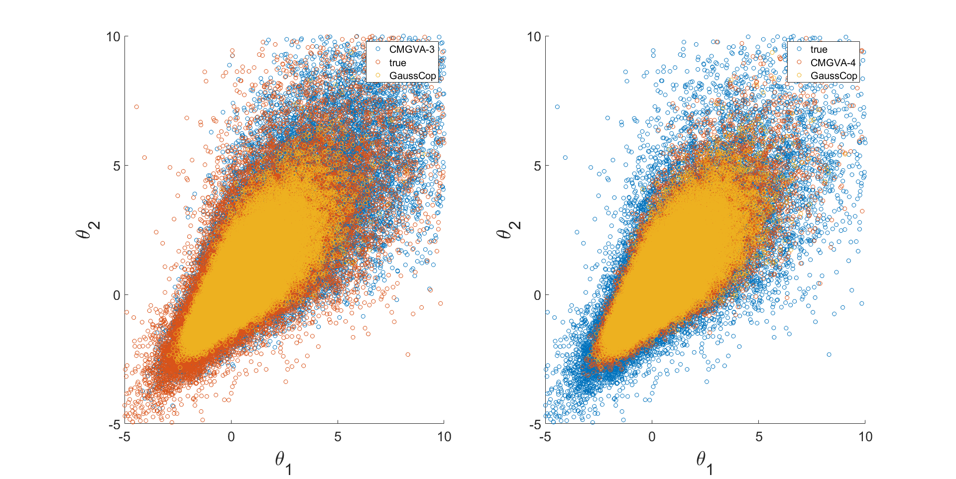
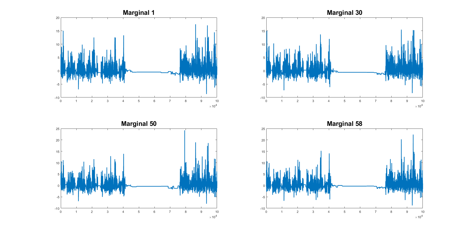
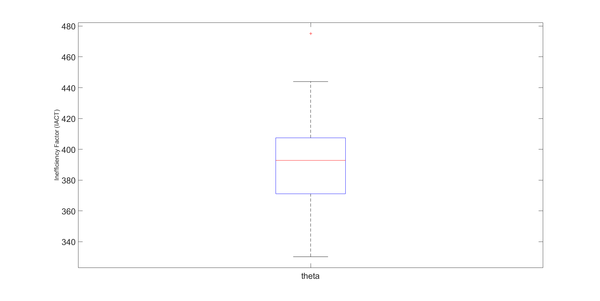
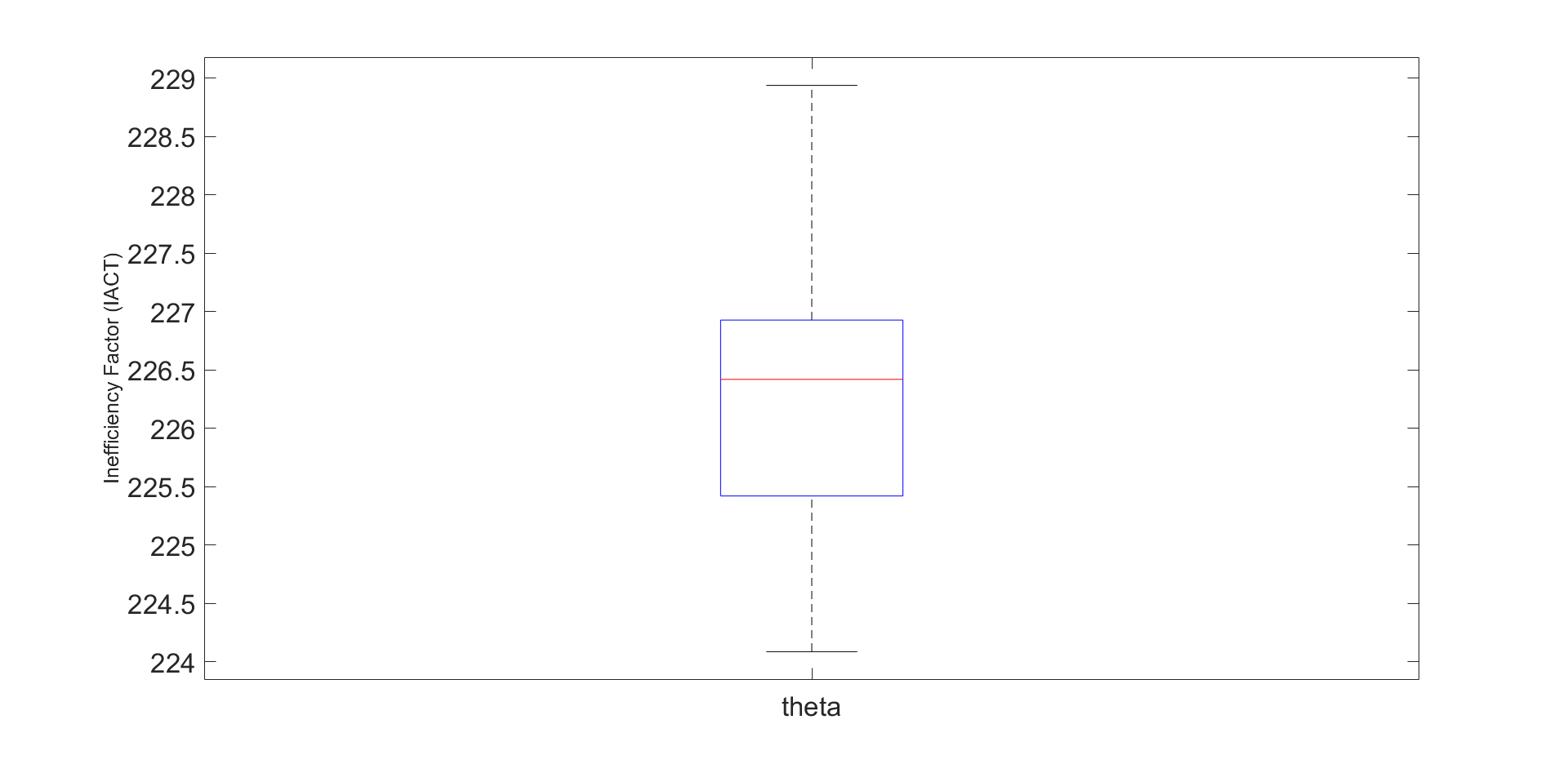
Figure S2 in section S4 of the online supplement shows the IACT of the parameters $\theta$ estimated using the HMC method. The figure shows that the average IACT of the parameters is $391$ with the average effective sample size of $2556.70$ . Figure S1 also shows that the Markov chain sometimes gets stuck, indicating that the HMC method performs quite inefficiently in this example. Figure 4 shows that the 3-component and 4-component CMGVA are more accurate than the HMC method for estimating the marginal density of the parameter $\theta_{1}$ . The same applies to other marginal densities. Again, this suggests that the CMGVA can capture the skewness and heavy-tailed properties of the true target densities.

The CPU time for the HMC method is 167.5 minutes. The time taken for estimating the 3- and 4-component CMGVA are 36.15 minutes and 50.10 minutes³³ 3 The CPU time for estimating the 3-component CMGVA is the total time taken for estimating 1 to 3-component CMGVA. Similar calculations are used for calculating the CPU time for the 4-component CMGVA.. Therefore, the total CPU time for estimating the 3- and 4-component CMGVA are 4.63 and 3.34 times faster than the HMC method.

Refer to caption — Figure 1: Plot of the average lower bound values over the last 500 steps for variational approximations (A1)-(A6) for the 100-dimensional multivariate $t$ -copula example.

5.2 Multimodal High-Dimensional Distributions

This section investigates the ability of the proposed variational approximations (A1)–(A6) to approximate multimodal high-dimensional target distributions. The true target distribution is the multivariate mixture of normals, $\pi\left(\theta\right)=\sum_{c=1}^{3}w_{c}N\left(\theta|u_{c},\Sigma_{c}\right).$ The dimension of the parameters $\theta$ is set to $100$ . Each element $u_{i,c}$ is uniformly drawn from the interval $\left[-2,2\right]$ for $i=1,...,100$ and $c=1,..,3$ . We set the full covariance matrix $\Sigma_{c}$ with ones on the diagonal and the correlation coefficients $\rho=0.2$ and $0.8$ in the off-diagonals for all components. The number of factors $r_{1}=4$ for the first component and $r_{k}=1$ , for each additional mixture component for $k=2,...,20$ for variational approximations A1, A2, A5, and A6. Similarly to the previous example, we use $S=100$ samples to estimate the lower bound values and the gradients of the lower bound. The algorithm in Smith et al., 2020 is performed for $5000$ iterations to obtain the optimal variational parameters for the first component of the mixture and then algorithm 1 is performed for $5000$ iterations to obtain the optimal variational parameters for each additional component of the mixture. The step sizes are set to the values given in section S1 of the online supplement.

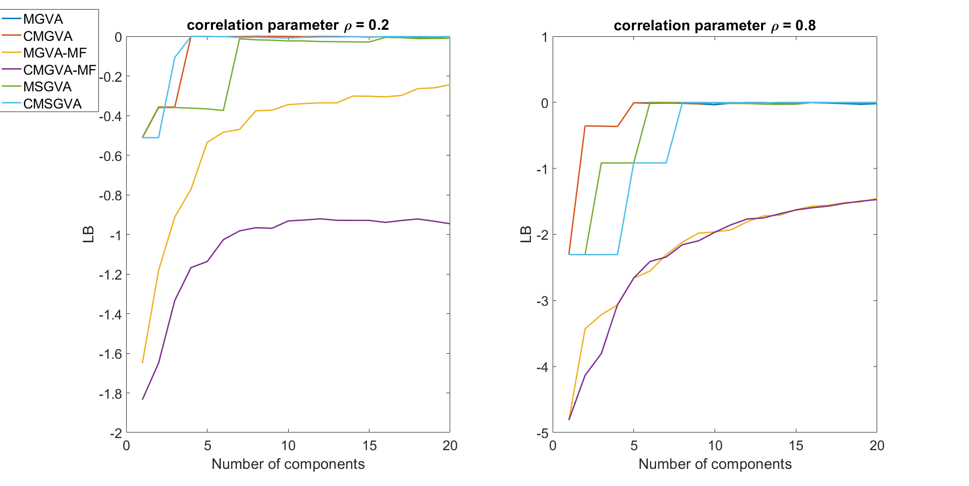
Figure S3 in section S5 of the online supplement shows the average lower bound values over the last 500 steps for the variational approximations (A1)-(A6) for the 100-dimensional mixture of normals example. The figure shows that the performances of the CMGVA, MGVA, MSGVA, and CMSGVA are comparable for the cases $\rho=0.2$ and $\rho=0.8$ . Figure S4 in section S5 of the online supplement confirms that by showing that all the YJ-parameters are close to 1 for CMGVA and CMSGVA and all the $\widetilde{\alpha}$ parameters in Eq. (7) are close to 0 for MSGVA and CMSGVA for the case $\rho=0.8$ . Similar conclusions hold for the case $\rho=0.2$ . The mixture of normals is a special case of CMGVA when all the YJ-parameters are equal to 1, are special cases of MSGVA when all the $\widetilde{\alpha}$ parameters are close to 0, and are special cases of CMSGVA when all the YJ-parameters are close to 1 and all the $\widetilde{\alpha}$ are close to 0. The MGVA, CMGVA, MSGVA, and CMSGVA are clearly much better than MGVA-MF and CMGVA-MF in this example.

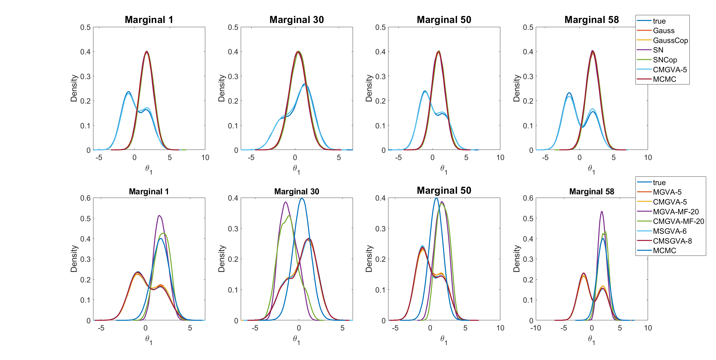
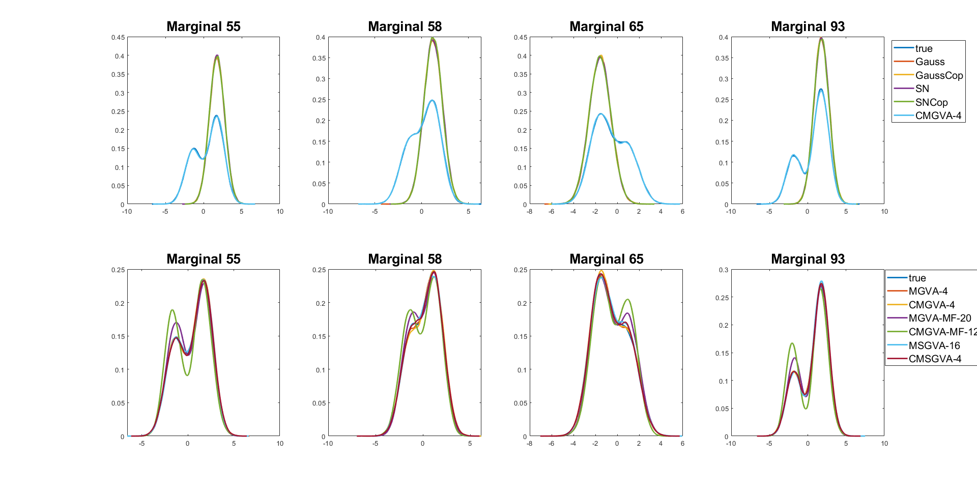
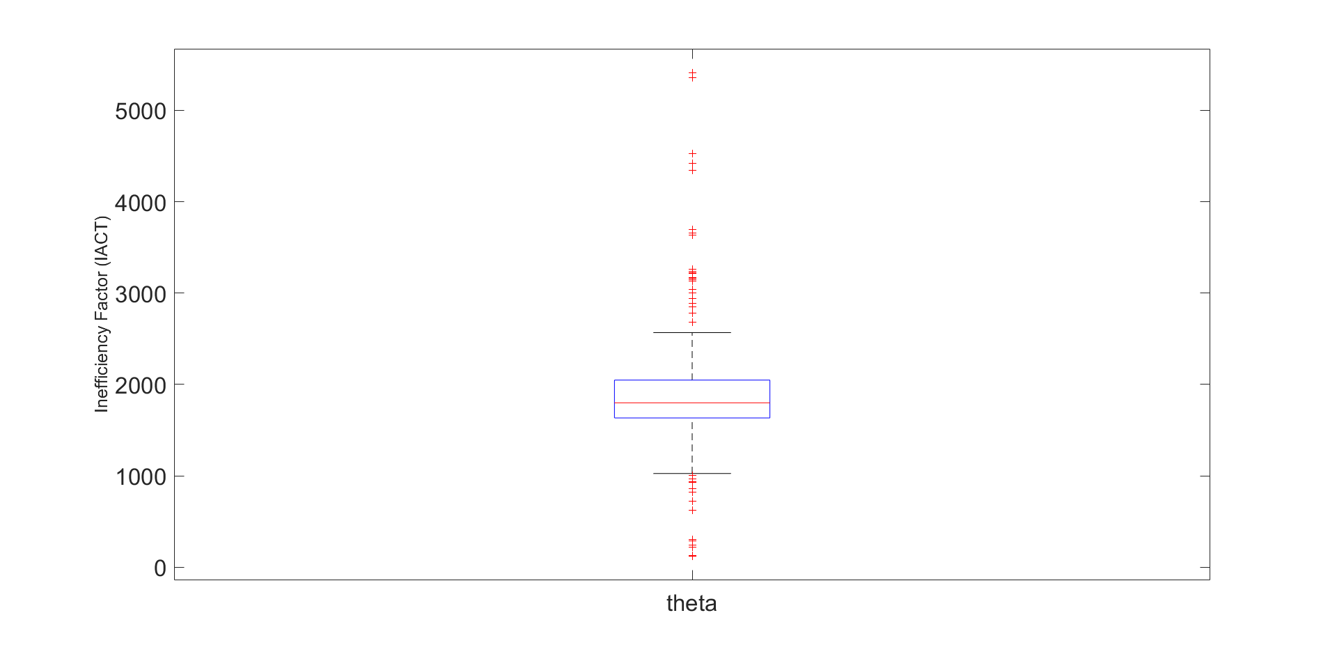
The top panel of figure 5 shows the kernel density estimates of some of the posterior densities of the marginal parameters of $\theta$ approximated with several of the variational approximations, together with the true marginal distributions and the marginal distributions estimated using the HMC method of Hoffman and Gelman, 2014 for the case $\rho=0.8$ . The HMC method ran for $1005000$ iterations, with the initial $5000$ iterations discarded as warm up. The remaining $1000000$ iterations are used for further analysis. Figure S9 in section S5 of the online supplement shows the IACT of the parameters $\theta$ estimated using HMC. The figure shows that the average IACT of the parameters is $226.32$ with the average effective sample size of $4418.52$ , indicating that the HMC method is also quite inefficient for this example.

The bottom panel of figure 5 shows the variational approximations (A1)-(A6), together with the true marginal distributions and the marginal distributions estimated using HMC for $\rho=0.8$ . The top panel shows that the Gaussian, Gaussian copula, skew Gaussian, skew Gaussian copula, and HMC approaches are unable to approximate multimodal distributions. The bottom panel shows that the optimal MGVA, CMGVA, MSGVA, and CMSGVA perform much better than the optimal MGVA-MF and CMGVA-MF. Similar conclusions can be made from figure S5 in section S5 of the online supplement for the case $\rho=0.2$ . The CPU time for the HMC method for this example is $83.75$ minutes. The time taken to estimate the 5-component CMGVA is 37.25 minutes which is $2$ and a quarter times faster than HMC.

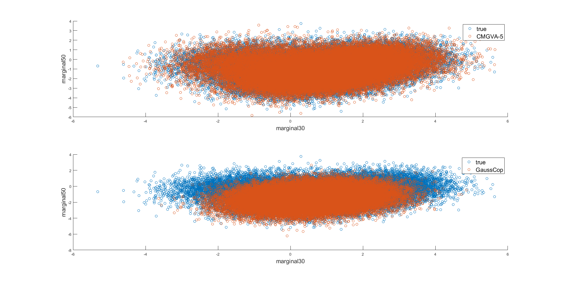
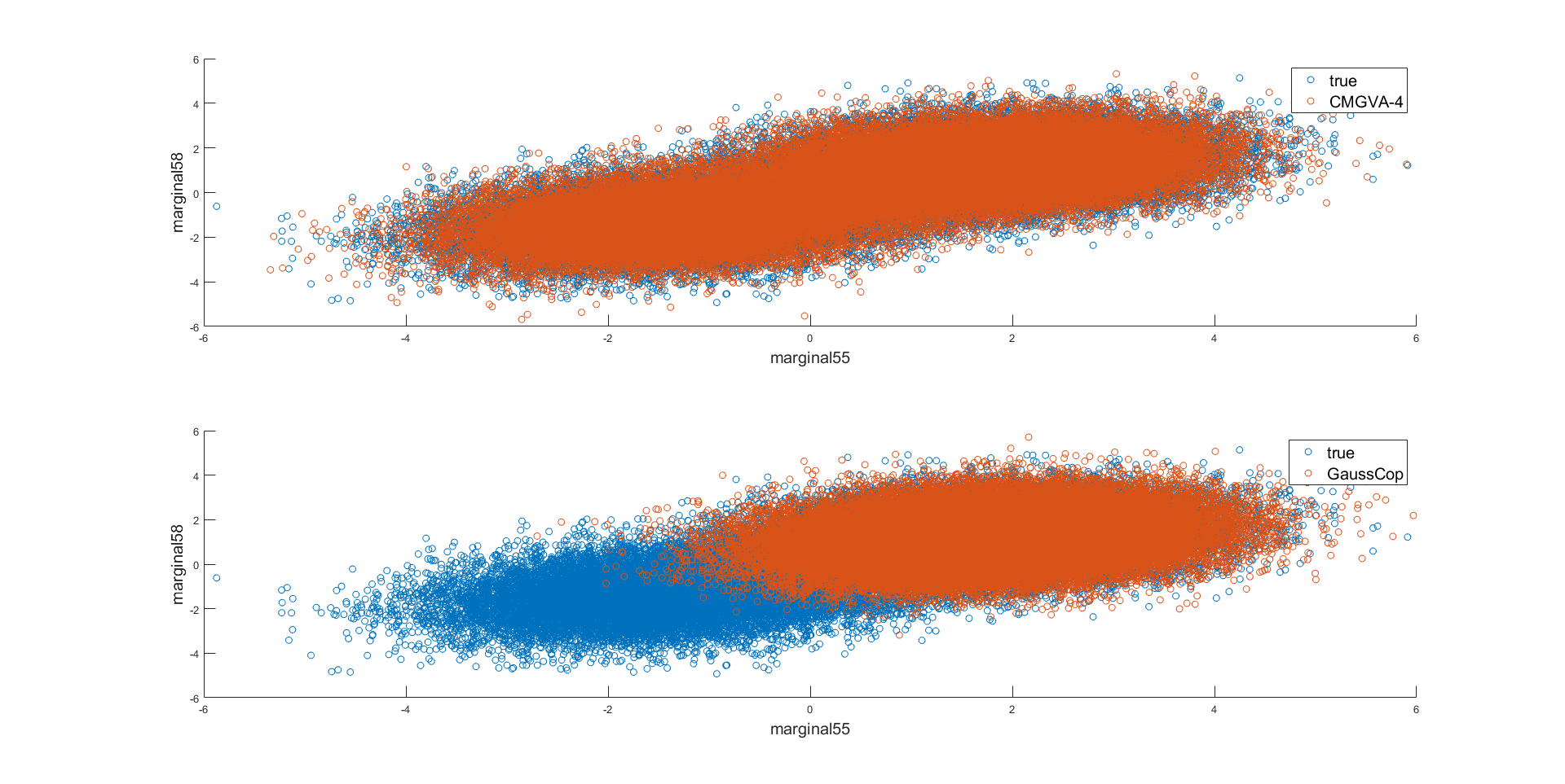
Finally, figures 6 and S6 in section S5 of the online supplement show the scatter plots of the observations generated from the true density, the Gaussian copula variational approximation, and the optimal CMGVA for $\rho=0.8$ and $0.2$ , respectively. The figures confirm that the CMGVA can capture the bimodality and complex-shaped of the two dimensional distribution of the parameters.

We now show that the CMGVA does not overfit a Gaussian target distribution, which we take as a $q$ -variate normal with zero mean and full covariance matrix with ones on the diagonal and correlation coefficients $\rho=0.8$ in the off-diagonals. Figure S7 in section S5 of the online supplement plots the average lower bound values over the last 500 steps for the CMGVA for this example and shows that no improvement is obtained by adding additional components in the mixture.

The two examples in sections 5.1 and 5.2 suggest that: (1) The CMGVA can approximate heavy tails, multimodality, skewness and other complex properties of the high dimensional target distributions, outperforming the Gaussian copula and other variational approximations. Section 5.1 shows that the Gaussian copula outperforms MGVA, MGVA-MF, CMGVA-MF, MSGVA, and CMSGVA at approximating a skewed target distribution. The optimal variational approximations (A1)-(A6) are better than a Gaussian copula at approximating multimodal target distributions. (2) Adding a few components to the MGVA, CMGVA, MSGVA, and CMSGVA generally improves their ability to approximate complex target distributions. Therefore, the proposed approach can be considered as a refinement of the Gaussian copula and skew Gaussian copula variational approximations. (3) Adding additional components one at a time provides a practical method for constructing an increasingly complicated approximation and applies to a variety of multivariate target distributions. (4) The HMC method of Hoffman and Gelman, 2014 fails to estimate the high dimensional, heavy tailed, and multimodal target distribution.

5.3 Bayesian Logistic Regression Models with Complex Prior Distributions

This section considers a logistic regression model

p\left(y_{i}|x_{i},b\right)=\frac{\exp\left(y_{i}x_{i}^{\top}b\right)}{1+\exp\left(y_{i}x_{i}^{\top}b\right)},

with the response $y_{i}\in\left\{0,1\right\}$ , and with a complex prior distribution for the regression parameters $b=(b_{0},b_{1},...,b_{p})^{\top}$ . The prior for each regression parameter, except the intercept, is the two-component mixture of skew normals

p\left(b_{i}|w,\sigma_{1}^{2},\sigma_{2}^{2},\alpha\right)=wSN\left(b_{i};0,\sigma_{1}^{2},\alpha\right)+\left(1-w\right)SN\left(b_{i};0,\sigma_{2}^{2},\alpha\right),\;i=1,...,p;

(16)

$SN\left(b_{i};0,\sigma^{2},\alpha\right)$ is the skew-normal distribution of Azzalini, 1985 with density $\frac{2}{\sigma}\phi\left(\frac{b_{i}}{\sigma}\right)\Phi\left(\alpha\frac{b_{i}}{\sigma}\right)$ . We set $w=0.5$ , $\sigma_{1}^{2}=0.01$ , $\sigma_{2}^{2}=100$ , and $\alpha=-4$ . This prior is motivated by a variable selection scenario, where some coefficients may be 0 and we would like to set these close to zero. The prior for the intercept term $b_{0}$ is $N(0,1)$

We consider the spam, krkp, ionosphere, and mushroom data for the logistic regression model; they have sample sizes $n=4601$ , $351$ , $3196$ , and $8124$ , with $104$ , $111$ , $37$ , and $95$ covariates, respectively and are also considered by Ong et al., 2018 and Smith et al., 2020; the data are available from the UCI Machine Learning Repository (Lichman, 2013)⁴⁴ 4 see https://archive.ics.uci.edu/ml/datasets.php for further details.. In the results reported below, we include all covariates but only use the first $50$ observations of each dataset. The small dataset size and the complex prior distribution for each regression parameter are chosen to create a complex posterior structure to evaluate the performance of variational approximations (A1)-(A6) when the posteriors are non-Gaussian.

Similarly to the previous example, we set the number of factors $r_{1}$ to $4$ for the first component and $r_{k}=1$ , for each additional mixture component for $k=2,...,20$ for variational approximations A1, A2, A5, and A6. We use $S=100$ samples to estimate the lower bound values and the gradients of the lower bound. The algorithm in Smith et al., 2020 is performed for 5000 iterations to obtain the optimal variational parameters for the first component of the mixture and then algorithm 1 is performed for 5000 iterations to obtain the optimal variational parameters for each additional component of the mixture.

Figure 7 shows the average lower bound values over the last 500 steps of the optimisation algorithm for the variational approximations (A1)-(A6) for the Bayesian logistic regression model for the four datasets. The Gaussian and skew Gaussian copula variational approximations outperform the Gaussian and skew Gaussian variational approximations. Interestingly, the mean-field Gaussian copula variational approximation is better than the skew Gaussian and the Gaussian variational approximation for the spam, mushroom, and ionosphere datasets. The figure also shows that adding a few components in the mixture for variational approximations (A1)-(A6) improves the lower bound values for all datasets. The optimal CMGVA performs the best for the spam and krkp datasets. The CMSGVA performs slightly better than CMGVA for the mushroom and ionosphere datasets.

5.4 Flexible Bayesian Regression with a Deep Neural Network

Deep feedforward neural network (DFNN) models with binary and continuous response variables are widely used for classification and regression in the machine learning literature. The DFNN method can be viewed as a way to efficiently transform a vector of $p$ raw covariates $X=\left(X_{1},...,X_{p}\right)^{\top}$ into a new vector $Z$ having the form

Z:=f_{L}\left(W_{L,}f_{L-1}\left(W_{L-1},...,f_{1}\left(W_{1},X\right)\right)\right).

(17)

Each $Z_{l}=f_{l}\left(W_{l},Z_{l-1}\right)$ , $l=1,...,L$ , is called a hidden layer, $L$ is the number of hidden layers in the network, $W=\left(W_{1},...,W_{L}\right)$ is the set of weights and $Z_{0}=X$ by construction. The function $f_{l}\left(W_{l},Z_{l-1}\right)$ is assumed to be of the form $h_{l}\left(W_{l}Z_{l-1}\right)$ , where $W_{l}$ is a matrix of weights that connect layer $l-1$ to layer $l$ , which includes weight coefficients attached to the input $Z_{l-1}$ and the constant terms, and $h_{l}\left(\cdot\right)$ is a scalar activation function. Estimation in complex high dimensional models like DFNN regression models is challenging. This section studies the accuracy of posterior densities and the predictive performance of the variational approximations (A1)-(A6) for a DFNN regression model with continuous responses; see Goodfellow et al., 2016 for a comprehensive recent discussion of DFNNs and other types of neural networks.

Consider a dataset $D$ with $n$ observations, with $y_{i}$ the scalar response and $x_{i}=\left(x_{i1},...,x_{ip}\right)^{\top}$ the vector of $p$ covariates. We consider a neural network structure with the input vector $x$ and a scalar output. Denote $z_{l}:=f_{l}\left(x,w\right)$ , $l=1,...,M$ , the units in the last hidden layer, $w$ is the vector of weights up to the last hidden layer, and $b=\left(b_{0},b_{1},...,b_{M}\right)^{\top}$ are the weights that connect the variable $z_{l}$ , $l=1,...,M$ , to the output $y$ . The model, with a continuous response $y$ , can be written as

$\displaystyle\tau^{2}$	$\displaystyle\sim$	$\displaystyle Gamma\left(1,10\right),$	(18)
$\displaystyle w_{i}$	$\displaystyle\sim$	$\displaystyle 0.5SN\left(0,\sigma_{1}^{2},\alpha\right)+0.5SN\left(0,\sigma_{2}^{2},\alpha\right),\;\textrm{for}\;i=1,...,M_{w},$	(19)
$\displaystyle b_{l}$	$\displaystyle\sim$	$\displaystyle 0.5SN\left(0,\sigma_{1}^{2},\alpha\right)+0.5SN\left(0,\sigma_{2}^{2},\alpha\right),\;\textrm{for}\;l=1,...,M,$	(20)
$\displaystyle y\|x,w,b,\tau$	$\displaystyle\sim$	$\displaystyle N\left(b_{0}+\widetilde{b}^{\top}z,1/\tau^{2}\right),$	(21)

where $z=(z_{1},...,z_{M})^{\top}$ , $\widetilde{b}=(b_{1},...,b_{M})^{\top}$ , $M_{w}$ is the number of weight parameters; $SN\left(B;0,\sigma^{2},\alpha\right)$ is a skew-normal density of Azzalini, 1985 defined in Section 5.3, and $Gamma\left(1,10\right)$ is the gamma distribution with shape parameter 1 and scale parameter 10. We set $\sigma_{1}^{2}=0.01$ , $\sigma_{2}^{2}=100$ , and $\alpha=-4$ . Miller et al., 2017 uses similar priors for $\tau^{2}$ . The priors for $b_{l}$ for $l=1,...,M$ and $w_{i}$ for $i=1,...,M_{w}$ will shrink some of the coefficients that may be 0 or very close to zero.

All the examples use the rectified linear unit (ReLU) $h\left(x\right):=\max\left(0,x\right)$ as an activation function, unless otherwise stated; ReLU is widely applied in the deep learning literature (Goodfellow et al., 2016) because it is easy to use within optimization as it is quite similar to a linear function, except that it outputs zero for negative values of $x$ .

We consider the auto and abalone datasets. The auto dataset, available from James et al., 2021, consists of 392 observations for different makes of cars, with the response being gas mileage in miles per gallon, with 7 additional covariates used here to predict the mileage. The abalone dataset, available on the UCI Machine Learning Repository, has 4177 observations. The response variable is the number of rings used to determine the age of the abalone. There are 9 covariates including sex, length, diameter, as well as other measurements of the abalone. We use 90% of the data for training and the rest for computing the log of the approximate predictive score in Eq. (24). Both datasets have continuous responses

Neural nets with (8,5,5,1), (8,10,10,1) and (8,20,20,1) structures are used for the auto dataset. For the (8,5,5,1) structure, the input layer has 8 variables, there are two hidden layers each having 5 units and there is a scalar output. The first layer has $8\times 5=40$ $w$ parameters, the second layer has $6\times 5=30$ $w$ parameters (including the intercept term), and $6$ $b$ parameters (including the intercept term); this gives a total of $76$ parameters. Similar calculations can be made for the (8,10,10,1) and (8,20,20,1) structures to give a total of $201$ and $601$ parameters, respectively. Neural nets with (9,5,5,1), (9,10,10,1) and (9,20,20,1) structures are used for the abalone data set. Similar calculations can be done for them to give a total of $75$ , $211$ , and $621$ parameters, respectively.

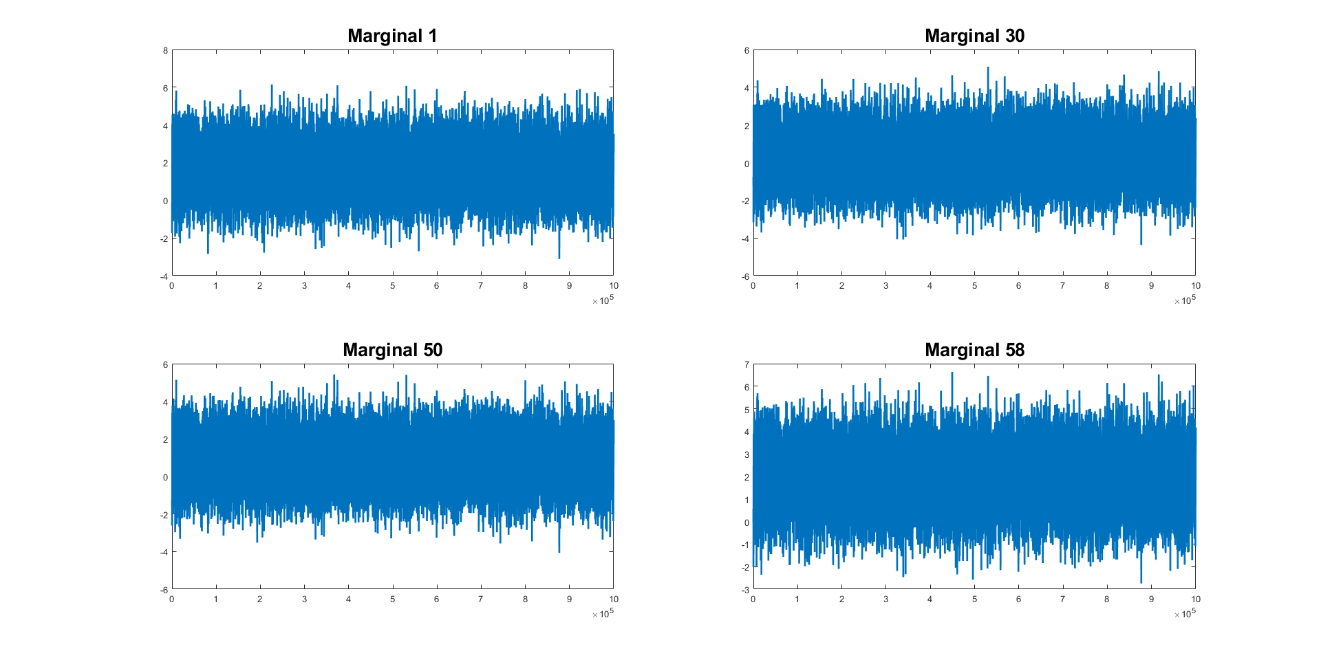
This section studies the accuracy of the inference and the predictive performance for variational approximations A1 and A2. For this example, variational approximations A5 and A6 are not implemented due to the numerical issues in estimating the skew normal and skew normal copula variational approximations. Sections 5.1 to 5.3 show that CMGVA is better than MSGVA and CMSGVA. We do not compare the posterior density of the parameters obtained from the variational approximations A1 and A2 to HMC, as it is difficult to obtain the exact posterior distribution for the parameters of the Bayesian neural network. Papamarkou et al., 2021 shows that the Markov chains generated by the Metropolis-Hastings and Hamiltonian Monte Carlo methods fail to converge for estimating the parameters of the Bayesian neural network model. To show the lack of convergence of the HMC method, we ran it for $1005000$ iterations discarding the initial $5000$ iterations as warm up for estimating neural nets with a (9,10,10,1) structure for the auto dataset. Figure S14 in section S8 of the online supplement shows the IACT of the parameters $\theta$ estimated using the HMC method. The figure shows that the average IACT of the parameters is $1904.08$ with an average effective sample size of $525.19$ , indicating that HMC is very inefficient for this example. In addition, figure S13 in section S8 of the online supplement shows the trace plots of the parameters of the neural net with the (9,10,10,1) structure for the auto dataset. The figure shows that the parameters mix poorly. Computing time for a 10-component CMGVA is an order of magnitude less than for the HMC.

To evaluate the predictive accuracy of a DFNN regression model estimated by the variational approximations A1 and A2, we consider the posterior predictive density defined as

p\left(y|x,D\right)=\int p\left(y|x,\theta\right)p\left(\theta|D\right)d\theta.

(22)

Given that we have the variational approximation of the posterior distribution, we can define the approximate predictive density

g\left(y|x,D\right)=\int p\left(y|x,\theta\right)q_{\lambda}\left(\theta\right)d\theta.

(23)

Computing the approximate posterior predictive density in Eq. (23) is challenging because it involves high dimensional integrals that cannot be solved analytically. However, it can be estimated using Monte Carlo integration. The estimate of the log of the approximate posterior predictive score is

\textrm{log}\,\widehat{g}\left(y|x,D\right)=\textrm{log}\left(\frac{1}{R}\sum_{r=1}^{R}p\left(y|x,\theta^{r}\right)\right),\;\theta^{r}\sim q_{\lambda}\left(\theta\right).

(24)

The higher the log of the approximate posterior predictive score, the more accurate the prediction.

In this example, the number of factors is set to 1 for all $20$ components in the mixture; $S=200$ samples are used to estimate the gradients of the lower bound; $R=10000$ samples are used to estimate the log of the approximate posterior predictive score in Eq. (24); section S7 of the online supplement discusses the stopping criterion for the optimisation algorithm.

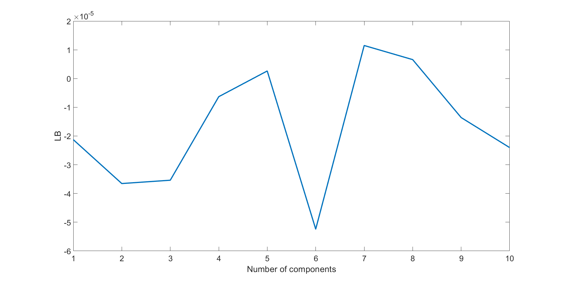
The top panels of figure S15 in section S8 of the online supplement show the average lower bound values over the last 100 steps of the optimisation algorithm for the (8,5,5,1) neural net structure for the auto dataset and the (9,5,5,1) structure for the abalone dataset. The figure shows that adding components to the variational approximations A1 and A2 increases the lower bound significantly for both datasets. Clearly, CMGVA performs best for both datasets. The lower panels of figure S15 show the log of the estimated approximate posterior predictive scores evaluated for the test data. The figure also shows that adding more components to the variational approximations can improve the prediction accuracy significantly. Similar conclusions can be drawn from figure 8 for the (8,10,10,1) neural net structure for the auto dataset and the (9,10,10,1) neural net structure for the abalone dataset and figure 9 for the (8,20,20,1) neural net structure for the auto dataset and the (9,20,20,1) neural net structure for the abalone dataset. This suggests the usefulness of the proposed variational approximations for complex and high-dimensional Bayesian deep neural network regression models.

We now compare the optimal CMGVA to the planar flows of Rezende and Mohamed, 2015 with flow lengths of $10$ transformations. Tanh is the non-linearity function with the initial distribution being Gaussian with mean $\mu$ and a diagonal covariance matrix; $S=1000$ samples are used to accurately estimate the gradients of the lower bound. A similar stopping rule to that described in section S7 of the online supplement is used. Figures S11 and S12 in section S6 of the online supplement show that the lower bound of the planar flows for the two datasets for neural nets with different structures increase at the start and then converge. Table S1 in section S8 of the online supplement shows that the CMGVA has a higher lower bound and higher log of the approximate posterior predictive scores compared to the planar flows.

5.5 Efficiency of the Natural Gradient

This section compares the performance of the natural gradient and the ordinary gradient methods using the same initial values for the variational parameters for both methods. Figure 10 shows the lower bound values over iterations for both methods for the 2-component CMGVA for the multivariate $t$ -copula, multivariate mixture of normals, logistic regression (spam dataset), and Bayesian DFNN regression (abalone dataset with neural net (9, 5, 5, 1) structure). The figure shows that the natural gradient is much less noisy and converges much faster than the ordinary gradient.

6 Conclusion

The article proposes flexible variational approximations based on a copula of a mixture of normals and constructs the computational algorithms for estimating the approximation. An important part of the approach is the construction of appropriate transformations of the parameters to try and simplify the joint posterior which is then estimated by a mixture of normals.

The VB method is made efficient by using the natural gradient and control variates. Our approach of adding one component at a time provides a practical variational inference method that constructs an increasingly complicated posterior approximation and is an extension and refinement of state-of-the-art Gaussian and skew Gaussian copula variational approximations in Smith et al., 2020. The proposed variational approximations apply to a wide range of Bayesian models; we apply it to four complex examples, including Bayesian deep learning regression models, and show that it improves upon the Gaussian copula and mixture of normals variational approximations in terms of both inference and prediction. Our article uses a factor structure for the covariance matrix in our variational approximation, but it is straightforward to extend the variational approach to consider other sparse forms of the covariance structure, such as a sparse Cholesky factorisation as in Tan et al., 2020.

We note that it is straightforward to use any other copula-based approximation as a first component in our approach, such as a $t$ -copula. This may result in a simpler mixture approximation than using the Gaussian copula as a first component.

7 Acknowledgement

The research of Robert Kohn was partially supported by an ARC Center of Excellence grant CE140100049.

8 Online Supplement

CopMixJCGSSupp.pdf (pdf file) provides additional examples, results and technical details. Computer code to implement the methods for the examples of this article is available online.

Online Supplement: Flexible Variational Bayes based on a Copula of a Mixture

S1 Learning Rate

Setting the learning rate in a stochastic gradient algorithm is very challenging, especially when the parameter vector is high dimensional. The choice of learning rate affects both the rate of convergence and the quality of the optimum attained. Learning rates that are too high can cause unstable optimisation, while learning rates that are too low result in slow convergence and can lead to a situation where the parameters erroneously appear to have converged. In all our examples, the learning rates are set adaptively using the ADAM method (Kingma and Ba, 2015) that gives different step sizes for each element of the variational parameters $\lambda$ . At iteration $t+1$ , the variational parameter $\lambda$ is updated as

\lambda^{\left(t+1\right)}:=\lambda^{\left(t\right)}+\triangle^{\left(t\right)}.

Let $g_{t}^{\textrm{nat}}$ denote the natural stochastic gradient estimate at iteration $t$ . ADAM computes (biased) first and second moment estimates of the gradients using exponential moving averages,

	$\displaystyle m_{t}$	$\displaystyle=$	$\displaystyle\tau_{1}m_{t-1}+\left(1-\tau_{1}\right)g_{t}^{\textrm{nat}},$
	$\displaystyle v_{t}$	$\displaystyle=$	$\displaystyle\tau_{2}v_{t-1}+\left(1-\tau_{2}\right)\left(g_{t}^{2}\right)^{\textrm{nat}},$

where $\tau_{1},\tau_{2}\in\left[0,1\right)$ control the decay rates. The biased first and second moment estimates are corrected by (Kingma and Ba, 2015)

\displaystyle\widehat{m}_{t}

\displaystyle=

\displaystyle m_{t}/\left(1-\tau_{1}^{t}\right),\quad\widehat{v}_{t}=v_{t}/\left(1-\tau_{2}^{t}\right);

the change $\triangle^{\left(t\right)}$ is then computed as

\triangle^{\left(t\right)}=\frac{\alpha\widehat{m}_{t}}{\sqrt{\widehat{v}_{t}}+\epsilon}.

We set $\tau_{1}=0.9$ , $\tau_{2}=0.99$ , and $\epsilon=10^{-8}$ (Kingma and Ba, 2015). It is possible to use different $\alpha$ for $\mu$ , $\beta$ , $d$ , and $\pi$ . We set $\alpha_{\mu}=0.01$ , $\alpha_{\beta}=\alpha_{d}=\alpha_{\pi}=0.001$ , unless stated otherwise.

S2 Algorithms

Algorithm S1 gives the formula for computing the natural gradients for the vectors $\beta_{K+1}$ and $d_{K+1}$ .

Algorithm S1 Computing the natural gradients for the vectors

\beta_{K+1}

and

d_{K+1}

Input: vectors $\beta_{K+1}$ and $d_{K+1}$ and the standard gradients $g_{\beta_{K+1}}=\nabla_{\textrm{vech}\left(\beta_{K+1}\right)}\mathcal{L}\left(\lambda\right)$ and $g_{d_{K+1}}=\nabla_{d_{K+1}}\mathcal{L}\left(\lambda\right)$

Output: $g_{\beta_{K+1}}^{\textrm{nat}}=F_{\lambda}^{-1}g_{\beta_{K+1}}=\nabla_{\textrm{vech}\left(\beta_{K+1}\right)}^{\textrm{nat}}\mathcal{L}\left(\lambda\right)$ and $g_{d_{K+1}}^{\textrm{nat}}=F_{\lambda}^{-1}g_{d_{K+1}}=\nabla_{d_{K+1}}^{\textrm{nat}}\mathcal{L}\left(\lambda\right)$ .

•

Compute the vectors: $v_{1}=d_{K+1}^{2}-2\beta_{K+1}^{2}\circ d_{K+1}^{-4}$ , $v_{2}=\beta_{K+1}^{2}\circ d_{K+1}^{-3}$ , and the scalars $\kappa_{1}=\sum_{i=1}^{m}\beta_{K+1}^{2}/d_{K+1}^{2}$ , and $\kappa_{2}=0.5\left(1+\sum_{i=1}^{m}v_{2i}^{2}/v_{1i}\right)^{-1}$ .

•

Compute:

g_{\beta_{K+1}}^{\textrm{nat}}=\frac{1+\kappa_{1}}{2\kappa_{1}}\left(\left(g_{\beta_{K+1}}^{\top}\beta_{K+1}\right)\beta_{K+1}+d_{K+1}^{2}\circ g_{\beta_{K+1}}\right),

(S1)

and

g_{d_{K+1}}^{\textrm{nat}}=0.5v_{1}^{-1}\circ g_{d_{K+1}}+\kappa_{2}\left[\left(v_{1}^{-1}\circ v_{2}\right)^{\top}g_{d_{K+1}}\right]\left(v_{1}^{-1}\circ v_{2}\right).

(S2)

S3 Integrated Autocorrelation Time

To define our measure of the inefficiency of an MCMC sampler, we define the integrated autocorrelation time (IACT) for a univariate function $\psi(\theta)$ of parameter $\theta$ as

\textrm{IACT}_{\psi}=1+2\sum_{j=1}^{\infty}\rho_{j,\psi},

where $\rho_{j,\psi}$ is the $j$ th autocorrelation of the iterates of $\psi(\theta)$ in the MCMC after the chain has converged. It measures the inefficiency of the sampling scheme in terms of the multiple of its draws that are required to obtain the same variance as an independent sampling scheme, e.g. if IACT = 10, then we need ten times as many iterates as an independent scheme. We use the CODA package of Plummer et al., 2006 to estimate the IACT values of the parameters. A low value of the IACT estimate suggests that the Markov chain mixes well.

S4 Additional Figures for the Skewed and Heavy-Tailed High-Dimensional Target Distribution Example

S5 Additional Figures for the Multimodal High-Dimensional Target Distribution Example

This section gives additional figures for the multimodal high-dimensional target distribution example in section 5.2.

S6 Planar Flows

This section discusses variational inference using planar flows proposed by Rezende and Mohamed, 2015. The planar flows consider a family of transformations of the form

f\left(\theta\right)=\theta+uh\left(w^{\top}\theta+b\right),

where $\lambda=\left\{w\in R^{D},u\in R^{D},b\in R\right\}$ are the variational parameters and $h\left(\cdot\right)$ is a smooth elementwise non-linearity with derivative $h^{{}^{\prime}}\left(\cdot\right)$ . The log determinant of the Jacobian term is

\log\left|\det\frac{\partial f\left(\theta\right)}{\partial\theta}\right|=\log\left|1+u^{\top}\psi\left(\theta\right)\right|,

(S3)

where $\psi\left(\theta\right)=h^{{}^{\prime}}\left(w^{\top}\theta+b\right)w$ . The density of $q_{K}\left(\theta\right)$ is obtained by successively transforming a random variable $\theta_{0}$ with distribution $q_{0}$ through a chain of $K$ transformations is

	$\displaystyle\theta_{K}$	$\displaystyle=$	$\displaystyle f_{K}\circ...\circ f_{2}\circ f_{1}\left(\theta_{0}\right),$		(S4)
	$\displaystyle\log q_{K}\left(\theta_{K}\right)$	$\displaystyle=$	$\displaystyle\log q_{0}\left(\theta_{0}\right)-\sum_{k=1}^{K}\log\left\|1+u_{k}^{\top}\psi_{k}\left(\theta_{k-1}\right)\right\|.$		(S5)

Section 5.4 compares the proposed variational approximations with the planar flows with flow lengths of $10$ transformations for the neural nets with (8,5,5,1), (8,10,10,1), and (8,20,20,1) structures for the auto dataset and neural nets with (9,5,5,1), (9,10,10,1), and (9,20,20,1) structures for the abalone dataset. The non-linearity function $h\left(\cdot\right)$ is the tanh function and the initial distribution is a Gaussian distribution with a mean vector $\mu$ and a diagonal covariance matrix with elements $d=\left(d_{1},...,d_{M}\right)$ , where $M$ is the number of parameters. We use $S=1000$ samples to accurately estimate the gradients of the lower bound. The optimisation algorithm is stopped if it exceeds $10000$ iterations or the lower bound does not improve after $20$ iterations. To reduce the noise in estimating the lower bound, we take the average of the lower bound over a moving window of $250$ iterations (see Tran et al., 2017, for further details). We also use the momentum method (Polyak, 1964) to help accelerating stochastic gradient optimisation and reduce the noise in the estimated gradients of the lower bound.

Figures S11 and S12 show that the lower bound of the planar flows for the two datasets for neural nets with different structures increase at the start and then converge.

S7 Stopping Criterion for the Flexible Bayesian Regression with a Deep Neural Network Example

This section discusses the stopping criterion used for the optimisation algorithm in Section 5.4. The algorithm is stopped if it exceeds $P$ iterations or the lower bound does not improve after $20$ iterations. For the first component, we set $P$ to $5000$ iterations and for the subsequent components, we set $P$ to $1000$ iterations, with the exception of the neural nets (8,20,20,1) for the auto dataset and (9,20,20,1) for the abalone dataset, where we set $P$ to $5000$ due to a greater number of parameters. To reduce the noise in estimating the lower bound, we average the lower bound over a moving window of $100$ iterations for the first component and $250$ for the additional components due to more challenging optimisation problems (see Tran et al., 2017, for further details). We also use the momentum method (Polyak, 1964) to help accelerating stochastic gradient optimisation and reduce the noise in the estimated gradients of the lower bound for the first component. The step sizes are set to the values given in section S1 of the online supplement, except $\alpha_{\mu}$ is set to 0.001.

S8 Additional Figures and Tables for the Flexible Bayesian Regression with a Deep Neural Network Example

Figure S13 shows the trace plots of the parameters of the neural net with the (9,10,10,1) structure for the auto dataset. The parameters do not show evidence of convergence even after $1000000$ iterations.

Table S1: Comparing the performance of optimal variational approximation A2 (with the number in bracket indicating the optimal number of components) with the planar flow with flow lengths of

10

transformations in terms of lower bound (top panel) and predictive values (bottom panel).

Data	Neural Nets	Planar	Optimal A2
Abalone	$\left(9,5,5,1\right)$	$-8495.38$	$-8322.75(10)$
	$\left(9,10,10,1\right)$	$-8657.56$	$-8492.98(10)$
	$\left(9,20,20,1\right)$	$-9481.93$	$-8786.62(10)$
Auto	$\left(8,5,5,1\right)$	$-1127.39$	$-996.41(10)$
	$\left(8,10,10,1\right)$	$-1255.76$	$-1092.79(10)$
	$\left(8,20,20,1\right)$	$-1560.68$	$-1389.68(10)$
Abalone	$\left(9,5,5,1\right)$	$-914.80$	$-904.60(6)$
	$\left(9,10,10,1\right)$	$-912.97$	$-893.18(10)$
	$\left(9,20,20,1\right)$	$-920.56$	$-906.51(6)$
Auto	$\left(8,5,5,1\right)$	$-98.05$	$-95.06(10)$
	$\left(8,10,10,1\right)$	$-98.09$	$-95.19(9)$
	$\left(8,20,20,1\right)$	$-98.08$	$-95.30(8)$

References

Amari, (1998) Amari, S. (1998). Natural gradient works efficiently in learning. Neural Computation, 10(2):251–276.
Azzalini, (1985) Azzalini, A. (1985). A class of distributions which includes the normal ones. Scandinavian Journal of Statistics, 12(2):171–178.
Blei et al., (2017) Blei, D. M., Kucukelbir, A., and McAuliffe, J. D. (2017). Variational inference: a review for statisticians. Journal of American Statistical Association, 112(518):859–877.
Bottou, (2010) Bottou, L. (2010). Large-scale machine learning with stochastic gradient descent. In Proceedings of the 19th International Conference on Computational Statistics (COMPSTAT2010), pages 177–187. Springer.
Campbell and Li, (2019) Campbell, T. and Li, X. (2019). Universal boosting variational inference. Advances in Neural Information Processing Systems, 32.
Challis and Barber, (2013) Challis, E. and Barber, D. (2013). Gaussian Kullback-Leibler approximate inference. Journal of Machine Learning Research, 14:2239–2286.
Goodfellow et al., (2016) Goodfellow, I., Bengio, Y., and Courville, A. (2016). Deep Learning. MIT Press.
Guo et al., (2017) Guo, F., Wang, X., Broderick, T., and Dunson, D. B. (2017). Boosting variational inference. ArXiv: 1611.05559v2.
Hoffman et al., (2013) Hoffman, M. D., Blei, D. M., Wang, C., and Paisley, J. (2013). Stochastic variational inference. Journal of Machine Learning Research, 14:1303–1347.
Hoffman and Gelman, (2014) Hoffman, M. D. and Gelman, A. (2014). The no-u-turn sampler: adaptively setting path lengths in Hamiltonian Monte Carlo. Journal of Machine Learning Research, 15(1):1593–1623.
Izmailov et al., (2021) Izmailov, P., Vikram, S., Hoffman, M. D., and Wilson, A. G. (2021). What are Bayesian neural network posteriors really like? In International Conference on Machine Learning, pages 4629–4640. PMLR.
James et al., (2021) James, G., Witten, D., Hastie, T., and Tibshirani, R. (2021). An introduction to statistical learning: with applications in R. New York, Springer, 2nd Edition.
Jerfel et al., (2021) Jerfel, G., Wang, S. L., Fannjiang, C., Heller, K. A., Ma, Y., and Jordan, M. (2021). Variational refinement for importance sampling using the forward Kullback-Leibler divergence. In de Campos, C. and Maathuis, M., editors, Uncertainty in Artificial Intelligence (UAI), Proceedings of the Thirty-Seventh Conference.
Jospin et al., (2022) Jospin, L. V., Laga, H., Boussaid, F., Buntine, W., and Bennamoun, M. (2022). Hands-on Bayesian neural networks – A tutorial for deep learning users. IEEE Computational Intelligence Magazine, 17(2):29–48.
Khaled and Kohn, (2023) Khaled, M. and Kohn, R. (2023). On approximating copulas by finite mixtures. https://arxiv.org/pdf/1705.10440.pdf.
Khan and Lin, (2017) Khan, M. E. and Lin, W. (2017). Conjugate-computation variational inference: Converting variational inference in non-conjugate models to inferences in conjugate models. In Singh, A. and Zhu, X. J., editors, Proceedings of the 20th International Conference on Artificial Intelligence and Statistics, AISTATS 2017, 20-22 April 2017, Fort Lauderdale, FL, USA, volume 54, pages 878–887. PMLR.
Khan and Nielsen, (2018) Khan, M. E. and Nielsen, D. (2018). Fast yet simple natural-gradient descent for variational inference in complex models. In International Symposium on Information Theory and Its Applications, ISITA 2018, Singapore, October 28-31, 2018, pages 31–35. IEEE.
Kingma and Ba, (2015) Kingma, D. P. and Ba, J. (2015). Adam: A method for stochastic optimization. In Bengio, Y. and LeCun, Y., editors, 3rd International Conference on Learning Representations, ICLR 2015, San Diego, CA, USA, May 7-9, 2015, Conference Track Proceedings.
Kingma and Welling, (2014) Kingma, D. P. and Welling, M. (2014). Auto-encoding variational Bayes. In 2nd International Conference on Learning Representations, ICLR 2014, Banff, AB, Canada, April 14-16, 2014, Conference Track Proceedings.
Kleijnen and Rubinstein, (1996) Kleijnen, J. P. C. and Rubinstein, R. Y. (1996). Optimisation and sensitivity analysis of computer simulation models by the score function method. European Journal of Operational Research, 88(3):413–427.
Kucukelbir et al., (2017) Kucukelbir, A., Tran, D., Ranganath, R., Gelman, A., and Blei, D. M. (2017). Automatic differentiation variational inference. Journal of machine learning research, 18(14):1–45.
Lichman, (2013) Lichman, M. (2013). UCI machine learning repository. University of California, Irvine, School of Information and Computer Sciences.
Lin et al., (2019) Lin, W., Khan, M. E., and Schmidt, M. (2019). Fast and simple natural-gradient variational inference with mixture of exponential-family approximations. In Chaudhuri, K. and Salakhutdinov, R., editors, Proceedings of the 36th International Conference on Machine Learning, volume 97 of Proceedings of Machine Learning Research, pages 3992–4002. PMLR.
Locatello et al., (2018) Locatello, F., Khanna, R., Ghosh, J., and Ratsch, G. (2018). Boosting variational inference: an optimization perspective. In Storkey, A. and Perez-Cruz, F., editors, Proceedings of the Twenty-First International Conference on Artificial Intelligence and Statistics, volume 84 of Proceedings of Machine Learning Research, pages 464–472. PMLR.
Miller et al., (2017) Miller, A. C., Foti, N. J., and Adams, R. P. (2017). Variational boosting: Iteratively refining posterior approximations. In Precup, D. and Teh, Y. W., editors, Proceedings of the 34th International Conference on Machine Learning, volume 70 of Proceedings of Machine Learning Research, pages 2420–2429. PMLR.
Nott et al., (2012) Nott, D. J., Tan, S., Villani, M., and Kohn, R. (2012). Regression density estimation with variational methods and stochastic approximation. Journal of Computational and Graphical Statistics, 21:797–820.
Ong et al., (2018) Ong, M. H. V., Nott, D. J., and Smith, M. S. (2018). Gaussian variational approximation with a factor covariance structure. Journal of Computational and Graphical Statistics, 27(3):465–478.
Ormerod and Wand, (2010) Ormerod, J. T. and Wand, M. P. (2010). Explaining variational approximations. American Statistician, 64:140–153.
Paisley et al., (2012) Paisley, J., Blei, D. M., and Jordan, M. I. (2012). Variational Bayesian inference with stochastic search. In Proceedings of the 29th International Conference on Machine Learning, ICML’12, pages 1363–1370, Madison, WI, USA. Omnipress.
Papamakarios et al., (2021) Papamakarios, G., Nalisnick, E., Rezende, D. J., Mohamed, S., and Lakshminarayanan, B. (2021). Normalizing flows for probabilistic modeling and inference. The Journal of Machine Learning Research, 22(1):2617–2680.
Papamarkou et al., (2021) Papamarkou, T., Hinkle, J., Young, M., and Womble, D. (2021). Challenges in Markov chain Monte Carlo for Bayesian neural networks. arXiv:1910.06539v6.
Plummer et al., (2006) Plummer, M., Best, N., Cowles, K., and Vines, K. (2006). CODA: Convergence Diagnosis and Output Analysis of MCMC. R News, 6(1):7–11.
Polyak, (1964) Polyak, B. T. (1964). Some methods of speeding up the convergence of iteration methods. USSR computational mathematics and mathematical physics, 4(5):1–17.
Ranganath et al., (2014) Ranganath, R., Gerrish, S., and Blei, D. M. (2014). Black box variational inference. In Kaski, S. and Corander, J., editors, Proceedings of the Seventeenth International Conference on Artificial Intelligence and Statistics, volume 33 of Proceedings of Machine Learning Research, pages 814–822, Reykjavik, Iceland. PMLR.
Rezende and Mohamed, (2015) Rezende, D. and Mohamed, S. (2015). Variational inference with normalizing flows. In International conference on machine learning, pages 1530–1538. PMLR.
Rezende et al., (2014) Rezende, D. J., Mohamed, S., and Wierstra, D. (2014). Stochastic backpropagation and approximate inference in deep generative models. In Xing, E. P. and Jebara, T., editors, Proceedings of the 31st International Conference on Machine Learning, volume 32 of Proceedings of Machine Learning Research, pages 1278–1286, Beijing, China. PMLR.
Robbins and Monro, (1951) Robbins, H. and Monro, S. (1951). A stochastic approximation method. The Annals of Mathematical Statistics, 22(3):400–407.
Salimans and Knowles, (2013) Salimans, T. and Knowles, D. A. (2013). Fixed-form variational posterior approximation through stochastic linear regression. Bayesian Analysis, 8(4):741–908.
Smith et al., (2020) Smith, M., Maya, R. L., and Nott, D. J. (2020). High-dimensional copula variational approximation through transformation. Journal of Computational and Graphical Statistics.
Tan et al., (2020) Tan, L., Bhaksaran, A., and Nott, D. (2020). Conditionally structured variational Gaussian approximation with importance weights. Statistics and Computing, 30:1225–1272.
Tan and Nott, (2018) Tan, L. S. L. and Nott, D. J. (2018). Gaussian variational approximation with sparse precision matrices. Statistics and Computing, 28(2):259–275.
Titsias and Lázaro-Gredilla, (2014) Titsias, M. and Lázaro-Gredilla, M. (2014). Doubly stochastic variational Bayes for non-conjugate inference. In Xing, E. P. and Jebara, T., editors, Proceedings of the 31st International Conference on Machine Learning, volume 32 of Proceedings of Machine Learning Research, pages 1971–1979, Beijing, China. PMLR.
Tran et al., (2020) Tran, M. N., Nguyen, N., Nott, D., and Kohn, R. (2020). Bayesian deep net GLM and GLMM. Journal of Computational and Graphical Statistics, 29(1):97–113.
Tran et al., (2017) Tran, M. N., Nott, D., and Kohn, R. (2017). Variational Bayes with intractable likelihood. Journal of Computational and Graphical Statistics, 26(4):873–882.
Tukey, (1977) Tukey, T. W. (1977). Modern techniques in data analysis. NSP-sponsored regional research conference at Southeastern Massachesetts University, North Dartmount, Massachesetts.
Yeo and Johnson, (2000) Yeo, I. K. and Johnson, R. A. (2000). A new family of power transformations to improve normality or symmetry. Biometrika, 87(4):954–959.