Big jump principle for heavy-tailed random walks with correlated increments

We consider the IID random variables $(\delta_{1},\ldots,\delta_{N})$ with a probability density function (PDF) following a power law

for large $z$. The notation $f_{\delta_{i}}(z)$ indicates that the random variable is written as the subscript and $z$ is its value. The exponent is $0<\alpha<2$ with $\alpha\neq 1$ and $A$ is some prefactor. Then the IID BJP reads $f_{x_{N}}(z)\sim f_{\delta_{\text{max}}}(z)\sim NAz^{-1-\alpha}$. This relation is valid for any $N$. A similar notation is $x_{N}\stackrel{{\scriptstyle d}}{{\sim}}\delta_{\text{max}}$ which means that both random variables are similarly distributed for large values. In addition, in the large $N$ limit the IID BJP connects the Lévy generalized central limit theorem (dealing with the sum of random variables) with the tail of the Fréchet distribution (dealing with the maximum).

In this article, we consider as examples one-sided and two-sided PDFs. As an example for a one-sided PDF, we investigate the Pareto PDF $f_{\delta_{i}}(z)=\alpha z^{-1-\alpha}$ with $z\geq 1$ and otherwise this function is equal zero. The mean is $\langle\delta_{i}\rangle=\int_{1}^{\infty}zf_{\delta_{i}}(z)\mathrm{d}z=\alpha/(\alpha-1)$ for $\alpha\in(1,2)$ while no mean exists for $\alpha\in(0,1)$. As a two-sided PDF, we consider the symmetric $\alpha$-stable PDF $f_{\delta_{i}}(z)=L_{\alpha,\kappa=0,c=1,\mu=0}(z)$ with the sknewness parameter $\kappa=0$, the scale parameter $c=1$ and the location parameter $\mu=0$. In general, the Lévy stable PDF $L_{\alpha,\kappa,c,\mu}(z)$ is defined via the characteristic function $\varphi(k)=\langle\text{exp}(ikz)\rangle=\text{exp}\left[ik\mu-c|k|^{\alpha}\left(1-i\kappa\text{sign}(k)\text{tan}\left(\pi\alpha/2\right)\right)\right]$ which is for the symmetric PDF given by $\varphi_{\delta_{i}}(k)=\text{exp}(-|k|^{\alpha})$. The large $z$ behaviour is $f_{\delta_{i}}(z)\sim A|z|^{-1-\alpha}$ with $A=\text{sin}(\pi\alpha/2)\Gamma(\alpha+1)/\pi$.

In App. A, we present a way to find corrections of the IID BJP for the Pareto random variables with $\alpha>1$, i.e. the mean $\langle\delta_{i}\rangle$ exists and is positive. The basic idea is to replace the remaining variables (not being the maximum) by their mean $\langle\delta_{i}\rangle$, i.e. we neglect the fluctuations of the remaining random variables. Then we get the correction to the IID BJP as $x_{N}\stackrel{{\scriptstyle d}}{{\sim}}\delta_{\text{max}}+(N-1)\langle\delta_{i}\rangle$. In Fig. A.1, we see that this correction describes the sum distribution pretty well also left from the right tail. We present in App. A the derivation

The crucial assumption of the BJP in Eq. (1) is the IID behaviour of the increments. We will drop this assumption now. We consider the random walk model

with correlated increments. We construct the increments by a sum of IID heavy-tailed random variables weighted with a memory kernel

where the kernel is positive $M_{i-j}>0$. The kernel is decreasing $M_{i-j_{2}}<M_{i-j_{1}}$ for increasing steps $j_{2}>j_{1}$ and we define $M_{0}=1$. Here as before, the IID random variables $\delta_{i}$ are given by Lévy or Pareto PDFs though the theory is actually more general.

This type of a correlated process was studied, inter alia, in chechkin2009continuous for the continuous time random walk model with correlated waiting times. An illustrative and important example is given by the memory kernel

where the parameter $0<m<1$ controls the correlations. We call this the exponential kernel because $m^{i-j}=\text{exp}[(i-j)\text{log}(m)]$ with the correlation length $-1/\text{log}(m)$. The increments follow the recursive equation

This formula can be found in different fields. For example, it is the discretized version of the heavy-tailed Ornstein-Uhlenbeck process (when $\delta_{i}$ follows the symmetric $\alpha$-stable PDF). In the field of time series analysis, this formula is also known as autoregressive model of first order with heavy-tailed noise liu2019parameter; samoradnitsky2017stable; embrechts2013modelling. Another example for the memory kernel in Eq. (4) is the power law kernel

with $0<\beta<1$. We call this the algebraical kernel. This kernel is non-integrable in contrast to Eq. (5).

We rearrange the summands of the random walker $\tilde{x}_{N}=\sum_{i=1}^{N}\left(\sum_{j=1}^{i}M_{i-j}\delta_{j}\right)$ with respect to the IID random variables $\delta_{i}$ and obtain

with the weight

We changed the indices to indicate this rearrangement. For the exponential memory kernel $M_{l}=m^{l}$ the weight is

where we used $0<m<1$ in the large $N$ limit with fixed $k$. On the other hand, the large $N$ limit with fixed $k$ of the weight for the algebraical kernel $M_{l}=(l+1)^{-\beta}$ is

Since $0<\beta<1$, the weight $W_{N-k}$ is increasing with $N$ indicating a stronger correlation compared to the exponential memory case.

Before we continue with the derivation of the BJP, we present the limiting distribution of $\tilde{x}_{N}$ for large $N$ in order to get a first feeling for the basic properties of the studied process. For the sum of uncorrelated increments, the limiting distribution is stable as described by Lévy’s generalised central limit theorem. The question we address is how this changes in the presence of correlations. For study of correlated sums, we also refer to hilhorst2009central; bertin2006generalized; baldovin2007central.

Let’s begin with the two-sided symmetric PDF $f_{\delta_{i}}(z)=L_{\alpha,0,1,0}(z)$. Since $\tilde{x}_{N}$ is a linear combination of Lévy distributed random variables, the sum is also described by this law with a new scale parameter

which is valid for any $N$. See the definition of $L_{\alpha,\kappa,c,\mu}(z)$ above. Here, $c=\tilde{\gamma}_{N}$ is given by the scale factor

In the case of no correlation, i.e. $M_{0}=1$ and $M_{l}=0$ for $l\geq 1$, this factor is $\tilde{\gamma}_{N}=N$. An important observation is the large $N$ behaviour of $\tilde{\gamma}_{N}$ for the two different memory kernels which we derive in App. C. For the exponential memory kernel it scales linearly

We see that this is the scaling of the IID case, besides a renormalized prefactor. For the algebraical memory kernel the scaling factor behaves as

with the exponent $1<1+\alpha(1-\beta)<3$.

On the other hand, the sum $\tilde{x}_{N}$ for the Pareto PDF $f_{\delta_{i}}(z)=\alpha z^{-1-\alpha}$, $z\geq 1$, is described by a Lévy stable law only in the large $N$ limit, similar to the IID case. We show in App. B that the PDF behaves as

for large $N$. The skewness parameter is $\kappa=1$. The scale parameter is $c=-\alpha\Gamma(-\alpha)\text{cos}\left(\pi\alpha/2\right)\tilde{\gamma}_{N}$ where the scaling factor $\tilde{\gamma}_{N}$ is defined as in Eq. (13). The location parameter is $\mu=0$ for $\alpha\in(0,1)$ and $\mu=\langle\tilde{x}_{N}\rangle=\langle\delta_{i}\rangle\tilde{\lambda}_{N}$ for $\alpha\in(1,2)$ with the location factor

Note that $\tilde{\lambda}_{N}=\tilde{\gamma}_{N}$ for $\alpha=1$. Analogue to the procedure in App. B we can derive the large $N$ behaviour of the location factor. For the exponential memory kernel, it behaves as

For the algebraical memory kernel, the location parameter behaves as

with the exponent $1<2-\beta<2$. In case of no correlation, the location factor is for any $N$ given by $\tilde{\lambda}_{N}=N$.

Let us conclude this subsection, with two observations. First, the large $z$ behaviour of right hand sides of Eq. (12) and (16) is $f_{\tilde{x}_{N}}(z)\sim\tilde{\gamma}_{N}Az^{-1-\alpha}$. Note that here the symbol $\sim$ means also large $N$ for the Pareto case, see Eq. (16) (we show later that this large $z$ behaviour is also valid for finite $N$). Secondly, for large $N$, the PDF of the rescaled correlated sum $(\tilde{\gamma}_{N})^{-1/\alpha}(\tilde{x}_{N}-\mu)$ converges to the $N$-independent Lévy PDF $L_{\alpha,\kappa,c/\tilde{\gamma}_{N},0}(z)$ where $\kappa$ and $c$ are stated as above and the large $z$ behaviour is $Az^{-1-\alpha}$. In Fig. B.1 in App. B we show this limiting behaviour. This result can be seen as a modification of the generalised central limit with a renormalization of the scaling sequences Eq. (18) and (19). In the following, we leave the $N\to\infty$ case and derive the BJPs for any finite $N$ where the only effect is renormalisation of the parameters. Importantly, in this section, we learned how the memory kernel leads to a renormalisation effect described by $\tilde{\gamma}_{N}$ and $\tilde{\lambda}_{N}$. We will find a similar behaviour again when treating the BJPs.

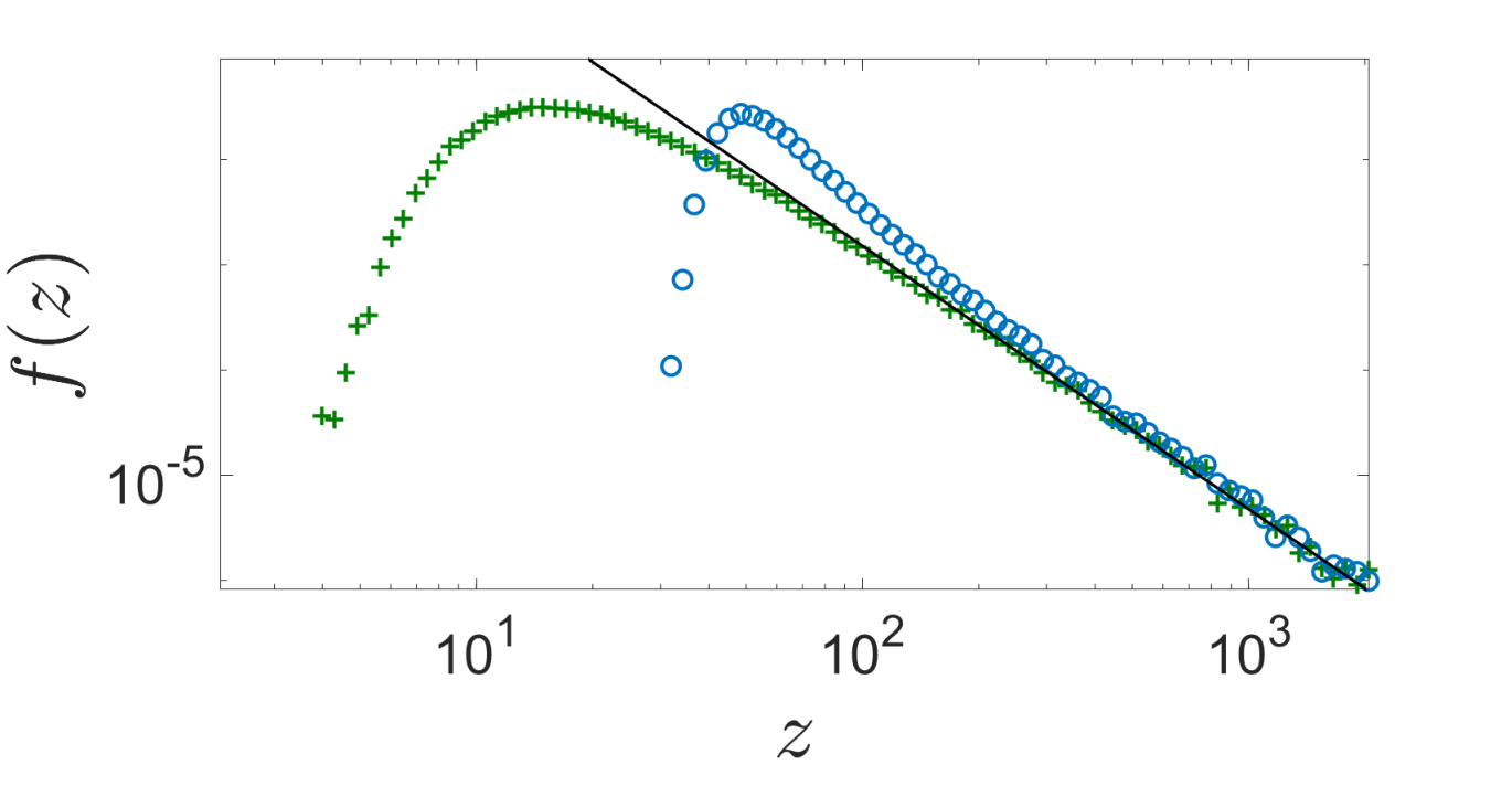
The unconditional cumulative distribution function (CDF) of the maximum is per definition

i.e. every increment $\tilde{\delta}_{i}$ is less or equal than the value $z$. In particular, here, it is irrelevant which increment is the maximum. Here and only in this subsection, we add $N$ in the argument of $F_{\tilde{\delta}_{\text{max}}}(z;N)$ to highlight the $N$-dependence. We always assume $N$ to be finite.

We show in App. D for the case with a power law PDF $f_{\delta_{i}}(z)\sim Az^{-1-\alpha}$ that the large $z$ behaviour of $F_{\tilde{\delta}_{\text{max}}}(z;N)$ is given by the product

For $N=2$ we have clearly a multiplication of two CDFs just like the IID case. This was precisely the point in previous Sec. IV. Generally, the formula Eq. (29), which is valid only for large $z$, is similar the IID case where the well-known maximum CDF $F_{\delta_{\text{max}}}(z;N)=[F_{\delta_{i}}(z)]^{N}$ describes the maximum of the $N$ IID random variables $\delta_{i}$. However, in the correlated case, only the first increment $\tilde{\delta}_{1}=\delta_{1}$ has the same statistical properties as those of the IID process. This gives the term $F_{\delta_{i}}(z)$ in Eq. (29). The following $N-1$ increments $\tilde{\delta}_{i}$, $i\geq 2$, are correlated and therefore are governed by the term $F_{\tilde{\delta}_{\text{max}}}(z;N-1)$ instead of $F_{\delta_{\text{max}}}(z;N-1)=[F_{\delta_{i}}(z)]^{N-1}$.

The maximum PDF is the derivative $f_{\tilde{\delta}_{\text{max}}}(z;N)=\mathrm{d}/\mathrm{d}zF_{\tilde{\delta}_{\text{max}}}(z;N)$ and therefore

Here, we used that both CDFs $F_{\tilde{\delta}_{\text{max}}}(z;N-1)$ and $F_{\delta_{i}}(z)$ are about $1$ for large $z$. Thus, we can deduce (proof by induction) that the tail of the maximum increment PDF follows

which is the same as the tail of $f_{\delta_{\text{max}}}(z;N)$ describing the maximum of the IID random variables. Summarized, we can say that

for large $z$, see Fig. 4. This formula is the general statement of the exemplary results of Eq. (25).

In Fig. 5, we present the scatter plot between $\tilde{\delta}_{\text{max}}$ and $\delta_{\text{max}}$ for the algebraical memory kernel for two different PDFs of $\delta_{i}$, namely the two-sided symmetric Lévy PDF and the Pareto PDF. For the first example, we observe a straight line for large values $\tilde{\delta}_{\text{max}}\approx\delta_{\text{max}}$. But for the second example, we see some offset $\tilde{\delta}_{\text{max}}\approx\delta_{\text{max}}+C$. The reason for that is the correction to the BJP which we already found for the IID case, see Sec. II and App. A. We can find the offset $C$ here by replacing the remaining random (which are not the maximum) variables by their mean, see details for the correlated random walk also in App. A. Let’s say $\tilde{\delta}_{\text{max}}$ happens at b so that $\tilde{\delta}_{\text{max}}=\tilde{\delta}_{b}$. Per definition, the $b$-th increment is $\tilde{\delta}_{b}=\delta_{b}+\sum_{j=1}^{b-1}M_{b-j}\delta_{j}$. Assuming $\delta_{b}$ is large, we claim $\tilde{\delta}_{b}\stackrel{{\scriptstyle d}}{{\sim}}\delta_{b}+\langle\delta_{i}\rangle\sum_{j=1}^{b-1}M_{b-j}$. This formula is conditioned on the step number $b$. Now we average over $b$. Thus, we get the unconditional relationship $\tilde{\delta}_{\text{max}}\stackrel{{\scriptstyle d}}{{\sim}}\delta_{\text{max}}+C$ with the offset $C=\langle\delta_{i}\rangle\sum_{b=1}^{N}\left[\Phi(b)\sum_{j=1}^{b-1}M_{b-j}\right]$. The probability $\Phi(b)$ that $\tilde{\delta}_{\text{max}}$ appears at $b$ will be discussed below when we study the conditional BJP. In Fig. 5, the offset $C$ is visible in the scatter plot for the Pareto case because small $\beta$ and large $N$ lead to a large $C$. If we would sample more data, we eventually would find even larger maxima so that the offset will be less visible in the scatter plot. But even for small $C$ we find that this correction describes well also other distributions of this work at hand. In App. A, we present the correction terms for the conditional and unconditional sum and maximum distributions.

We already calculated the unconditional PDF of $\tilde{x}_{N}$ when the IID random variables $\delta_{i}$ follow the symmetric Lévy PDF, see Eq. (12). We also found the PDF of $\tilde{x}_{N}$ for the Pareto case when $N\to\infty$, see Eq. (16). Hence, we are left with the Pareto case when $N$ is finite which we perform now.

The unconditional PDF of the sum $\tilde{x}_{N}$ is the $N$-fold convolution

The effect of correlations enters in this equation through the factors $W_{N-1},\ldots,W_{0}$. The $2$-fold convolution is defined as $(f\ast g)^{(2)}(z)=\int_{0}^{z}f(x)g(z-x)\mathrm{d}x$ and higher orders subsequently. We calculate the Laplace transform $\hat{f}_{\tilde{x}_{N}}(s)=\int_{0}^{\infty}f_{\tilde{x}_{N}}(z)\text{exp}(-zs)\mathrm{d}z$. The $N$-fold convolution is in Laplace space the $N$-product

The small $s$ behaviour of the Laplace transform for the increment Pareto PDF is $\hat{f}_{\delta_{i}}(s)\sim 1+\alpha\Gamma(-\alpha)s^{\alpha}$ when $\alpha\in(0,1)$ and $\hat{f}_{\delta_{i}}(s)\sim 1-\langle\delta_{i}\rangle s+\alpha\Gamma(-\alpha)s^{\alpha}$ when $\alpha\in(1,2)$. Therefore, we find the large sum behaviour given by the small $s$ expansion $\hat{f}_{\tilde{x}_{N}}(s)\sim\alpha\Gamma(-\alpha)\tilde{\gamma}_{N}s^{\alpha}$ for both $\alpha\in(0,1)$ and $\alpha\in(1,2)$ with the scaling factor $\tilde{\gamma}_{N}=\sum_{i=1}^{N}(W_{N-i})^{\alpha}$ (see Eq. (13)). Inverse Laplace transform $s\to z$ gives the large z behaviour

We finally have all results to state the unconditional BJP.

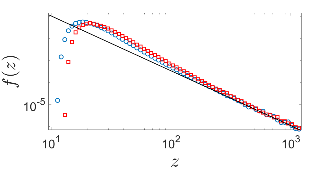
We compare the tail of the maximum distribution of Eq. (31) with the tail of the sum distributions of Eq. (12) and (35). We find the unconditional BJP

for large $z$ and any $N$. We presented it earlier in Eq. (21). This formula implies the random variable transform

for large values because $f_{\left(\tilde{\gamma}_{N}/N\right)^{1/\alpha}\tilde{\delta}_{\text{max}}}(z)\sim(\tilde{\gamma}_{N}/N)f_{\tilde{\delta}_{\text{max}}}(z)$. In Fig. 6 we compare the theory of Eq. (36) with Monte-Carlo simulations and find perfect agreement.

We present an alternative argumentation to find the conditional BJP. The interesting point here is that we can use the IID BJP and find easily the conditional BJP without long calculations. In some sense, this alternative discussion here is a generalisation of Sec. IV. Most results in this subsection were shown previously. However, one particular point becomes clearer now, namely the behaviour of the subsequent increments after the big jump.

We rearrange the definition of the sum $\tilde{x}_{N}=\sum_{i=1}^{N}\left(\sum_{j=1}^{i}M_{i-j}\delta_{j}\right)$ according to

i.e. the correlated sum $\tilde{x}_{N}$ is written in terms of a weighted sum of the uncorrelated sum $x_{N}$. Let’s assume that the maximum of the IID random variables $\delta_{\text{max}}$ happens at step number $b$ and is also large. This is the condition on the appearance of $\delta_{\text{max}}$ and not $\tilde{\delta}_{\text{max}}$. This implies $x_{N-l}\stackrel{{\scriptstyle d}}{{\sim}}\delta_{\text{max}}$ for $N-l\geq b$ which is the IID BJP of Eq. (1). Thus, Eq. (42) becomes

where the terms with $N-l<b$ can be neglected. This is Eq. (41).

Eq. (43) has an important implication, namely all increments with $i\geq b$ are statistically described by a single term

This is a relation between the $i$-th increment $\tilde{\delta}_{i}$ with $i=b,\ldots,N$ and the maximum of the noise increments $\delta_{\text{max}}=\delta_{b}$. Eq. (44) can be seen by comparison of the prefactors between Eq. (43) and the definition $\tilde{\delta}_{i}=\sum_{j=0}^{i}M_{i-j}\delta_{j}$. Thus, the sum $\sum_{j=0}^{i}M_{i-j}\delta_{j}$ is solely described by the single term $M_{b-i}\delta_{\text{max}}$ which is influenced by the big jump directly and all other summands can be neglected. Based on Eq. (44), we find three key points under the assumption of large $\delta_{\text{max}}$:

• 1)

  The big jump is statistically the same as the maximum of the IID random variables $\tilde{\delta}_{\text{max}}\stackrel{{\scriptstyle d}}{{\sim}}\delta_{\text{max}}$ when both are large.

• 2)

  The increments following the big jump can never be neglected when summing up to $\tilde{x}_{N}$.

• 3)

  The correlated sum conditioned on $b$ is statistically $\tilde{x}_{N}\stackrel{{\scriptstyle d}}{{\sim}}W_{N-b}\tilde{\delta}_{\text{max}}$ when both sides are large.

In particular, the third point is the conditional BJP of Eq. (40).

We have seen how the interplay between big jump and correlations lead to the conditional BJP. Let’s conclude this observation with another implication. Take the example of the IID random variables following the Pareto PDF $f_{\delta_{i}}(z)$. The non-negligible subsequent increments after the big jump lead to an amplification of the sum $\tilde{x}_{N}$ compared to $x_{N}$. We demonstrate this in Fig. 11 for the two memory kernels. The earlier the big jump happened the bigger is the influence of the big jump on the random walk due to the correlations. In other words, once a very large maximum occurred we can predict the future since the future depends only on the big jump (from the past) and the deterministic value of the correlation.

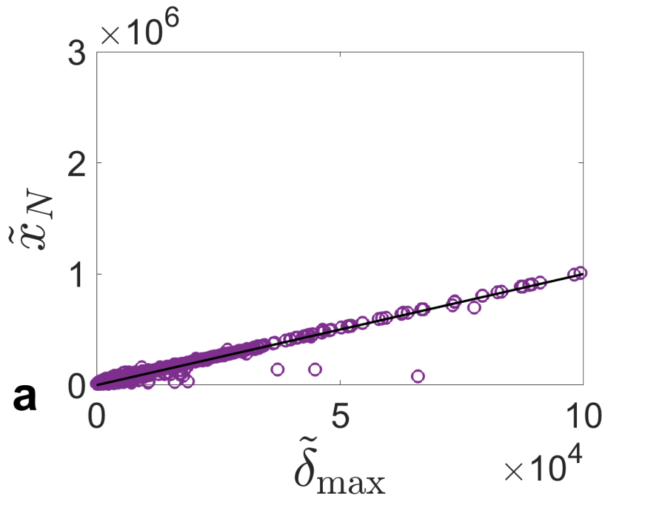
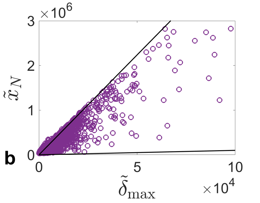
In Fig. 12, we present the scatter plot between $\tilde{\delta}_{\text{max}}$ and $\tilde{x}_{N}$ for the large value of $N=500$. We present the exponential and algebraical memory kernel case. For both cases, we don’t see $N$ lines as in the scatter plots of Fig. 2 and 10 where we present small $N$. The reason is simply that we don’t have enough realizations which are necessary to sample the rare events. Furthermore, we observe two different behaviours between the exponential and algebraical memory case. While exponential case yields a straight line, the algebraical case looks like a triangle. This is because the weight $W_{N-b}$ for large $N$ either converges (exponential memory) or not (algebraical memory). Here, it is important that we don’t fix $b$ as previously in Eq. (10) and (11). We explain now both cases in detail.

For the exponential memory, we still can use the large $N$ behaviour of Eq. (10), namely $W_{N-b}\sim 1/(1-m)$, even when we don’t fix $b$. The latter is important. For large $N$ only values $b\approx N$ yield $W_{N-b}\not\sim 1/(1-m)$. But this amount of $W_{N-b}$ is negligible to those $W_{N-b}$ which behave as $1/(1-m)$. So we get the conditional BJP of Eq. (40) for large $N$ as

for large $z$. The prefactor in the right hand side doesn’t depend on $b$. So this is also the unconditional BJP for large $N$ which we can show directly. When we take the large $N$ limit of the prefactor $\tilde{\gamma}_{N}/N$ in the unconditional BJP Eq. (36), we find again Eq. (45) but now not conditioned on $b$. The variable transform of Eq. (45) is

under the assumption of large $N$. The prefactor $1/(1-m)$ is the slope we observe in the scatter plot of Fig. 12.

In contrast, for the algebraical memory kernel, the weight $W_{N-b}$ for large $N$ but not fixed $b$ cannot be replaced by $N^{1-\beta}/(1-\beta)$. The latter assumes fixed $b$, see Eq. (11). For large $N$, there is a non-negligible amount of $W_{N-b}$ which is not similar to this limit. And this is what we observe in the scatter plot. It is statistically difficult to observe $N$ lines because it would require a tremendous amount of realizations of $\tilde{x}_{N}$. What one observe instead for a large but finite amount of realizations is a triangle structure confined by the lowest and largest slope

References

- (1) V. P. Chistyakov, Theory Probab. Its Appl. 9, 640 (1964).
- (2) T. Mikosch and O. Wintenberger, Probability Theory and Related Fields 166, 233 (2016).
- (3) D. G. Konstantinides, T. Mikosch, et al., The Annals of Probability 33, 1992 (2005).
- (4) T. Mikosch and G. Samorodnitsky, Annals of Applied Probability 1025–1064 (2000).
- (5) P. Embrechts and N. Veraverbeke, Insur. Math. Econ. 1, 55 (1982).
- (6) T. Rolski, H. Schmidli, V. Schmidt, and J. L. Teugels, Stochastic processes for insurance and finance (John Wiley & Sons, 2009).
- (7) A. E. Kyprianou, Introductory lectures on fluctuations of Lévy processes with applications (Springer Science & Business Media, 2006).
- (8) A. Vezzani, E. Barkai, and R. Burioni, Phys. Rev. E 100, 012108 (2019).
- (9) W. Wang, A. Vezzani, R. Burioni, and E. Barkai, Phys. Rev. Res. 1, 033172 (2019).
- (10) R. Burioni and A. Vezzani, J. Stat. Mech. Theory Exp. 2020, 034005 (2020).
- (11) A. Vezzani, E. Barkai, and R. Burioni, Sci. Rep. 10, 1 (2020).
- (12) W. Wang, M. Höll, and E. Barkai, Physical Review E 102, 052115 (2020).
- (13) S. N. Majumdar, A. Pal, and G. Schehr, Phys. Rep. 840, 1 (2020).
- (14) C. Godrèche, J. Phys. A Math. Theor. 50, 195003 (2017).
- (15) C. Godrèche, J. Stat. Phys. 182, 1 (2021).
- (16) M. Höll, W. Wang, and E. Barkai, Phys. Rev. E 102, 042141 (2020).
- (17) A. Bar, S. N. Majumdar, G. Schehr, and D. Mukamel, Phys. Rev. E 93, 052130 (2016).
- (18) F. Mori, S. N. Majumdar, and G. Schehr, arXiv preprint arXiv:2104.07346 (2021).
- (19) D. S. Grebenkov, V. Sposini, R. Metzler, G. Oshanin, and F. Seno, New J. Phys. 23, 023014 (2021).
- (20) M. M. Meerschaert, E. Nane, and Y. Xiao, Statistics & Probability Letters 79, 1194 (2009).
- (21) A. V. Chechkin, M. Hofmann, and I. M. Sokolov, Physical Review E 80, 031112 (2009).
- (22) J. H. Schulz, A. V. Chechkin, and R. Metzler, Journal of Physics A: Mathematical and Theoretical 46, 475001 (2013).
- (23) V. Tejedor and R. Metzler, Journal of Physics A: Mathematical and Theoretical 43, 082002 (2010).
- (24) M. Montero and J. Masoliver, Phys. Rev. E 76, 061115 (2007).
- (25) A. Comolli and M. Dentz, Phys. Rev. E 97, 052146 (2018).
- (26) D. S. Johnson, J. M. London, M.-A. Lea, and J. W. Durban, Ecology 89, 1208 (2008).
- (27) A. Maye, C.-h. Hsieh, G. Sugihara, and B. Brembs, PloS one 2, e443 (2007).
- (28) M. Magdziarz, R. Metzler, W. Szczotka, and P. Zebrowski, Physical Review E 85, 051103 (2012).
- (29) P. De Anna, T. Le Borgne, M. Dentz, A. M. Tartakovsky, D. Bolster, and P. Davy, Phys. Rev. Lett. 110, 184502 (2013).
- (30) J. Janczura, S. Orzeł, and A. Wyłomańska, Physica A: Statistical Mechanics and its Applications 390, 4379 (2011).
- (31) H. Fink, C. Klüppelberg, et al., Bernoulli 17, 484 (2011).
- (32) T. Mikosch, T. Gadrich, C. Kluppelberg, and R. J. Adler, The Annals of Statistics 305–326 (1995).
- (33) J. Liu, S. Kumar, and D. P. Palomar, IEEE Transactions on Signal Processing 67, 2159 (2019).
- (34) G. Samoradnitsky, Stable non-Gaussian random processes: stochastic models with infinite variance (Routledge, 2017).
- (35) P. Embrechts, C. Klüppelberg, and T. Mikosch, Modelling Extremal Events: for Insurance and Finance, vol. 33 (Springer Verlag, Berlin Heidelberg, 2013).
- (36) K. Burnecki and A. Weron, Physical Review E 82, 021130 (2010).
- (37) K. Burnecki and G. Sikora, Chaos, Solitons & Fractals 102, 456 (2017).
- (38) B. Dybiec, E. Gudowska-Nowak, and P. Hänggi, Phys. Rev. E 73, 046104 (2006).
- (39) B. Dybiec, E. Gudowska-Nowak, and P. Hänggi, Phys. Rev. E 75, 021109 (2007).
- (40) H. Hilhorst, Braz. J. Phys. 39, 371 (2009).
- (41) E. Bertin and M. Clusel, J. Phys. Math. Gen. 39, 7607 (2006).
- (42) F. Baldovin and A. L. Stella, Phys. Rev. E 75, 020101 (2007).
- (43) B. Berkowitz and H. Scher, Phys. Rev. E 81, 011128 (2010).
- (44) S. M. Papalexiou and D. Koutsoyiannis, Water Resour. Res. 49, 187 (2013).