Diffusion of gravity waves by random space inhomogeneities in pancake-ice fields.
Theory and validation with wave buoys and SARPreprint: AIP/123-QED

P. Olla Also at INFN, Sez. Cagliari, I–09042 Monserrato, Italy Email: olla@dsf.unica.it Affiliation: ISAC-CNR Sez. Cagliari, I–09042 Monserrato, Italy G. De Carolis Affiliation: IREA-CNR, Sez. Milano, I–20133 Milano, Italy F. De Santi Affiliation: IREA-CNR, Sez. Milano, I–20133 Milano, Italy

August 11, 2026

Abstract

We study the diffusion of ocean waves by ice bodies much smaller than a wavelength, such as pancakes and small ice floes. We argue that inhomogeneities in the ice cover at scales comparable to that of the wavelength significantly increase diffusion, producing a contribution to wave attenuation comparable to what it is observed in the field and usually explained by viscous effects. The resulting attenuation spectrum is characterized by a peak at the scale of the inhomogeneities in the ice cover, which could explain the rollover of the attenuation profile at small wavelengths observed in field experiments. The proposed attenuation mechanism leads to the same behaviors that would be produced by a viscous wave model with effective viscosity linearly dependent on the ice thickness. This may explain recent findings that viscous wave models require a thickness-dependent viscosity to fit experimental attenuation data. Experimental validation is carried out using wave buoy attenuation data and SAR image analysis.

I Introduction

Ocean surface waves play an important role in the dynamics of sea ice in polar regions. The effect is particularly visible in the Marginal Ice Zone (MIZ);, which is the highly dynamical transition region separating the ice pack from the open oceanSquire 1995. In the summer season, erosion of the pack and breakup of large flows into smaller ice bodies, are the dominant processes in the region. During winter, waves infiltrating the MIZ contribute to ice formation through the coalescence of ice bodies into progressively larger objects Thomson and Rogers 2014. Global warming has led to an increase in both the activity and the extension of the MIZ. The Arctic in particular has seen a dramatic summertime increase of the MIZ extension and a concomitant reduction of the ice surface Parkinson and Comiso 2013; Thomson et al. 2018. To determine how deep ocean waves can propagate into the MIZ, one must know the sea ice contribution to wave damping. Over the years, a great effort has been put into studyng the modifications in surface waves propagation induced by sea ice (see Squire Squire 1995; Squire 2007; Squire 2020 for an extended review). In particular, remote sensing analysis of the modifications to wave propagation by sea ice has been used as a tool to infer the ice thickness without having to resort to in situ measurements Wadhams et al. 1999; De Carolis 2001; Wadhams, Parmiggiani, and De Carolis 2002; De Carolis 2003; Wadhams et al. 2004; Sutherland and Gascard 2016; Wadhams et al. 2018; De Carolis, Olla, and De Santi 2021.

Wave attenuation depends on the characteristic size of the ice bodies involved. In the case of larger floes on the scale of tens to hundreds of meters, scattering and diffraction Masson and LeBlond 1989; Bennetts and Squire 2012, as well as flexural deformations of the floes Meylan and Squire 1996; Meylan et al. 2015, are expected to dominate (see Li, Shi, and Wu 2021 for a recent application of thin plate theory to wave propagation in water covered by a continuous ice sheet). On the other hand, in the case of smaller ice bodies, viscous effects and collisions are expected to be dominant. Kohout and Meylan 2008; Squire and Montiel 2016. The picture is complicated by the strong inhomogeneity of the MIZ; although small ice is prevalent at the fringes of the MIZ, ice bodies of widely different sizes and typology can be found anywhere in the region Toyota, Haas, and Tamura 2011.

The focus of the present paper is the modification of ocean wave propagation produced by ice bodies much smaller than a wavelength, in particular pancake-ice. Pancake-ice is the assembly of pancake-shaped ice bodies of diameters ranging from 30 centimeters to 3 meters, which populate, during ice formation, the outer fringes of the MIZ Doble, Coon, and Wadhams 2003; Doble et al. 2015. It usually comes as a component of so-called grease-pancake ice (GPI), i.e. pancake-ice embedded in a dense slurry of ice crystals, called grease ice.

Grease ice is a strongly viscous medium, which is usually treated as a viscous continuum Keller 1998. Over the years various extensions of the viscous model have been proposed, such as the inclusion of viscoelasticity in the ice response Wang and Shen 2010; Chen, Gilbert, and Guyenne 2019 and of turbulent effects in the water under the ice De Carolis and Desiderio 2002, and the treatment of pancakes as an individual layer separate from grease ice De Santi and Olla 2017.

Providing a microscopic explanation for the effective viscosity of GPI, however, has proven problematic. This is reflected in the wide variation of the values of the parameter required to fit different experimental data sets Cheng et al. 2017; De Santi et al. 2018. The difficulty is compounded by recent observations De Carolis, Olla, and De Santi 2021; Sutherland et al. 2019; Doble et al. 2015; Li et al. 2017 that most viscous layer models require an effective viscosity dependent on the ice thickness to fit available experimental data. The possibility that an intensive quantity such as the ice viscosity depends on a macroscopic quantity such as the ice layer thickness casts doubts on whether GPI could be treated as a simple viscous medium. Besides, there are situations in which pancakes (or other forms of multi-year small scale or brash ice) float in low-viscosity grease-ice-free water Thomson et al. 2018.

Another difficulty is that current viscous models are unable to explain the rollover effect, i.e. the decrease of wave attenuation at short wavelengths which is often observed in field measurements. Although this phenomenon has been discussed for over four decades, it still lacks of an exhaustive explanation.The rollover effect has been so far ascribed to instrumental noise Thomson et al. 2020, to exogenous mechanisms not properly taken into account, such as the energy input by the wind Li et al. 2017, and to the effect of nonlinearities Polnikov and Lavrenov 2007. A possible explanation of the phenomenon was proposed by Liu and Mollo-Christensen 1988 as the result of the development of a viscous boundary layer under a continuous ice sheet treated as a thin elastic plate. Another explanation of the phenomenon was proposed by Perrie and Hu 1996, who performed numerical simulations with constant wind and regular arrays of medium size circular ice floes (diameter $20\,{\rm m}$ ), suggesting that rollover is indeed the result of wave scattering. To our knowledge, however, scattering theory has never been applied at pancake scales yet.

All these remarks call for a reappraisal of alternative mechanisms of wave attenuation, such as, e.g., collisions between ice bodies Shen and Squire 1998, nonlinear forces and turbulence induced in the surrounding water by the ice motion Skene et al. 2015.

Purpose of the present study is to evaluate the scattering contribution to wave attenuation. We show that random inhomogeneities in the ice cover generate a coherent scattering component that can contribute significantly to wave damping. The phenomenon is akin to the enhancement of light scattering in a turbid medium. The approach we are going to follow is common to that for larger floes, and is based on partial wave expansion of the flow disturbances generated by the inhomogeneities of the ice cover Kagemoto and Yue 1986. The nature of the scattering process in the case of floating bodies much smaller than a wavelength, however, is fundamentally different, as bodies within a wavelength respond coherently to the wave, and subtle near-field effects simplify the treatment of the scattering dynamics.

We assume potential flow for both the incident wave and the disturbances, thus disregarding viscous effects from the possible presence of grease ice at the water surface. Small amplitude waves and linear hydrodynamics are assumed throughout the analysis; for simplicity, only the case of deep water waves is considered. We treat the ice layer as an inextensible continuum with vanishing resistance to bending and with a rough bottom. In the case of a spatially uniform layer and no roughness, the dynamics reduce to that of the mass-loading model Peters 1950; Keller and Weitz 1953.

We compare our theoretical results with experimental data from wave buoys collected during the Sikuliaq campaign in Autumn 2015 Thomson et al. 2018. By exploiting the availability of attendant satellite SAR images available, it is possible to estimate the scale of the ice cover spatial inhomogeneities, which appears to coincide with that of the rollover peak.

The paper is organized as follows. In Sec. II, the general theory of scattering of gravity waves by floating bodies is reviewed. In Secs. III and IV, we apply the theory to determine the modification to the wavefield generated by random spatial variations in a continuous cover. In Sec. V, the consequences of the results on wave attenuation are discussed. In Sec. VI, the specific example of a spatially inhomogeneous mass loading with a rough ice-water interface, is considered. In Section VII, current results are contextualized to the others wave propagation models in the literature. Section VIII contains a comparison with experimental data. Concluding remarks are reported in Section IX.

II Partial wave expansion

The study of the scattering of ocean waves by solid obstacles has a long history, which makes extensive use of techniques drawn from the study of similar problems in electromagnetism, acoustics and quantum mechanics. The approach has been detailed elsewhere (see e.g. Peter and Meylan 2004a). We outline here the essentials.

The wave dynamics obeys the linearized Euler equation

\displaystyle\rho\partial_{t}{\bf U}+\nabla P=0,\quad\nabla\cdot{\bf U}=0,

(1)

where ${\bf U}({\bf x},t)$ is the fluid velocity, $\rho\simeq 1025\ {\rm kg\,m^{-3}}$ is the salt water density, $P({\bf x},t)$ is the deviation of the pressure in the water column from its value at hydrostatic equilibrium, and we have put the unperturbed water surface at $x_{3}=0$ with ${\bf e}_{3}$ pointing upwards. Equation (1) implies potential flow

\displaystyle{\bf U}=-\nabla\Phi,\qquad\nabla^{2}\Phi=0.

(2)

Continuity of the pressure at the water surface, $P({\bf x}(t),t)|_{x_{3}=0}=0$ , where ${\bf x}(t)$ is the instantaneous position of the point at the water-atmosphere interface, leads to the boundary condition on Eq. (2)Landau and Lifshitz 1987

\displaystyle\Big(\frac{\partial^{2}\Phi}{\partial t^{2}}+g\frac{\partial\Phi}{\partial x_{3}}\Big)_{x_{3}=0}=0.

(3)

The wave energy contains both potential and kinetic energy contributions. We can eliminate the potential energy component by averaging over a suitable time window $w$ , and thus get the expression for the time averaged wave energy density

\displaystyle\mathcal{E}_{\Phi}({\bf x}_{\perp},t)

\displaystyle=

\displaystyle\frac{\rho}{2}\int_{-\infty}^{0}{\rm d}x_{3}\ \langle|{\bf U}({\bf x},t)|^{2}\rangle_{w},

(4)

where ${\bf x}=({\bf x}_{\perp},x_{3})$ and $\langle.\rangle_{w}$ indicates time average in $w$ . By comparing Eq. (4) with Eqs. (2) and (3) we find the conservation law

\displaystyle\partial_{t}\mathcal{E}_{\Phi}+\nabla_{\perp}\cdot{\bf J}_{\Phi}=0,\qquad{\bf J}_{\Phi}({\bf x}_{\perp},t)=\int_{-\infty}^{0}{\rm d}x_{3}\ \langle P({\bf x},t){\bf U}_{\perp}({\bf x},t)\rangle_{w}.

(5)

We assume elastic scattering, which implies linearity of possible mechanical interactions of the floating bodies; linear hydrodynamics then implies that the scattered waves oscillate with the same frequency of the incident wave. In the case of a monocromatic incident wave of frequency $\omega$ , the energy current ${\bf J}_{\Phi}$ will satisfy

\displaystyle{\bf J}_{\Phi}={\rm i}\rho\omega\int_{-\infty}^{0}{\rm d}x_{3}\ [\Phi\nabla_{\perp}\Phi^{*}-\Phi^{*}\nabla_{\perp}\Phi].

(6)

We are interested in the scattering by ice bodies of characteristic size $R$ much less than a wavelength. Taking inspiration from the treatment of similar problems in the case of electromagnetic radiation Jackson 1999, we separate in the potential a near-field component $\phi$ from disturbances from bodies at distance $\ll k^{-1}$ from ${\bf x}$ , and a remnant $\Psi$ containing the incident and the diffused waves:

\displaystyle\Phi({\bf x},t)=\Psi({\bf x},t)+\phi({\bf x},t).

(7)

A summary of the relevant scales in the problem is provided in Table 1.

Table 1: Relevant scales of the problem

Near field $kL\ll 1$	Pancake scale $L\sim R$ .	Pancake geometry important.
Near field $kL\ll 1$	Intermediate scale $L\gg R$ .	Multipole expansion approach.
Wave region $kL\sim 1$	Perturbations acquire a wave character —	assumed scale of ice inhomogeneities ( $\lambda$ ).
Far field $kL\gg 1$	Diffused waves.

We are interested in the scattering by random space inhomogeneity of the ice cover. Let us then indicate with overbar the operation of ensemble average with respect to the homogeneities of the ice cover and with tilde fluctuation, and decompose the generic physical quantity $f$ accordingly:

\displaystyle f=\bar{f}+\tilde{f}.

(8)

Hence $\bar{\Psi}$ contains the incident wave, $\tilde{\Psi}$ contains the diffused waves; ensemble averaging and coarse-graining have the same filtering effect on the small scales, therefore $\bar{\Phi}=\bar{\Psi}$ and $\phi=\tilde{\phi}$ .

Refer to caption — Figure 1: Geometry of the problem

Consider a portion $A$ of unperturbed water surface at ${\bf x}_{\perp}=0$ and indicate with $\tilde{\Psi}_{A}$ the contribution to wave diffusion from the bodies in that region.The geometry of the problem is sketched in Fig. 1. Let us assume a monocromatic incident wave propagating to positive $x_{1}$ : ${\bf k}=k{\bf e}_{1}$ ; from Eqs. (2) and (3) we then get the classical deep-water surface gravity wave solution in ice-free water

\displaystyle\bar{\Psi}({\bf x},t)=\bar{\Psi}_{0}(t)\exp(kx_{3}+{\rm i}kx_{1})=\bar{\Psi}_{0}\exp[kx_{3}+{\rm i}(kx_{1}-\omega t)],\quad\omega^{2}=kg.

(9)

We can expand the incident wave in partial waves

\displaystyle\bar{\Psi}({\bf x},t)=\bar{\Psi}(t)\Big[J_{0}(kx_{\perp})+2\sum_{n=1}^{\infty}{\rm i}^{n}J_{n}(kx_{\perp})\cos(n\varphi)\Big]{\rm e}^{kx_{3}},

(10)

and similarly for $\Psi_{A}=\bar{\Psi}+\tilde{\Psi}_{A}$ ,

	$\displaystyle\Psi_{A}({\bf x},t)$	$\displaystyle=$	$\displaystyle\tilde{\Psi}_{A,eva}({\bf x},t)+\bar{\Psi}_{0}(t)\Big[B_{0}J_{0}(kx_{\perp})+C_{0}N_{0}(kx_{\perp})$		(11)
		$\displaystyle+$	$\displaystyle 2\sum_{n=1}^{\infty}{\rm i}^{n}\Big(B_{n}J_{n}(kx_{\perp})+{\rm i}C_{n}N_{n}(kx_{\perp})\Big)\cos(n\varphi)\Big]{\rm e}^{kx_{3}},$		(11)

where $\cos\varphi=x_{1}/x_{\perp}$ , $J_{n}$ and $N_{n}$ are Bessel functions of the first and second kind, respectively, and $\tilde{\Psi}_{A,eva}$ contains evanescent modes, which can be expressed in terms of modified Bessel functions $K_{n}$ , exponentially decaying at large $kx_{\perp}$ Abramowitz, Stegun, and Romer 1988. The evanescent modes can be disregarded in the far-field region, and the remaining part of $\Psi_{A}$ is a sum of outward and inward propagating modes $\propto{\rm e}^{\pm{\rm i}kx_{\perp}}$ . Requiring $\tilde{\Psi}_{A}$ not to contain inward propagating modes (Sommerfeld condition), together with stationarity, ${\bf J}_{\bar{\Psi}}=0$ , allows us to fix the coefficients in Eq. (11) Landau and Lifshitz 2013. This gives us the expression for the perturbed field in the far-field region $kx_{\perp}\gg 1$

	$\displaystyle\tilde{\Psi}_{A}({\bf x},t)$	$\displaystyle=$	$\displaystyle\bar{\Psi}_{0}(t)\Big[\frac{{\rm e}^{2{\rm i}\delta_{A,0}-1}}{2}H_{0}^{\scriptscriptstyle(1)}(kx_{\perp})+\sum_{n=1}^{\infty}{\rm i}^{n}({\rm e}^{2{\rm i}\delta_{A,n}}-1)$		(12)
		$\displaystyle\times$	$\displaystyle H_{n}^{\scriptscriptstyle(1)}(kx_{\perp})\cos(n\varphi)\Big]{\rm e}^{kx_{3}},\qquad\quad kx_{\perp}\gg 1,$		(12)

where $H^{\scriptscriptstyle(1)}_{n}=J_{n}+{\rm i}N_{n}$ are Hankel function of the first kind Abramowitz, Stegun, and Romer 1988, and the coefficients $\delta_{A,n}$ are real constants called the scattering phases.

We confine our attention to situations in which scattering can be considered a perturbation; the scattering phases therefore are small and we can linearize Eq. (12):

	$\displaystyle\tilde{\Psi}_{A}({\bf x},t)$	$\displaystyle\equiv$	$\displaystyle\sum_{n}\tilde{\Psi}_{A,n}({\bf x},t)\simeq{\rm i}\bar{\Psi}_{0}(t)\Big[\delta_{A,0}H_{0}^{\scriptscriptstyle(1)}(kx_{\perp})$		(13)
		$\displaystyle+$	$\displaystyle 2\sum_{n=1}^{\infty}{\rm i}^{n}\delta_{A,n}H_{n}^{\scriptscriptstyle(1)}(kx_{\perp})\cos(n\varphi)\Big]{\rm e}^{kx_{3}},\qquad kx_{\perp}\gg 1.$		(13)

Let us suppose that $A$ contains all the bodies responsible for scattering, or equivalently that the interference with waves scattered by bodies outside $A$ is negligible. In this case, the radiated energy is

\displaystyle I_{\tilde{\Psi}_{A}}=\int_{0}^{2\pi}{\rm d}\varphi\ {\bf x}_{\perp}\cdot{\bf J}_{\tilde{\Psi}_{A}}({\bf x}),

(14)

where $J_{\tilde{\Psi}_{A}}$ is obtained from Eq. (6) by replacing $\Phi$ with $\tilde{\Psi}_{A}$ . Substituting Eq. (13) into Eq. (14) and exploiting the relation $N^{\prime}_{n}(z)J_{n}(z)-N_{n}(z)J^{\prime}_{n}(z)=2/(\pi z)$ Abramowitz, Stegun, and Romer 1988 yields

\displaystyle I_{\tilde{\Psi}_{A}}\equiv\sum_{n}I_{\tilde{\Psi}_{A,n}}=\int_{0}^{2\pi}{\rm d}\varphi\ {\bf x}_{\perp}\cdot{\bf J}_{\tilde{\Psi}_{A}}({\bf x})\simeq\frac{4\rho\omega|\bar{\Psi}_{0}|^{2}}{k}\sum_{n=0}^{\infty}\delta^{2}_{A,n}.

(15)

By combining Eq. (15) with the energy flux density of the incident wave

\displaystyle{\bf J}_{\bar{\Psi}}=\omega\rho|\bar{\Psi}_{0}|^{2}{\bf e}_{1},

(16)

we obtain the expression for the scattering cross-section

\displaystyle\sigma_{A}=\frac{I_{\tilde{\Psi}_{A}}}{J_{\bar{\Psi}}}\simeq 4k^{-1}\sum_{n=0}^{\infty}\delta_{A,n}^{2}.

(17)

III The near field

Let us consider a region $A$ at the water surface around $x_{\perp}=0$ , of size $L_{A}$ sufficiently large to carry out a continuous limit, but small compared to the wavelength: $R\ll L_{A}\ll k^{-1}$ . The near-field disturbance by the bodies in $A$ is a complicated superposition of propagating and evanescent modes Kagemoto and Yue 1986; Peter and Meylan 2004b, which is more aptly analyzed by making the decomposition $\phi_{A}=\phi_{A,reg}+\phi_{A,sing}$ , where $\phi_{A,reg}$ and $\phi_{A,sing}$ , are the regular (singular) components of $\phi$ at ${\bf x}_{\perp}=0$ , $R,L\to 0$ , and both components are required to decay for $x_{\perp}\to\infty$ .

The regular component can only contain Bessel functions $J_{n}$ . We therefore obtain from Eq. (13) the expression, valid for all $kx_{\perp}$ ,

\displaystyle\phi_{A,reg}\equiv\sum_{n}\phi_{A,reg,n}\simeq{\rm i}\bar{\Psi}_{0}\Big[\delta_{0}J_{0}(kx_{\perp})+2\sum_{n=1}^{\infty}{\rm i}^{n}\delta_{n}J_{n}(kx_{\perp})\cos(n\varphi)\Big]{\rm e}^{kx_{3}}.

(18)

The singular component $\phi_{A,sing}$ is a superposition of Bessel functions $N_{n}$ and $K_{n}$ , out of which, only the $N_{n}$ component survives in the far-field region $kx_{\perp}\gg 1$ , where it forms the imaginary part of the Hankel functions in Eq. (13). Let us focus on an intermediate region $L_{A}\ll x_{\perp}\ll k^{-1}$ in the near field. We assume that the hydrodynamics interaction of the bodies decays sufficiently fast with their separation. In a first approximation, the perturbed potential $\phi_{A,sing}$ can therefore be evaluated at $x_{\perp}\gg L_{A}$ using the ice-free boundary condition in Eq. (3). In that region, $\phi_{A,sing}$ sees $A$ as a point and is expected to vary at scale $x$ ; since the time scale of wave disturbances at scales $x_{\perp}\ll k^{-1}$ is much shorter than $\omega^{-1}$ , we can then replace the Robin boundary condition in Eq. (3) with the Neumann boundary condition

\displaystyle\partial_{x_{3}}\phi_{A,sing}({\bf x},t)|_{x_{3}}=0,\qquad x_{\perp}\neq 0.

(19)

The perturbed potential $\phi_{A,sing}$ will thus behave in the intermediate region like the electrostatic potential of a superposition of multipoles at ${\bf x}=0$ . This allows us to do away with the evaluation of evanescent and propagating modes in terms of Bessel functions. Linearity of the dynamics allows us to write the perturbed potential in the form

\displaystyle\phi_{A,sing}({\bf x},t)\equiv\sum_{n}\phi_{A,sing,n}({\bf x},t)\simeq\frac{1}{2\pi}\Big[\frac{\alpha_{A,0}}{x}+\frac{{\bm{\alpha}}_{A,1}\cdot{\bf x}_{\perp}}{x^{3}}+\frac{{\bm{\alpha}}_{A,2}:{\bf x}_{\perp}{\bf x}_{\perp}}{x^{5}}+\ldots\Big]\bar{\Psi}_{0}({\bf x},t),

(20)

where the ${\bm{\alpha}}_{A,n}$ ’s are $n$ -index symmetric zero-trace tensors playing a role analogous to the polarizability of a small body in the field of an electromagnetic wave, which enter Eq. (20) contracted with $n$ terms ${\bf x}_{\perp}^{\prime}$ and with a weigh factor $x^{-1-2n}$ .

We can write Eq. (20) as a surface integral at $x^{\prime}_{3}=0$ :

	$\displaystyle\phi_{A,sing}({\bf x},t)$	$\displaystyle=$	$\displaystyle\frac{1}{2\pi}\int_{A}{\rm d}^{2}x_{\perp}^{\prime}\,\bar{\Psi}({\bf x}^{\prime},t)\delta({\bf x}^{\prime}_{\perp})[\alpha_{A,0}({\bf x}^{\prime}_{\perp})+{\bm{\alpha}}_{A,1}({\bf x}^{\prime}_{\perp})\cdot\nabla_{\perp}^{\prime}+\ldots]\|{\bf x}-{\bf x}^{\prime}\|^{-1}$
		$\displaystyle=$	$\displaystyle\frac{1}{2\pi}\int_{A}{\rm d}^{2}x_{\perp}^{\prime}\,\|{\bf x}-{\bf x}^{\prime}\|^{-1}[\alpha_{A,0}({\bf x}^{\prime}_{\perp})-\nabla^{\prime}_{\perp}\cdot{\bm{\alpha}}_{A,1}({\bf x}^{\prime}_{\perp})+\ldots]\bar{\Psi}({\bf x}^{\prime},t)\delta({\bf x}^{\prime}_{\perp}),$

where in the second line of the equation the horizontal gradient $\nabla^{\prime}_{\perp}$ acts both on ${\bm{\alpha}}_{A,1}({\bf x}^{\prime})$ and on the factors $\bar{\Psi}({\bf x}^{\prime},t)\delta({\bf x}_{\perp}^{\prime})$ to the right of the square brackets. The surface charge distribution $[\alpha_{A,0}({\bf x}_{\perp})-\nabla_{\perp}\cdot{\bm{\alpha}}_{A,1}({\bf x}_{\perp})+\ldots]\bar{\Psi}({\bf x},t)\delta({\bf x}_{\perp})$ induces the boundary condition on the Laplace equation $\nabla^{2}\phi_{A,sing}=0$ Jackson 1999:

\displaystyle\partial_{x_{3}}\phi_{A,sing}({\bf x},t)|_{x_{3}=0}=\Big[\alpha_{A,0}({\bf x}_{\perp})-\nabla_{\perp}\cdot{\bm{\alpha}}_{A,1}({\bf x}_{\perp})+\ldots\Big]\bar{\Psi}({\bf x},t)\delta({\bf x}_{\perp}).

(21)

Equation (21) tells us that the effect of the bodies in $A$ is a localized perturbation of the vertical component of the fluid velocity at the surface. The situation is particularly clear in the case of an isolated body. If we take $A$ to coincide with the horizontal section of the body at $x_{3}=0$ , $V_{3}=-\alpha_{A,0}\bar{\Psi}/A$ will be precisely the vertical velocity of the body relative to the water surface.

The next contribution is a dipole, which accounts for the horizontal motion of the body with respect to the wave. We have

\displaystyle\frac{{\bm{\alpha}}_{A,1}\bar{\Psi}_{0}}{2\pi}=-\frac{1}{2\pi}\int_{S}{\rm d}S\,{\bf x}\partial_{n}\phi_{A,sing}({\bf x})=\frac{1}{2\pi}\int_{S}{\rm d}S\,{\bf x}V_{n}({\bf x}),

(22)

where ${\bf n}({\bf x})$ is the normal at point ${\bf x}$ on the submerged part $S$ of the body surface and ${\bf V}$ is the velocity of the body relative to the wave field. In the case of a fixed horizontal disk, such that ${\bf V}=-{\bf U}$ , we would have

\displaystyle{\bm{\alpha}}_{A,1}\simeq{\rm i}\pi kR^{2}h{\bf e}_{1},

(23)

where $h$ and $R$ are the draft and the radius of the disk.

Higher order multipoles take into account the effect of the non-uniformity of the velocity field of the wave at the scale of the body and involve additional factors $kR$ . For small $kR$ they can therefore be disregarded.

IV The far field

Let us now take for $A$ a region of size $L_{A}\gg\lambda$ , where $\lambda$ is the correlation length of the fluctuations in the ice cover. Since we are assuming $\lambda$ comparable with the wavelength of the incident waves, the area element $A$ in Sec. III must be considered infinitesimal compared to the one we are dealing with here. We introduce intensive quantities

\displaystyle{\bm{\chi}}_{n}=\frac{{\rm d}{\bm{\alpha}}_{n}}{{\rm d}A}({\bf x}_{\perp})

(24)

giving the susceptibility of the medium. We are assume local isotropy of the ice cover, so that that ${\bm{\chi}}_{1}=\chi_{1}{\bf e}_{1}$ , with similar expressions holding for higher-order multipoles.

At scales $x_{\perp}\gtrsim k^{-1}$ , the time derivative in the boundary condition Eq. (21) must be restored:

\displaystyle(g\partial_{x_{3}}-\omega^{2})\Psi|_{x_{3}=0}\simeq g\chi\bar{\Psi}|_{x_{3}=0}\equiv[\chi_{0}-\nabla_{\perp}\cdot({\bm{\chi}}_{1}\bar{\Psi})]_{x_{3}=0}.

(25)

Equations for the mean and the fluctuating components of $\Psi$ can be obtained from Eq. (25) by following the strategy described in Howe 1971. We find

	$\displaystyle\nabla^{2}\bar{\Psi}=\nabla^{2}\tilde{\Psi}=0,$		(26)
	$\displaystyle\Big(g\partial_{x_{3}}-\omega^{2}\Big)\bar{\Psi}\Big\|_{x_{3}=0}=g\Big[\overline{\chi}\bar{\Psi}+\overline{\tilde{\chi}\tilde{\Psi}}\Big]_{x_{3}=0},$		(27)
	$\displaystyle\Big(g\partial_{x_{3}}-\omega^{2}\Big)\tilde{\Psi}\Big\|_{x_{3}=0}=g\Big[\tilde{\chi}\bar{\Psi}+\overline{\chi}\tilde{\Psi}+\tilde{\chi}\tilde{\Psi}-\overline{\tilde{\chi}\tilde{\Psi}}\Big]_{x_{3}=0}.$		(28)

For $\chi\ll 1$ , Eqs. (27) and (28) approximate to

	$\displaystyle\Big(g\partial_{x_{3}}-\omega^{2}\Big)\bar{\Psi}({\bf x},t)\Big\|_{x_{3}=0}\simeq g\overline{\chi}\bar{\Psi}({\bf x},t)\Big\|_{x_{3}=0},$		(29)
	$\displaystyle\Big(g\partial_{x_{3}}-\omega^{2}\Big)\tilde{\Psi}({\bf x},t)\Big\|_{x_{3}=0}\simeq g\tilde{\chi}\bar{\Psi}({\bf x},t)\Big\|_{x_{3}=0}.$		(30)

From Eq. (29), we get the dispersion relation in the ice covered region

\displaystyle kg\simeq(1+\bar{\chi}/k)\omega^{2},

(31)

where $1+\bar{\chi}/k\simeq 1+\bar{\chi}_{0}/k-{\rm i}\bar{\chi}_{1}$ plays the role of (average) refractive index of the medium. For $\bar{\chi}=0$ the dispersion relation for gravity waves in ice-free water, $kg=\omega^{2}$ , is recovered.

IV.1 Fluctuating component

The fluctuating component of the far-field $\tilde{\Psi}$ contains the diffused waves. We can solve Eq. (30) by requiring in the near and far field, equality of the values of the energy flux which would be generated by each element ${\rm d}A$ of the ice field in isolation.

Let us indicate with $\delta_{{\rm d}A,n}$ and with $\tilde{\bm{\alpha}}_{{\rm d}A,n}=\tilde{\bm{\chi}}_{n}{\rm d}A$ the scattering phase and the polarizability fluctuation of the area element in ${\bf x}^{\prime}$ . Indicate with $\hat{\alpha}_{{\rm d}A,n}({\bf x}^{\prime},\varphi)=y^{-n}\tilde{\alpha}^{ij\ldots}_{{\rm d}A,n}({\bf x}^{\prime})y_{i}y_{j}\ldots=\hat{\alpha}_{{\rm d}A,n}({\bf x}^{\prime})\cos(n\varphi)$ , the components of $\tilde{\bm{\alpha}}_{{\rm d}A,n}$ in the direction ${\bf y}={\bf x}-{\bf x}^{\prime}$ and adopt analogous definitions for $\tilde{\chi}_{{\rm d}A,n}$ and $\hat{\chi}_{{\rm d}A,n}$ . The value of the energy flux in the near-field region is obtained by combining Eqs. (6), (18) and (20):

$\displaystyle I_{\phi_{{\rm d}A,n}}$	$\displaystyle=$	$\displaystyle{\rm i}(2-\delta_{n0})x_{\perp}\rho\omega\int_{0}^{2\pi}{\rm d}\varphi\,\Big\{\phi_{{\rm d}A,reg,n}\int_{-\infty}^{0}\partial_{\perp}\phi^{*}_{{\rm d}A,sing,n}{\rm d}x_{3}-c.c.\Big\}_{x_{\perp}=0}$	(32)
	$\displaystyle\simeq$	$\displaystyle(2n+1){\rm i}^{n}\rho\omega\delta_{{\rm d}A,n}\hat{\alpha}^{*}_{{\rm d}A,n}\|\bar{\Psi}_{0}\|^{2}\Big[x_{\perp}^{2+n}J_{n}(kx_{\perp})\int_{-\infty}^{0}\frac{{\rm d}x_{3}}{(x_{\perp}^{2}+x_{3}^{2})^{n+3/2}}\Big]_{x_{\perp}=0}$
	$\displaystyle=$	$\displaystyle\frac{(2n+1)\sqrt{\pi}}{2^{n+1}\Gamma(n+3/2)}\rho\omega({\rm i}k)^{n}\delta_{{\rm d}A,n}\hat{\alpha}^{*}_{{\rm d}A,n}\|\bar{\Psi}_{0}\|^{2},$

where the $\delta_{n0}$ in the first line of the equation is a Kronecker delta, and use has been made of the expression for small values of the argument of the Bessel function $J_{n}(z)\simeq(z/2)^{n}/\Gamma(n+1)$ Abramowitz, Stegun, and Romer 1988. The same flux evaluated in the far-field region reads, from Eq. (15),

\displaystyle I_{\tilde{\Psi}_{{\rm d}A,n}}=\frac{4\rho\omega|\bar{\Psi}_{0}|^{2}}{k}\delta_{{\rm d}A,n}^{2}.

(33)

Requiring equality of the expressions in Eqs. (32) and (33) yields then

\displaystyle\delta_{{\rm d}A,n}\simeq\frac{(2n+1)\sqrt{\pi}{\rm i}^{n}k^{n+1}\hat{\chi}^{*}_{n}}{2^{n+3}\Gamma(n+3/2)}{\rm d}A,

(34)

where from reality of $\delta_{n}$ , $\hat{\chi}_{2n}$ must be real and $\hat{\chi}_{2n+1}$ purely imaginary.

For $L_{a}\gg\lambda$ , the interference of waves generated in different regions $A$ vanishes after ensemble averaging; the total diffused energy is therefore the sum of the energy diffused by the individual regions. At large distance from $A$ we can write from Eq. (13)

	$\displaystyle\tilde{\Psi}_{A,n}({\bf x},t)\simeq{\rm i}^{n+1}(2-\delta_{0n})\bar{\Psi}_{0}(t){\rm e}^{kx_{3}}\cos(n\varphi)\int_{A}{\rm d}^{2}x^{\prime}_{\perp}\,\frac{{\rm d}\delta_{n}}{{\rm d}A}({\bf x}^{\prime}_{\perp})H_{n}^{\scriptscriptstyle(1)}(k\|{\bf x}_{\perp}-{\bf x}^{\prime}_{\perp}\|)$
	$\displaystyle\qquad\simeq{\rm i}^{n+1}(2-\delta_{0n})\bar{\Psi}_{0}(t){\rm e}^{kx_{3}}\cos(n\varphi)H_{n}^{\scriptscriptstyle(1)}(kx_{\perp})\int_{A}{\rm d}^{2}x^{\prime}_{\perp}\,\frac{{\rm d}\delta_{n}}{{\rm d}A}({\bf x}^{\prime}_{\perp}){\rm e}^{{\rm i}\hat{\bf k}\cdot{\bf x}^{\prime}_{\perp}}.$		(35)

where

\displaystyle\hat{\bf k}={\bf k}-\frac{k{\bf x}_{\perp}}{x_{\perp}},

(36)

and where the following asymptotic expression of the Hankel function for large values of the argument has been used:

\displaystyle H^{\scriptscriptstyle(1)}_{n}(y)\simeq\sqrt{\frac{2}{\pi|y|}}\exp\Big[{\rm i}\Big(y-\frac{(2n+1)\pi}{4}\Big)\Big].

(37)

From Eq. (34) we have ${\rm d}\delta_{0}/dA=k\hat{\chi}_{0}/4$ and ${\rm d}\delta_{1}/dA={\rm i}k^{2}\hat{\chi}_{1}^{*}/4$ , which we substitute into Eq. (35) and then into Eq. (6). We thus get the expressions for the energy density flux

	$\displaystyle{\bf x}_{\perp}\cdot\bar{\bf J}_{A}$	$\displaystyle\simeq$	$\displaystyle\frac{\rho kA\omega}{8\pi}\|\bar{\Psi}_{0}\|^{2}X({\bf k},\phi),$		(38)
	$\displaystyle X({\bf k},\varphi)$	$\displaystyle=$	$\displaystyle X_{0}({\bf k},\varphi)+[1+\cos(2\varphi)]k^{2}X_{1}({\bf k},\varphi),$		(39)

where

\displaystyle X_{n}({\bf k},\varphi)

\displaystyle=

\displaystyle(-1)^{n}\int{\rm d}^{2}x_{\perp}\,\overline{\hat{\chi}_{n}({\bf x}_{\perp})\hat{\chi}_{n}(0)}{\rm e}^{{\rm i}\hat{\bf k}\cdot{\bf x}_{\perp}}

(40)

is the spectrum of $\hat{\chi}_{n}$ evaluated at $\hat{\bf k}=\hat{\bf k}({\bf k},\varphi)$ , and where we have exploited the condition $L_{A}\gg\lambda$ to set $A\to\infty$ in Eq. (40).

We finally substitute Eq. (38) into Eq. (15) and into Eq. (17), and get the scattering cross-section of the ice in $A$ :

\displaystyle\sigma_{A}({\bf k})\simeq\frac{kA}{8\pi}\int_{-\pi}^{\pi}{\rm d}\varphi\ X({\bf k},\varphi).

(41)

V Consequences on wave attenuation

The energy transfer to the diffused waves produces spatial attenuation of the incident wave with the rate

\displaystyle q({\bf k})=\frac{\sigma_{A}({\bf k})}{A}\simeq\frac{k}{8\pi}\int_{-\pi}^{\pi}{\rm d}\varphi\ X({\bf k},\varphi).

(42)

Since we are describing wave diffusion as the result of fluctuations in the refractive index of the ice cover, an important parameter is the correlation length $\lambda$ of the field $\tilde{\chi}$ . We consider separately the two limits $k\lambda\ll 1$ and $k\lambda\gtrsim 1$ .

V.1 Small wavenumbers

For small $k\lambda$ , we can carry out the $k\to 0$ limit in Eq. (40); Eq. (42) reduces to

\displaystyle q({\bf k})\simeq\frac{kX(\varphi)}{4},\qquad k\lambda\ll 1,

(43)

and if $X_{1}=0$ , scattering is isotropic.

We can apply the results to a random distribution of pointlike scattering centers of strength $\delta_{0}=k\alpha_{0}/4$ , $\delta_{1}=0$ , and surface density $\bar{n}$ . We have the Poisson statistics result

\displaystyle\overline{\tilde{\chi}({\bf x}_{\perp})\tilde{\chi}(0)}=\frac{16\bar{n}\delta_{0}^{2}}{k^{2}}\delta({\bf x}_{\perp}),

(44)

which, by substituting into Eqs. (41) and (42), gives us

\displaystyle q({\bf k})=\frac{4\bar{n}\delta_{0}^{2}}{k}=\bar{n}\sigma({\bf k}),\qquad\bar{n}R^{2}\ll 1,\quad k\lambda\ll 1,

(45)

where $\sigma=4\delta_{0}^{2}/k$ is the cross-section of the individual scattering center. The result coincides with what would be obtained in the case of incoherent diffusion by scattering objects at separation larger than a wavelength. The situation is similar to that of the scattering of the light of the sun by air molecules, responsible for blue sky, an effect which can identically be described as the result of Rayleigh scattering by individual air molecules and that of refractive index fluctuations peaked at molecular scales.

V.2 Large wavenumbers and possibility of rollover effects

For large $k\lambda$ , scattering becomes progressively concentrated along ${\bf k}$ . To illustrate the situation, we consider the case of Gaussian isotropic fluctuations, $\overline{\tilde{\chi}({\bf x}_{\perp})\tilde{\chi}(0)}=\overline{\tilde{\chi}^{2}}(\varphi)\exp[-x_{\perp}^{2}/(2\lambda^{2})]$ , $\overline{\tilde{\chi}^{2}}(\varphi)\equiv\overline{\hat{\chi}_{0}^{2}}-k^{2}[1+\cos(2\varphi)]\overline{\hat{\chi}_{1}^{2}}$ , corresponding to the fluctuation spectrum

\displaystyle X({\bf k},\varphi)=2\pi\lambda^{2}\overline{\tilde{\chi}^{2}}(\varphi)\exp[-(k\lambda)^{2}(1-\cos\varphi)].

(46)

We can verify by direct substitution of Eq. (46) into Eq. (42), that, for large $k\lambda$ , diffusion takes place at angles

\displaystyle|\varphi|\sim(k\lambda)^{-1}.

(47)

In realistic situations, however, the incident waves are not monochromatic; what one has instead is a distribution of waves peaked at ${\bf e}_{1}$ , with a finite opening angle $\varphi_{inc}$ . The role of directional spreading of waves in sea ice was recognized recently in Montiel et al. (2016).Montiel, Squire, and Bennetts 2016 To obtain the attenuation of the wave train, it is then necessary to consider the scattering of waves at angles $|\varphi|>\varphi_{inc}$ , since smaller angles would be associated with a redistribution of the wave energy among modes within the wave train. We thus replace the definition of attenuation in Eq (42) with

\displaystyle q_{eff}({\bf k})\simeq\frac{k}{8\pi}\int_{|\varphi|>\varphi_{inc}}{\rm d}\varphi\ X({\bf k},\varphi).

(48)

We can substitute Eq. (46) into Eq. (48) and evaluate the resulting integral for large $k$ by steepest descent. We obtain

\displaystyle q_{eff}({\bf k})\simeq\frac{\overline{\tilde{\chi}^{2}}(0)}{4k\varphi_{inc}}\exp\Big(-\frac{(k\lambda\varphi_{inc})^{2}}{2}\Big),\quad(k\lambda)^{-1}\ll\varphi_{inc}\ll 1,

(49)

which signals that a rollover effect is indeed present at wavenumbers

\displaystyle k_{roll}({\bf k})\sim(\lambda\varphi_{inc})^{-1}.

(50)

We note that the effect depends on our definition of $q_{eff}$ as a loss of energy of waves at angles $|\varphi|<\varphi_{inc}$ , without distinction of scattered and incident components. Infinite resolution and the ability to separate the incident and the diffused component in the wave field at angles $|\varphi|<\varphi_{inc}$ , would allow us to eliminate rollover. Substitution of Eq. (46) into Eq. (42) and evaluation of the resulting saddle point integral for $k\lambda\gg 1$ would yield in this case

\displaystyle q_{eff}({\bf k})\sim\lambda\overline{\tilde{\chi}^{2}}(0),\qquad\varphi_{inc}\ll(k\lambda)^{-1}\ll 1,

(51)

with just a slow down of attenuation increase at large $k$ , compared to Eq. (43).

We point out that in realistic situations the energy spectrum of the incident waves does not have a sharp cutoff in direction, and the definition of the parameter $\varphi_{inc}$ remains arbitrary; the only condition that must be satisfied is $\varphi_{inc}<\pi/2$ . This freedom in the definition of $\varphi_{inc}$ provides us with a possible test of the role of scattering in wave attenuation, since, if wave scattering is the mechanism underlying rollover, attenuation of waves in the angular interval $|\varphi|<\varphi_{inc}$ should decrease in response to an increase of $\varphi_{inc}$ . In the opposite limit $k\lambda\ll 1$ , diffusion is isotropic and $q_{eff}\approx q$ irrespective of the choice of $\varphi_{inc}$ .

VI Evaluation of the susceptibility function

Determining the susceptibility functions ${\bm{\chi}}_{n}$ requires knowledge of the coupled wave-ice dynamics at the scale of the individual ice bodies. A semi-quantitative description of the dynamics can be obtained by modeling the ice layer as a continuum that resists compression both horizontally and vertically but has a relatively lower resistance to bending. This is the hypothesis at the basis of the mass-loading model Peters 1950; Keller and Weitz 1953; Wadhams 1986, which implies that points at the bottom and the top of the ice layer move with identical vertical velocity. We set indeed the resistance to bending equal to zero, thus disregarding any contribution to the dynamics from the bending rigidity of the ice bodies and the viscous stresses in the layer. Such contributions should probably be taken into account if the size of the ice bodies were comparable with the wavelength.

In the present hypotheses, the vertical velocity at the bottom of the ice layer differs by an amount

\displaystyle V_{3}({\bf x}_{\perp},t)=-h({\bf x}_{\perp})\partial_{x_{3}}U_{3}({\bf x},t)|_{x_{3}=0}=-k^{2}h({\bf x}_{\perp})\bar{\Psi}({\bf x},t)|_{x_{3}=0},

(52)

from its value $\bar{U}_{3}({\bf x},t)=\bar{U}_{3}({\bf x},t)|_{x_{3}=0}+k^{2}\bar{\Psi}({\bf x},t)|_{x_{3}=0}h(x_{\perp})$ in the absence of ice, where $h({\bf x}_{\perp})$ is a vertical scale giving the local draft of the ice layer. From comparison with Eq. (21) and (25) we get immediately

\displaystyle\chi_{0}({\bf x}_{\perp})=k^{2}h({\bf x}_{\perp}),

(53)

which is the same susceptibility that would be produced by a distribution of non-interacting ice bodies of horizontal size $R$ , surface number density $n\sim R^{-2}$ and polarizability $\alpha_{0}\sim k^{2}R^{2}h$ . On the other hand, because of horizontal incompressibility, the horizontal velocity of points in the ice layer is zero, and therefore

\displaystyle V_{1}=-U_{1}|_{x_{3}=0}.

(54)

The bottom of the ice layer is an irregular surface with characteristic horizontal and vertical roughness scales fixed by $R$ and $h$ . Comparison of Eqs. (54) and (24) tells us then that the susceptibility function has a a dipole component

\displaystyle{\bm{\chi}}_{1}\sim{\rm i}CkhR^{2}n{\bf e}_{1},\qquad C=\pi R^{2}n.

(55)

Since for close-packed ice $C\sim 1$ , the two contribution to susceptibility in Eqs. (53) and (55) enter Eq. (25) at the same order in $kh$ . We then substitute Eqs. (53) and (55) into Eq. (31) and get the following renormalized version of the mass-loading model

\displaystyle kg=[1+(1+r_{1})k\bar{h}]\omega^{2},

(56)

where $r_{1}$ is a dimensionless constant, which contains information on the local geometric structure of the ice layer and gives the strength of the roughness contribution to dispersion.

More interestingly, we can study the effect of spatial fluctuations in the layer structure on wave diffusion. For simplicity we continue to assume a Gaussian profile for the correlations of $\tilde{\chi}$ . Substituting Eqs. (53) and (55) into Eq. (46) yields then

\displaystyle X({\bf k},\varphi)=2\pi k^{4}\lambda^{2}\overline{\tilde{h}^{2}}\{1+[1+\cos(2\varphi)]r_{2}\}\exp[-(k\lambda)^{2}(1-\cos\varphi)],

(57)

where the dimensionless constant $r_{2}$ plays with respect to fluctuations a role analogous to that of $r_{1}$ in Eq. (56). The angular dependence of the function $X$ is illustrated in Fig. 2. Note the increasing alignment of the energy current at $\varphi=0$ for large values of $k\lambda$ .

From Eq. (49), we find near the attenuation peak:

\displaystyle q_{eff}({\bf k})\simeq\frac{(1+2r_{2})k^{5}\lambda^{2}\overline{\tilde{h}^{2}}}{4k\varphi_{inc}}\exp\Big(-\frac{(k\lambda\varphi_{inc})^{2}}{2}\Big),\quad(k\lambda)^{-1}\ll\varphi_{inc}\ll 1,

(58)

while for small $k\lambda$ we have

\displaystyle q({\bf k})\simeq\frac{\pi(1+r_{2})k^{5}\lambda^{2}\overline{\tilde{h}^{2}}}{2},\qquad k\lambda\ll 1.

(59)

We compare the result in Eq. (59) with the prediction of viscous models such as the one by Keller Keller 1998

\displaystyle q({\bf k})\sim\frac{k^{7/2}h\nu}{g^{1/2}},\qquad{\rm Keller},

(60)

and the close-packing (CP) model De Santi and Olla 2017

\displaystyle q({\bf k})\sim\frac{g^{1/2}k^{5/2}h^{3}}{\nu},\qquad{\rm CP},

(61)

where $\nu$ is the effective viscosity of the ice layer. A reasonable assumption in Eq. (59) is that $\overline{\tilde{h}^{2}}\sim h^{2}$ . We then see that to reproduce the resulting quadratic scaling in $h$ in Eq. (59), a linear scaling in $h$ for the effective viscosity must be assumed. The relationship is in line with both De Carolis et al. (2021)De Carolis, Olla, and De Santi 2021 and Sutherland et al. (2019)Sutherland et al. 2019, who obtained constitutive laws for $\nu=\nu(h)$ by dimensional analysis.

We note that the wave attenuation in Eqs. (58) and (59) depends on the horizontal size of the ice bodies only indirectly through the dependence of the roughness coefficient $r_{2}$ on the ice concentration $C=\pi R^{2}n$ . The absence of $R$ in the equation for $q_{eff}$ is consequence of our treating the ice layer as an almost featureless continuum.

This prompts us to look at diffusion as the result of the interaction of the incident wave with clumps of ice of size $\lambda$ . The correlation length $\lambda$ plays indeed a role analogous to that of the floe diameter in the case of large floes. A simple two-dimensional wave scattering model developed in Wadhams (1986)Wadhams 1986, in the case of floes with diameters of the order of tens of meters, proved indeed that for larger floes the rollover peak is critically dependent on the floe diameter.

The dependence on $R$ of $q_{eff}$ resurfaces if one considers the limit of uniformly distributed ice, in which case the only surviving fluctuations are those produced by Poisson statistics at the scale of the individual ice bodies. This corresponds to making the substitution $\lambda\to R$ in Eq. (58). The magnitude of $q_{eff}$ is further reduced if one disregards the mutual interaction of the ice bodies, which is appropriate only for $C\ll 1$ . The flow perturbation can be shown in this case to be a quadrupole field, corresponding to the polarizability of an individual body $\alpha_{2}\sim k^{2}R^{4}h$ . From Eqs. (17), (34) and (45) the resulting wave would be

\displaystyle q({\bf k})\sim\frac{\bar{n}}{k}(k^{3}\alpha_{2})^{2}\sim Ck^{9}R^{6}h^{2},\qquad C\ll 1,

(62)

which is going to be negligible in situations of oceanographic interest.

VII Comparison with other models

We can try to put some numbers in Eqs. (57) and Eq. (48), and compare the resulting predictions on $q_{eff}$ with those by other wave attenuation models. We study the Keller’s Keller 1998 and the CP model De Santi and Olla 2017, and the recent scattering-based model described in Meylan et al. (2021)Meylan et al. 2021. In the last case, a computer code is provided in the reference, which we have directly utilized in our analysis.

The results are illustrated in Fig. 3, considering ocean waves with wavelengths ranging from $15\,{\rm m}$ to above $600\,{\rm m}$ , and several values of the parameters describing the ice layer. In this respect, we note the different meaning taken by the ice thickness $h$ in the different approaches: for the model in Meylan et al. 2021, $h$ is the actual thickness of the floes; in Keller 1998 and in De Santi and Olla 2017, it is the effective thickness of the ice layer, while the parameter $\overline{\tilde{h}^{2}}$ fixes at most a fluctuation scale for $h$ in Eqs. (57).

The general trends of variation for the parameters $\lambda$ and $\varphi_{inc}$ are illustrated in Fig. 3, panels $a$ and $b$ . We note the clear rollover peaks in attenuation that are shifted to lower wavenumbers as the two parameters $\lambda$ and $\varphi_{inc}$ are increased.

In the scattering-based approach of Meylan et al. (2021)Meylan et al. 2021, we have considered floes of radius $R=1\,{\rm m}$ and thickness $h=0.5\,{\rm m}$ uniformly distributed at the water surface (hence $\lambda=0$ , with only discrete Poisson fluctuations present). In the case of Eq. (48), we have taken values $\lambda=25\,{\rm m}$ , $\varphi_{inc}=10^{o}$ , $\overline{\tilde{h}^{2}}=5\cdot 10^{-4}\,{\rm m}^{2}$ for the correlation length of the fluctuation in the ice layer, the opening angle of the incident wave and the ice thickness variance, respectively, and we have set $r_{2}=1$ in Eq. (57).

The attenuation rates predicted by the two scattering-based approaches are well-aligned only for waves longer than 200 m, for which the flexural rigidity of 1 m radius floes is expected to be negligible. This behavior for very long waves is consistent with computational fluid dynamics simulations that consider the heterogeneous sea ice material composition and account for the wave-ice interaction dynamics Marquart et al. 2021. Numerical results therein suggest that the mechanical sea ice response becomes independent of the detailed distribution of pancakes for wavenumbers smaller than 0.016 m^-1.

For wavelengths in the range $30-200\,{\rm m}$ , of interest for oceanographic applications, the effect of the ice cover inhomogeneity in Eq. (48) becomes significant. While scattering from uniformly distributed pancakes, as described within the approach in Meylan et al. 2021, produces attenuations almost proportional to $k^{5}$ over the whole range of $k$ , taking into account long-range fluctuations in the ice cover, as afforded by Eq. (48), reduces the exponent in the attenuation scaling to almost $7/2$ . The scaling is comparable with the one predicted by the Keller’s model Keller 1998 (see Eq. (60)), in the case of an effective viscosity equal to that of grease ice,Newyear and Martin 1999 $\nu=0.03\ \rm{ms}^{-2}$ and thickness of the ice layer $h=0.1\,{\rm m}$ (red curve in Fig. 3, panel $c$ ).

The result is non-trivial, suggesting that scattering by pancake-ice in the presence of long-range fluctuations in the ice-cover could lead to a wave damping comparable to the one due to pure viscous effects. We note the smallness of the thickness variance utilized, $\overline{\tilde{h}^{2}}=5\cdot 10^{-4}\ \rm{m}^{2}$ , which could rise at most to $\overline{\tilde{h}^{2}}=1.5\cdot 10^{-3}\ \rm{m}^{2}$ if the effect of roughness were neglected by setting $r_{2}=0$ in Eq. (48). The smallness of $\overline{\tilde{h}^{2}}$ is a further indication that the effect of fluctuations in the ice cover a priori should not be overlooked. The fact that the wave damping due to a fluctuation level of few centimeters is comparable with the one predicted by Keller’s model could at least partially explain the high values for the effective viscosity required by viscous models to reproduce experimental data De Santi et al. 2018; Cheng et al. 2017.

The effect on $q_{eff}$ of varying $\overline{\tilde{h}^{2}}$ is shown in Fig. 3, panel $d$ . A larger thickness variance in Eq. (48) has the same effect on attenuation as a larger effective thickness of the ice layer in Keller’s model. It is indeed possible to make the curves for the two models almost overlap (black dash-dotted line and red continuous line in Fig. 3, panel $b$ ). The same operation does not seem to be possible with the CP model.

VIII Comparison with experiments: Arctic Sea State program data

We compare the predictions on wave attenuation derived in the previous sections, with experimental data from wave-buoy deployed in ice fields in the Arctic.

The data considered in this section were collected in Autumn 2015 in the Beaufort Sea, as part of the Arctic Sea State program Thomson et al. 2018. Wave data were supplemented by information on the properties of the ice cover (size, thickness, concentration and composition of the ice bodies), which were supplied by the Arctic Shipborne Sea Ice Standardization Tool (ASSIST) Climate and Cryosphere Arctic Sea Ice Working Group () CliC-ASIWG and sampling of the ice surface. Concurrently, the sea ice extension and its temporal evolution were monitored using satellite images acquired by Synthetic Aperture Radar (SAR) systems.

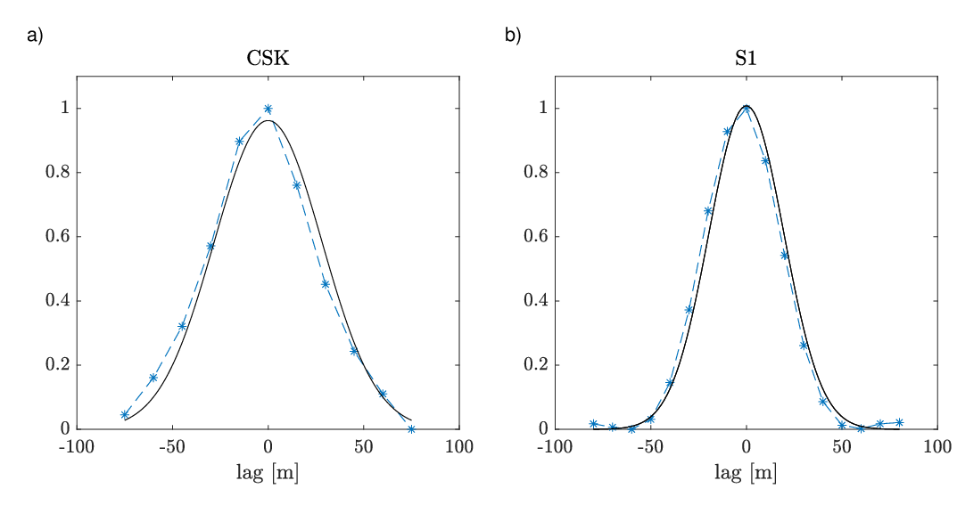
SAR observations play a crucial role in the present analysis as they provide estimates of the correlation length of the ice field. Indeed, SAR images are generally two-dimensional maps of the Earth surface, which supply a description of the different targets in the scene with details imposed by the geometric resolution of the imaging sensor. The signal backscattered by the surface carries primary information on both the roughness of the surface at the scale of the impinging electromagnetic radiation and the dielectric properties of the imaged target as well Franceschetti and Lanari 2018. As sea ice and water have well distinct roughness and dielectric properties Fu and Holt 1982, SAR sensors can provide a synoptic view of the field composition Toyota, Haas, and Tamura 2011.

Although for the MIZ a direct relation between the SAR signal and ice properties has not been established yet, there is evidence of a correlation between ice thickness, surface roughness and the radar cross-section (i.e the SAR signal) Toyota et al. 2011. Information on the correlation structure of the fluctuations in the ice cover can therefore be obtained through the analysis of the correlation function of the radar cross-section. A robust technique to estimate the correlation function from SAR is based on evaluating the inverse fast Fourier transform (IFFT) of the power spectral density (PSD) computed from the two-dimensional radar cross section Bendat and Piersol 2011. In order to remove the contribution of speckle noise at lag 0, a Butterworth filter is applied to the PSD before performing the IFFT Goldfinger 1982; De Carolis, Olla, and De Santi 2021.

We focus on observations on the 1st of November because of the availability of two SAR images acquired two hours apart over the area where the array of wave buoys was in operation. The first acquisition is performed by the X-band (9.6 GHz) SAR system on-board satellite number 3 of the Cosmo-SkyMed (CSK) constellation at 15:46 UTC; the second one by the C-band (9.6 GHz) SAR operated by the Sentinel-1A (S1) belonging to the Copernicus mission at 17:20 UTC. The two SAR acquisitions are shown together with the location of the wave buoys in Fig. 4 and reveal a MIZ composed of grease, pancake, and small ice floes.

For the blue-highligthed regions shown in Fig. 4, the SAR spectral analysis is performed to determine the correlation functions along the directions of the waves coming from the open ocean ( $\approx 224^{o}$ N) Stoica, Moses et al. 2005. As shown in Fig. 5, they are well fitted by Gaussian distributions of width $\lambda=26.83\,{\rm m}$ and $\lambda=19.52\,{\rm m}$ for the CSK and S1 acquisitions, respectively. It is worth noting that although the incoming dominant waves induce a quasi-periodic modulation of the microwave signal about 110 m long, the inferred $\lambda$ is well separated from this wavelength.

As shown in Fig. 4, buoy WB02 lies farthest inside the MIZ and is therefore taken as downstream reference buoy. However, none of the buoy pairs is aligned with the dominant wave direction (cyan arrow). The dotted lines identify the wavefronts at the location of the buoys; their distance to buoy WB02 defines the optical path along which wave attenuation is going to be evaluated. The sea ice properties in the transect between the wavefronts of the upstream buoys and buoy WB02 (blue region in Fig. 4) determines the measured wave attenuation.

Let us make the hypothesis that wave diffusion is the only attenuation mechanism for the incident waves. We can then use the value of $\lambda$ from analysis of the SAR images to carry out a best-fit of the buoy data on wave attenuation with Eqs. (57) and (48), to retrieve the values of the remaining parameters $\varphi_{inc}$ and $\overline{\tilde{h}^{2}}$ :

\displaystyle\min_{\overline{\tilde{h}^{2}},\varphi_{inc}}\sum_{i}\left[q_{m}({\bf k}_{i})-q_{eff}({\bf k}_{i};\overline{\tilde{h}^{2}},\varphi_{inc},\lambda)\right]^{2},

(63)

where $q_{m}$ are the measured data, obtained as described in Cheng et al. (2017)Cheng et al. 2017, and reanalyzed to clear the data from any unwanted instrumental noise energy Thomson et al. 2020. The procedure is detailed in the Appendix. We continue to assume $r_{2}=1$ in Eq. (48).

Best-fit samples of wave attenuation for measures close to the SAR acquisitions are reported in Fig. 6. Red circles represent the wave-buoy attenuation rates $q_{m}$ . Black lines show attenuation rates computed with Eqs. (48,57). The top panels show the attenuation rates measured at 15:30 UTC, and thus related to the CSK acquisition, while the bottom panels show the attenuation rates measured at 17:00 UTC and 17:30 UTC, and are related to the S1 acquisition.

In all cases, the fitting procedure can reproduce the structure of the rollover peak. We find in particular good agreement between the values of $\varphi_{inc}$ estimated by the fitting procedure and the ones from analysis of the angular spectrum from buoy data (see Fig. 7).

The inferred values for the variance, $\overline{\tilde{h}^{2}}=0.04-0.12\,\rm{m}^{2}$ , instead, are large compared to the expected values of the sea-ice thickness $h\approx 0.1\,{\rm m}$ at 16:54 UTC and $h\approx 0.15\,{\rm m}$ at 18:00 UTC, reported in the region of interest by the Arctic Shipborne Sea Ice Standardization Tool (ASSIST) Climate and Cryosphere Arctic Sea Ice Working Group () CliC-ASIWG. At the present stage, it is not clear whether the difficulty could be solved by a redefinition of $h$ and $r_{2}$ , or is a signal of actual smallness of the diffusion contribution to wave attenuation.

As shown in Fig. 7, the inferred $\varphi_{inc}$ well separates the dominant wave from another wave packet coming further from the west. The amplitude of the second wave packet increases with time, while the energy and the opening angle of the dominant wave decrease with time. It is worth noting that the directional spectra measured at the same time by different upstream buoys show significant differences, despite the buoys locations being sufficiently tight (see Fig. 4). The temporal evolution of the directional spectra of WB02 (red curves in Fig. 4), in particular, is difficult to interpret, with the peak wave energy at 17:00 UTC higher than the one of the other time stamps and the one of the upstream buoy.

IX Conclusion

We have studied the diffusion of gravity waves generated in a pancake-ice covered inviscid water column, with special focus on the role of random spatial variations in the thickness and the concentration of the ice layer. We have modeled pancake-ice as a horizontally inextensible, but otherwise stress-free continuum. At the scale of the individual ice body, the dynamics is realized most simply by assuming that the bodies are in close contact without the possibility of rafting.

Two mechanisms in the generation of wave radiation can be identified: vertical motions of the bodies, which generate radial waves, and horizontal motions of the bodies, which generate a dipole field with lobes along the direction of propagation of the incident wave (both motions defined relative to the unperturbed wave field). The contribution from higher order multipoles appears to be negligible for bodies much smaller than a wavelength. The dipole radiation is itself negligible if instead of a layer composed of many ice bodies, we have a continuous ice slab with an immersed surface of vanishing roughness.

We have evaluated the contribution to wave attenuation from diffusion in terms of the fraction of the diffused energy that is radiated at angles exceeding the opening angle $\varphi_{inc}$ of the incident wave.

We have found that wave diffusion is stronger for waves with wavelength comparable to the correlation length $\lambda$ of the fluctuations in the ice layer. The phenomenon is associated with a contribution to wave attenuation which is itself maximum near $\lambda$ , thus providing a mechanism for rollover similar to the one described in Wadhams (1986)Wadhams 1986, where the role of the parameter $\lambda$ was played by the radius of the individual floes. For $\lambda$ close to the observed rollover peak, it is indeed possible, with reasonable values of the amplitude of the fluctuations in the ice thickness and concentration, to generate an attenuation of the incident waves comparable to what is observed in field experiments. One may expect that similar phenomena could play a role in wave energy harvesting by large assemblies of wave energy converters Tokić and Yue 2021. The contribution to diffusion from the discreteness of the ice bodies, instead, is negligible for bodies much smaller than a wavelength and is further reduced if the mutual interaction of the bodies is not taken into account.

We have compared the results of the theory with buoy data from the Sikuliaq campaign in Autumn 2015 in the Arctic Thomson et al. 2018, and SAR images available in that region in the same period De Carolis, Olla, and De Santi 2021. We have followed the approach in Thomson et al. (2020)Thomson et al. 2020 to eliminate spurious instrumental noise contributions to the development of a rollover peak, and we have found that rollover persists in all analyzed data. We have found that the roughness map of the SAR images are characterized by spatial fluctuations peaked in the rollover region, which furnishes indirect evidence to possible inhomogeneity of the ice cover at that scale.

We have carried out a best-fit analysis of the attenuation data with the inferred value of $\lambda$ , in the assumption that wave diffusion is the only mechanism at play. The resulting fluctuation levels of $h$ are somewhat large, but not to the point of dismissing the possibility of an important role of diffusion in the attenuation process. A more definite statement would require going beyond the qualitative description of the layer structure afforded in Sec. VI.

Attenuation by diffusion could also explain the puzzling observation that fitting experimental data by viscous models requires an effective viscosity dependent on the ice thickness. As illustrated in Sec. VII, we see in fact that the small wavenumber scaling of the attenuation obtained by a diffusion-based model can be reproduced by viscous models such as the one by Keller and the CP model only by assuming an effective viscosity $\nu$ linearly proportional to the ice thickness De Carolis, Olla, and De Santi 2021.

The analysis in this paper is based on rough modeling assumptions on the dynamics of the ice layer, which are not too different from those at the basis of the mass-loading model Peters 1950; Keller and Weitz 1953; Wadhams 1986. The average wave dynamics obtained in the present theory coincides in fact with what would be obtained using a mass-loading model. An obvious question is whether the inextensibility hypothesis adopted in the present paper would still hold if the ice bodies in the layer interacted hydrodynamically rather than by contact forces. A numerical study of the matter is underway, following the approach detailed in Kagemoto and Yue 1986 and followed more recently in Meylan et al. 2021.

Acknowledgements.

This work has been supported by the Italian Piano Nazionale Ricerche in Antartide, (project WAMIZ, grant PNRA18/_00109) and by the EU FP7 project ICE-ARC (grant agreement 603887). The present work is a contribution to the Year of Polar Prediction (YOPP), a flagship activity of the Polar Prediction Project (PPP), initiated by the World Weather Research Programme (WWRP) of the World Meteorological Organisation (WMO). We acknowledge the WMO WWRP for its role in coordinating this international research activity. The CSK product used in this work was delivered by ASI (Italian Space Agency) under the ASI licence to use ID 714 in the framework of COSMO–SkyMed Open Call for Science. The Sentinel–1A used in this work was freely delivered by ESA through the Copernicus Open Access Hub (https://scihub.copernicus.eu).

Appendix A Data analysis procedure

The spectral noise energy $E_{n}(k)$ is assumed to follow the power-law $k^{-2}$ in the spectral tail above the peak with equivalent noise height $H_{n}=0.1$ m. The attenuation rates, $q_{m}$ , can be estimated from the measured attenuation, $q_{b}$ , as follows:

q_{m}(k)=q_{b}(k)+\cfrac{1}{D}\left[\cfrac{1+E_{n}(k)/E_{D}(k)}{1+E_{n}(k)/E_{U}(k)}\right],

(64)

where $E_{U}$ and $E_{D}$ are the noise-free, omni-directional wave energy spectra of the upstream and the downstream buoy, respectively, and $D$ is the distance travelled by the waves between the couple of buoys. Note that the energy bias negligibly affected the attenuation rates $q_{m}$ , meaning that data processing performed by Cheng et al. 2017 already properly accounted for noise contamination.

References

Squire (1995) V. Squire, “Of ocean waves and ice sheets,” Annu. Rev. Fluid Mech. 27, 115–168 (1995).
Thomson and Rogers (2014) J. Thomson and W. E. Rogers, “Swell and sea in the emerging arctic ocean,” Geophysical Research Letters 41, 3136–3140 (2014).
Parkinson and Comiso (2013) C. L. Parkinson and J. C. Comiso, “On the 2012 record low arctic sea ice cover: Combined impact of preconditioning and an august storm,” Geophysical Research Letters 40, 1356–1361 (2013).
Thomson et al. (2018) J. Thomson, S. Ackley, F. Girard-Ardhuin, F. Ardhuin, A. Babanin, G. Boutin, J. Brozena, S. Cheng, C. Collins, M. Doble, et al., “Overview of the arctic sea state and boundary layer physics program,” Journal of Geophysical Research: Oceans 123, 8674–8687 (2018).
Squire (2007) V. A. Squire, “Of ocean waves and sea-ice revisited,” Cold Regions Science and Technology 49, 110–133 (2007).
Squire (2020) V. A. Squire, “Ocean wave interactions with sea ice: a reappraisal,” Annual Review of Fluid Mechanics 52, 37–60 (2020).
Wadhams et al. (1999) P. Wadhams, F. Parmiggiani, G. De Carolis, and M. Tadross, “Mapping the thickness of pancake ice using ocean wave dispersion in sar imagery,” in Oceanography of the Ross Sea Antarctica (Springer, 1999) pp. 17–34.
De Carolis (2001) G. De Carolis, “Retrieval of the ocean wave spectrum in open and thin ice covered ocean waters from ers synthetic aperture radar images,” Nuovo Cimento. C 24, 53–66 (2001).
Wadhams, Parmiggiani, and De Carolis (2002) P. Wadhams, F. Parmiggiani, and G. De Carolis, “The use of sar to measure ocean wave dispersion in frazil–pancake icefields,” Journal of physical oceanography 32, 1721–1746 (2002).
De Carolis (2003) G. De Carolis, “Sar measurements of directional wave spectra in viscous sea ice,” Rivista Italiana di TELERILEVAMENTO 26, 31–36 (2003).
Wadhams et al. (2004) P. Wadhams, F. Parmiggiani, G. De Carolis, D. Desiderio, and M. Doble, “Sar imaging of wave dispersion in antarctic pancake ice and its use in measuring ice thickness,” Geophysical Research Letters 31 (2004).
Sutherland and Gascard (2016) P. Sutherland and J.-C. Gascard, “Airborne remote sensing of ocean wave directional wavenumber spectra in the marginal ice zone,” Geophysical Research Letters 43, 5151–5159 (2016).
Wadhams et al. (2018) P. Wadhams, G. Aulicino, F. Parmiggiani, P. Persson, and B. Holt, “Pancake ice thickness mapping in the beaufort sea from wave dispersion observed in sar imagery,” Journal of Geophysical Research: Oceans 123, 2213–2237 (2018).
De Carolis, Olla, and De Santi (2021) G. De Carolis, P. Olla, and F. De Santi, “Sar image wave spectra to retrieve the thickness of grease-pancake sea ice using viscous wave propagation models,” Scientific Reports 11, 1–14 (2021).
Masson and LeBlond (1989) D. Masson and P. LeBlond, “Spectral evolution of wind-generated surface gravity waves in a dispersed ice field,” Journal of Fluid Mechanics 202, 43–81 (1989).
Bennetts and Squire (2012) L. G. Bennetts and V. A. Squire, “On the calculation of an attenuation coefficient for transects of ice-covered ocean,” Proceedings of the Royal Society A: Mathematical, Physical and Engineering Sciences 468, 136–162 (2012).
Meylan and Squire (1996) M. H. Meylan and V. A. Squire, “Response of a circular ice floe to ocean waves,” Journal of Geophysical Research: Oceans 101, 8869–8884 (1996).
Meylan et al. (2015) M. Meylan, L. Bennetts, C. Cavaliere, A. Alberello, and A. Toffoli, “Experimental and theoretical models of wave-induced flexure of a sea ice floe,” Physics of Fluids 27, 041704 (2015).
Li, Shi, and Wu (2021) Z. Li, Y. Shi, and G. Wu, “Interaction of ocean wave with a harbor covered by an ice sheet,” Physics of Fluids 33, 057109 (2021).
Kohout and Meylan (2008) A. L. Kohout and M. H. Meylan, “An elastic plate model for wave attenuation and ice floe breaking in the marginal ice zone,” Journal of Geophysical Research: Oceans 113 (2008).
Squire and Montiel (2016) V. A. Squire and F. Montiel, “Evolution of directional wave spectra in the marginal ice zone: a new model tested with legacy data,” Journal of Physical Oceanography 46, 3121–3137 (2016).
Toyota, Haas, and Tamura (2011) T. Toyota, C. Haas, and T. Tamura, “Size distribution and shape properties of relatively small sea-ice floes in the antarctic marginal ice zone in late winter,” Deep Sea Research Part II: Topical Studies in Oceanography 58, 1182–1193 (2011).
Doble, Coon, and Wadhams (2003) M. J. Doble, M. D. Coon, and P. Wadhams, “Pancake ice formation in the weddell sea,” Journal of Geophysical Research: Oceans 108 (2003).
Doble et al. (2015) M. J. Doble, G. De Carolis, M. H. Meylan, J.-R. Bidlot, and P. Wadhams, “Relating wave attenuation to pancake ice thickness, using field measurements and model results,” Geophysical Research Letters 42, 4473–4481 (2015).
Keller (1998) J. B. Keller, “Gravity waves on ice-covered water,” Journal of Geophysical Research: Oceans 103, 7663–7669 (1998).
Wang and Shen (2010) R. Wang and H. H. Shen, “Gravity waves propagating into an ice-covered ocean: A viscoelastic model,” Journal of Geophysical Research: Oceans 115 (2010).
Chen, Gilbert, and Guyenne (2019) H. Chen, R. P. Gilbert, and P. Guyenne, “Dispersion and attenuation in a porous viscoelastic model for gravity waves on an ice-covered ocean,” European Journal of Mechanics-B/Fluids 78, 88–105 (2019).
De Carolis and Desiderio (2002) G. De Carolis and D. Desiderio, “Dispersion and attenuation of gravity waves in ice: a two-layer viscous fluid model with experimental data validation,” Physics Letters A 305, 399–412 (2002).
De Santi and Olla (2017) F. De Santi and P. Olla, “Effect of small floating disks on the propagation of gravity waves,” Fluid Dynamics Research 49, 025512 (2017).
Cheng et al. (2017) S. Cheng, W. E. Rogers, J. Thomson, M. Smith, M. J. Doble, P. Wadhams, A. L. Kohout, B. Lund, O. P. Persson, C. O. Collins, et al., “Calibrating a viscoelastic sea ice model for wave propagation in the arctic fall marginal ice zone,” Journal of Geophysical Research: Oceans 122, 8770–8793 (2017).
De Santi et al. (2018) F. De Santi, G. De Carolis, P. Olla, M. Doble, S. Cheng, H. H. Shen, P. Wadhams, and J. Thomson, “On the ocean wave attenuation rate in grease-pancake ice, a comparison of viscous layer propagation models with field data,” Journal of Geophysical Research: Oceans 123, 5933–5948 (2018).
Sutherland et al. (2019) G. Sutherland, J. Rabault, K. H. Christensen, and A. Jensen, “A two layer model for wave dissipation in sea ice,” Applied Ocean Research 88, 111–118 (2019).
Li et al. (2017) J. Li, A. L. Kohout, M. J. Doble, P. Wadhams, C. Guan, and H. H. Shen, “Rollover of apparent wave attenuation in ice covered seas,” Journal of Geophysical Research: Oceans 122, 8557–8566 (2017).
Thomson et al. (2020) J. Thomson, L. Hovseková, M. H. Meylan, A. L. Kohout, and N. Kumar, “Spurious rollover of wave attenuation rates in sea ice caused by noise in field measurements,” Journal of Geophysical Research: Oceans , e2020JC016606 (2020).
Polnikov and Lavrenov (2007) V. Polnikov and I. Lavrenov, “Calculation of the nonlinear energy transfer through the wave spectrum at the sea surface covered with broken ice,” Oceanology 47, 334–343 (2007).
Liu and Mollo-Christensen (1988) A. K. Liu and E. Mollo-Christensen, “Wave propagation in a solid ice pack,” Journal of physical oceanography 18, 1702–1712 (1988).
Perrie and Hu (1996) W. Perrie and Y. Hu, “Air–ice–ocean momentum exchange. part 1: Energy transfer between waves and ice floes,” Journal of physical oceanography 26, 1705–1720 (1996).
Shen and Squire (1998) H. H. Shen and V. A. Squire, “Wave damping in compact pancake ice fields due to interactions between pancakes,” Antarctic Sea Ice: Physical Processes, Interactions and Variability 74, 325–341 (1998).
Skene et al. (2015) D. Skene, L. Bennetts, M. Meylan, and A. Toffoli, “Modelling water wave overwash of a thin floating plate,” (2015).
Kagemoto and Yue (1986) H. Kagemoto and D. K. Yue, “Interactions among multiple three-dimensional bodies in water waves: an exact algebraic method,” Journal of fluid mechanics 166, 189–209 (1986).
Peters (1950) A. S. Peters, “The effect of a floating mat on water waves,” Commun. Pure Appl. Math. 3, 319–354 (1950).
Keller and Weitz (1953) J. B. Keller and M. Weitz, “Reflection and transmission coefficients for waves entering or leaving an icefield,” Commun. Pure Appl. Math. 6, 415–417 (1953).
Peter and Meylan (2004a) M. A. Peter and M. H. Meylan, “The eigenfunction expansion of the infinite depth free surface green function in three dimensions,” Wave Motion 40, 1–11 (2004a).
Landau and Lifshitz (1987) L. D. Landau and E. M. Lifshitz, Fluid Mechanics, Vol. 6 (Pergamon Press, 1987).
Jackson (1999) J. D. Jackson, “Classical electrodynamics,” (1999).
Abramowitz, Stegun, and Romer (1988) M. Abramowitz, I. A. Stegun, and R. H. Romer, “Handbook of mathematical functions with formulas, graphs, and mathematical tables,” (1988).
Landau and Lifshitz (2013) L. D. Landau and E. M. Lifshitz, Quantum mechanics: non-relativistic theory, Vol. 3 (Elsevier, 2013).
Peter and Meylan (2004b) M. A. Peter and M. H. Meylan, “Infinite-depth interaction theory for arbitrary floating bodies applied to wave forcing of ice floes,” (2004b).
Howe (1971) M. Howe, “Wave propagation in random media,” Journal of Fluid Mechanics 45, 769–783 (1971).
Sternberg (1995) S. Sternberg, Group theory and physics (Cambridge University Press, 1995).
Montiel, Squire, and Bennetts (2016) F. Montiel, V. Squire, and L. Bennetts, “Attenuation and directional spreading of ocean wave spectra in the marginal ice zone,” Journal of Fluid Mechanics 790, 492–522 (2016).
Wadhams (1986) P. Wadhams, “The seasonal ice zone,” in The geophysics of sea ice (Springer, 1986) pp. 825–991.
Meylan et al. (2021) M. H. Meylan, C. Horvat, C. M. Bitz, and L. G. Bennetts, “A floe size dependent scattering model in two-and three-dimensions for wave attenuation by ice floes,” Ocean Modelling 161, 101779 (2021).
Marquart et al. (2021) R. Marquart, A. Bogaers, S. Skatulla, A. Alberello, A. Toffoli, C. Schwarz, and M. Vichi, “A computational fluid dynamics model for the small-scale dynamics of wave, ice floe and interstitial grease ice interaction,” Fluids 6, 176 (2021).
Newyear and Martin (1999) K. Newyear and S. Martin, “Comparison of laboratory data with a viscous two-layer model of wave propagation in grease ice,” Journal of Geophysical Research: Oceans 104, 7837–7840 (1999).
Climate and Cryosphere Arctic Sea Ice Working Group () (CliC-ASIWG) Climate and Cryosphere Arctic Sea Ice Working Group (CliC-ASIWG), “Arctic shipborne sea ice standardization tool,” [Online; accessed 15-March-2021].
Franceschetti and Lanari (2018) G. Franceschetti and R. Lanari, Synthetic aperture radar processing (CRC press, 2018).
Fu and Holt (1982) L.-L. Fu and B. Holt, Seasat views oceans and sea ice with synthetic-aperture radar, Vol. 81 (California Institute of Technology, Jet Propulsion Laboratory, 1982).
Toyota et al. (2011) T. Toyota, S. Ono, K. Cho, and K. I. Ohshima, “Retrieval of sea-ice thickness distribution in the sea of okhotsk from alos/palsar backscatter data,” Annals of glaciology 52, 177–184 (2011).
Bendat and Piersol (2011) J. S. Bendat and A. G. Piersol, “Random data: analysis and measurement procedures, vol. 729,” Hoboken, NJ: John Wiley & Sons (2011).
Goldfinger (1982) A. D. Goldfinger, “Estimation of spectra from speckled images,” IEEE transactions on aerospace and electronic systems , 675–681 (1982).
Stoica, Moses et al. (2005) P. Stoica, R. L. Moses, et al., “Spectral analysis of signals,” (2005).
Tokić and Yue (2021) G. Tokić and D. K. Yue, “Hydrodynamics of large wave energy converter arrays with random configuration variations,” Journal of Fluid Mechanics 923 (2021).

Diffusion of gravity waves by random space inhomogeneities in pancake-ice fields. Theory and validation with wave buoys and SARPreprint: AIP/123-QED