Implementation of a $3\times 3$ directionally-unbiased linear optical multiport

Quantum walks (QW), the quantum analogue of classical random walks, provide promising methodologies to execute complex quantum algorithms for quantum computing Kempe2003; Venegas2012. As random walks are used for algorithm design in classical computer, many quantum algorithms are developed based on QW which provide speed-up over the best known classical algorithms for the same problem Childs2002. Furthermore, this approach has capability of performing algorithms for universal quantum computation Crespi2013; Simon2018; Childs2009; Aharonov1993; Aharonov2001. Linear optics has been considered as one of the most promising candidates for implementing QW, because of its robustness against decoherence, ease of preparation of quantum states and its scalability through on-chip integration Carolan2015; Carolan2014; Tillmann2013; Tang2018.

QW are movements of walkers on a graph, which consist of connected vertices with N edges Tang2018_2; Faccin2013; Tregenna2003; Bian2017. A walker moves from a vertex to one of the neighboring vertices at each step. In linear optics, each vertex can be implemented by an $\textit{N}\times\textit{N}$ multiport which is a linear optical element having N input ports and $N$ output ports. A set of phase shifters and $2\times 2$ beam splitters (BSs) can construct an $N\times N$ multiport with $N\geq 3$ Reck1994; Clements2016. Since directionality of a BS forbids input photons to move back to the same port where the input photons entered, an implementation of an $N\times N$ multiport forms a unidirectional expending tree-like structure to cover all possible optical paths. From the inability of reverse propagation, this unidirectional implementation is called a directionally-biased multiport.

Recently, a directionally-unbiased multiport has been proposed Simon2016. Unlike a directionally-biased multiport, it allows an input photon to leave the same port where the input photon entered. Hence, it is suitable for implementing undirected graphs for QW. The bidirectional feature of the directionally-unbiased multiports can surprisingly reduce the resource requirement for some QW configurations Simon2016.

It has been reported only an experimental implementation of an $N\times N$ directionally-unbiased multiport for $N\geq 3$ Osawa2018. Osawa et al. implemented a $3\times 3$ directionally-unbiased multiport based on an optical cavity in free space using bulk optical elements Osawa2018. However, this scheme requires input photons having a long coherence length due to large path length differences among the different trajectories in the cavity. Indeed, it was experimentally tested with a HeNe laser beam whose coherence length is longer than 1 km. It does not show the quantum optical phenemoena in directionally-unbiased multiports, and yet there has been no experimental demonstration of directionally-unbiased multiport using quantum linght sources.

In this paper, we experimentally demonstrate a $3\times 3$ directionally-unbiased linear optical multiport using a $3\times 3$ optical fiber BS, or a tritter. By measuring the two-photon Hong-Ou-Mandel (HOM) interference Hong1987 and amplitude distribution ratios of the $3\times 3$ directionally-unbiased multiport, we reconstructed a transfer matrix of the implemented multiport. All results are obtained using quantum light sources. We believe that our directionally-unbiased multiport device can be useful building blocks for simulating QWs on complex graph networks.

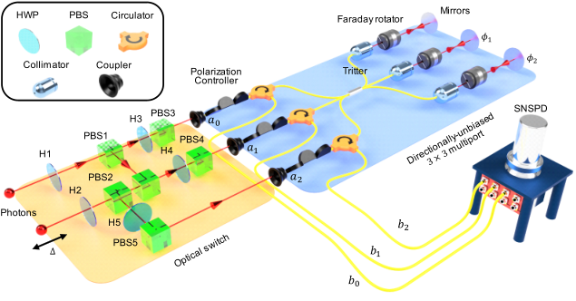
The schematic of our experimental setup to implement and analyze a $3\times 3$ directionally-unbiased optical fiber multiport is shown in Fig. 2. We generate a pair of identical single photons with the center wavelength of 1556 nm via type-II spontaneous parametric down conversion (SPDC) process using a 10 mm-thick PPKTP crystal (poling period of 46.15 $\mu$m) pumped by femtosecond laser pulses (not shown in Fig. 2). The power and repetition rate of the pump are 10 mW and 125 MHz, respectively. The indistinguishability between photons is verified by the HOM interference visibility of $\mathcal{V}\sim 0.99$ Lee2021. Note that the coherence length of our down-converted photons is $\sim 440\mu$m, which is much narrower than the coherence length of a He-Ne laser.

By using a set of waveplates and polarizing beam splitters (PBSs), we can prepare the input state $\hat{a}^{\dagger}_{i}\hat{a}^{\dagger}_{j}|0\rangle$ and $\hat{a}^{\dagger}_{i}|0\rangle$ with horizontal polarization where $i,j=0,1,2~(i\neq j)$ for measuring visibility of the two-photon HOM interference and amplitude distributions, respectively. In order to choose the combination of the input ports, we adjust the polarization of the input photons using a set of half waveplates (Hs) as shown in the optical switch of Fig. 2. For example, $\hat{a}^{\dagger}_{0}\hat{a}^{\dagger}_{1}|0\rangle$ input state can be prepared by setting the angles of (H1, H2, H3, H4, H5) as (0^∘, 0^∘, 0^∘, 0^∘, 45^∘). Additionally, we can obtain either $\hat{a}^{\dagger}_{0}|0\rangle$ or $\hat{a}^{\dagger}_{1}|0\rangle$ input state by setting the angles of (H3, H4) as either (0^∘, 45^∘) or (45^∘, 0^∘), respectively. Using this method, we can send all combinations of single and two-photon input states into our $3\times 3$ multiport.

Note that photons at each input mode should have the same polarization for indistinguishability between two photons. We can adjust the polarization of the photons inside a tritter using fiber polarization controllers. Moreover, Faraday rotators located between the output mode of a tritter and a mirror guarantee that photons propagating in the opposite directions do not interfere with each other. We can isolate the photons coming out from the input ports using optical fiber circulators, and send them toward superconducting nanowire single photon detectors (SNSPDs) for single photon detection. Single photon count rates for $\hat{b}^{\dagger}_{k}|0\rangle$ with input states $\hat{a}^{\dagger}_{i}|0\rangle$ are obtained for measuring amplitude distribution ratios, and all possible combinations of the two-photon coincidence detection events $\hat{b}^{\dagger}_{k}\hat{b}^{\dagger}_{l}|0\rangle$ where $k,l=0,1,2~(k\neq l)$ with input states $\hat{a}^{\dagger}_{i}\hat{a}^{\dagger}_{j}|0\rangle~(i\neq j)$ for measuring the two-photon HOM interference are obtained using a home-made coincidence counting unit (CCU) Park2015; Park2021.

For measuring visibilities of the two-photon HOM interference, we introduced an optical delay $\Delta$ between two input photons by scanning the position of one collimator using a motorized linear stage. We measure all possible combinations of the two-photon HOM interference fringe for each input state $\hat{a}^{\dagger}_{i}\hat{a}^{\dagger}_{j}|0\rangle$. In order to obtain amplitude distribution ratios of the multiport, all possible single photon count rates $n_{ki}$ are measured for each input state $\hat{a}^{\dagger}_{i}|0\rangle$. The position of the motorized linear stage is rearranged whenever the input state is changed, to set an optical delay $\Delta=0$.

Here, we experimentally reconstruct a transfer matrix of our implemented directionally-unbiased multiport devices as shown in Fig. 2 using two independent reconstruction methods. First, we directly reconstruct a transfer matrix $V$ as Eq. (5) by minimizing Eq. (10). Second, we reconstruct the transfer matrix $W=U_{B}\varPhi U_{F}$ as Eq. (4), and by independently reconstructing $U_{F}$ and $U_{B}$, and $\varPhi$. Then, we compare two reconstructed transfer matrices $V$ and $W$.

We first experimentally reconstruct the optimal transfer matrix $V$ of our $3\times 3$ directionally-unbiased multiport using the measured HOM visibility matrix $\mathcal{V}_{M}$ and the amplitude distribution $|u_{ki}|^{2}$. All possible combinations of the HOM interferences are measured, and experimental results and corresponding fitting functions are shown in Fig. 3. From the experimental results, $\mathcal{V}_{M}$ is obtained to be

where the rows x and columns y of the matrix $\mathcal{V}_{M}$ correspond to the input state $x=\{\hat{a}^{\dagger}_{0}\hat{a}^{\dagger}_{1}|0\rangle,\hat{a}^{\dagger}_{0}\hat{a}^{\dagger}_{2}|0\rangle,\hat{a}^{\dagger}_{1}\hat{a}^{\dagger}_{2}|0\rangle\}$ and the output detection basis $y=\{\hat{b}^{\dagger}_{0}\hat{b}^{\dagger}_{1}|0\rangle,\hat{b}^{\dagger}_{0}\hat{b}^{\dagger}_{2}|0\rangle,\hat{b}^{\dagger}_{1}\hat{b}^{\dagger}_{2}|0\rangle\}$, respectively.

From the measured count rate, the amplitude distribution $|u_{M}|^{2}$ is obtained by using Eq. (6). The matrix of the amplitude distribution $|u_{M}|^{2}$ is obtained to be

From the measurement results $\mathcal{V}_{M}$ and $|u_{M}|^{2}$, we numerically found a transfer matrix $V$ of our implemented directionally-unbiased $3\times 3$ linear optical multiport. The experimentally reconstructed matrix $V$ and the corresponding standard deviation $\sigma_{V}$ are given by

and

respectively. The reconstructed matrix $V$ is shown in Fig. 4(a). The obtained similarity in Eq. (11) between $\mathcal{V}_{M}$ and $\mathcal{V}_{V}$ is $S_{MV}=0.937\pm 0.003$, which demonstrates that $V$ describes our directionally-unbiased $3\times 3$ linear optical multiport well.

In order to confirm that our implemented multiport is a directionally-unbiased $3\times 3$, we independently reconstruct a transfer matrix $W=U_{B}\varPhi U_{F}$. To obtain $W$, we independently reconstruct $U_{F}$ and $U_{B}$ by measuring the HOM visibility matrix and the amplitude distribution, respectively. We performed this measurement by removing mirror units and connecting the outputs of the tritter into the SNSPDs. The obtained HOM visibility matrix and the amplitude distribution data are presented in Appendix A. With these data, the experimentally reconstructed $U_{F}$ and the corresponding standard deviation $\sigma_{F}$ are

and

respectively. Likewise, the experimentally reconstructed $U_{B}$ and the corresponding standard deviation $\sigma_{B}$ are given by

and

respectively.

By substituting reconstructed $U_{F}$ and $U_{B}$ to Eq. (4), we numerically obtain the $\varPhi$ by minimizing the $RMS2=\Sigma(\mathcal{V}_{W}-\mathcal{V}_{M})^{2}$ by varying the $\phi_{1}$ and $\phi_{2}$, here $\mathcal{V}_{W}$ denotes the calculated visibility matrix from $W$. By combining the obtained phase parameters $[\phi_{1},\phi_{2}]=[(0.383\pm 0.014)\pi,(-0.596\pm 0.010)\pi]$ and the transfer matrices $U_{B}$ and $U_{F}$, we obtain the transfer matrix of the implemented $3\times 3$ directionally-unbiased multiport $W_{0}$. Then, we can obtain the corresponding equivalent real-bordered matrix $W$ and standard deviation, which are given by

and

respectively, where the real-bordered matrix denotes the matrix form described on Eq. (5). The detailed information on how we obtain the real-bordered matrix is provided in Appendix B. The similarity between $\mathcal{V}_{M}$ and $\mathcal{V}_{W}$ is $S_{MW}=0.972\pm 0.007$ and $W$ is graphically shown in Fig. 4(b).

In order to compare the reconstructed transfer matrices $V$ and $W$, we use fidelity $F$ between two matrices, which is defined by Polino2019

where $0\leq F\leq 1$. High fidelity means matrices are similar with each other. The obtained fidelity is $F(V,W)=0.971\pm 0.005$, meaning that these two transfer matrices are highly similar to each other and verifies Eq. (4).

We experimentally demonstrated a $3\times 3$ directionally-unbiased linear optical multiport consisting of a tritter and mirrors. We reconstructed the transfer matrix from the experimental two-photon HOM visibility and amplitude distributions via two independent reconstruction methods, and confirmed that two methods give the similar results in terms of the fidelity. Comparing to the previous demonstration of a $3\times 3$ directionally-unbiased multiport based on bulk optics elements Osawa2018, our $3\times 3$ directionally-unbiased linear optical multiport does not require a long coherence length of the light source. We also note that our experiment is the first demonstration of quantum optical phenomenon using $3\times 3$ directionally-unbiased multiport. We emphasize that our scheme can be easily extended to implement a $N\times N$ directionally-unbiased linear optical multiport by replacing a tritter into a $N\times N$ multiport BS.

Since a directionally-unbiased multiport can be a single vertex having multiple edges in a graph, we can perform QW simulation on a complex graph networks by combining a number of directionally-unbiased multiports. For example, our $3\times 3$ directionally-unbiased multiport can construct a hexagonal lattice. Complex graph networks composed of directionally-unbiased multiports can also be used for simulating various Hamiltonians and topological physics Simon2017; Simon2017_2; Simon2020; Simon2018. Moreover, our directionally-unbiased multiport can be imprinted on an integrated photonic circuits Peruzzo2011 so that the phases of the multiport can be even more stabilized and the relative phases can be tunable electrically. We believe that our results can provide a practical platform to perform quantum simulations on complex graph networks.

This work was supported by the National Research Foundation of Korea (NRF) (2019M3E4A1079777, 2019M3E4A1078660, 2021R1C1C1003625), the Institute for Information and Communications Technology Promotion (IITP) (2020-0-00947, 2020-0-00972), and the KIST research program (2E31021).

References

- (1) J. Kempe, Quantum random walks: an introductory overview, Contemp. Phys. 44, 307–327 (2003).
- (2) S. E. Venegas-Andraca, Quantum walks: a comprehensive review, Quantum Inf. Process. 11, 1015–1106 (2012).
- (3) A. M. Childs, E. Farhi, and S. Gutmann, An example of the difference between quantum and classical random walks, Quantum Inf. Process. 1, 35–43 (2002).
- (4) A. Crespi, R. Osellame, R. Ramponi, D. J. Brod, E. F. Galvão, N. Spagnolo, C. Vitelli, E. Maiorino, P. Mataloni, and F. Sciarrino, Integrated multimode interferometers with arbitrary designs for photonic boson sampling, Nat. Photonics 7, 545–549 (2013).
- (5) D. S. Simon, S. Osawa, and A. V. Sergienko, Joint entanglement of topology and polarization enables error protected quantum registers, New J. Phys. 20, 093032 (2018).
- (6) A. M. Childs, Universal computation by quantum walk, Phys. Rev. Lett. 102, 180501 (2009).
- (7) Y. Aharonov, L. Davidovich, and N. Zagury, Quantum random walks, Phys. Rev. A 48, 1687–1690 (1993).
- (8) D. Aharonov, A. Ambainis, J. Kempe, and U. Vazirani, Quantum walks on graphs, in Proceedings of the 33rd annual ACM symposium on theory of computing (ACM,2001), pp. 50–59.
- (9) J. Carolan, C. Harrold, C. Sparrow, E. Martin-López, N. J. Russell, J. W. Silverstone, P. J. Shadbolt, N. Matsuda, M. Oguma, M. Itoh, G. D. Marshall, M. G. Thompson, J. C.F. Mattews, T. Hashimoto, J. L. O’Brien, and A. Laing, Universal linear optics, Science 349, 711–716 (2015).
- (10) J. Carolan, J. D. A. Meinecke, P. J. Shadbolt, N. J. Russell, N. Ismail, K. Wörhoff, T. Rudolph, M. G. Thompson, J. L. O’Brien, J. C. F. Matthews, and A. Laing, On the experimental verification of quantum complexity in linear optics, Nat. Photonics 8, 621–626 (2014).
- (11) M. Tillmann, B. Dakić, R. Heilmann, S. Nolte, A. Szameit, and P. Walther, Experimental boson sampling, Nat. Photonics 7, 540–544 (2013).
- (12) H. Tang, X. F. Lin, Z. Feng, J. Y. Chen, J. Gao, K. Sun, C. Y. Wang, P. C. Lai, X. Y. Xu, Y. Wang, L. F. Qiao, A. -L. Yang, and X. M. Jin, Experimental two-dimensional quantum walk on a photonic chip, Sci. Adv. 4, t3174 (2018).
- (13) H. Tang, C. D. Franco, Z. Y. Shi, T. S. He, Z. Feng, J. Gao, K. Sum, Z. M. Li, Z. Q. Jiao, T. Y. Wang, M. S. Kim, and X. M. Jin, Experimental quantum fast hitting on hexagonal graphs, Nat. Photonics 12, 754–758 (2018).
- (14) M. Faccin, T. Johnson, J. Biamonte, S. Kais, and P. Migdal, Degree Distribution in Quantum Walks on Complex Networks, Phys. Rev. X. 3, 041007 (2013).
- (15) B. Tregenna, W. Flanagan, R. Maile, and V. Kendon, Controlling discrete quantum walks: coins and initial states, New J. Phys. 5, 83 (2003).
- (16) Z. H. Bian, J. Li, X. Zhan, J. Twamley, and P. Xue, Experimental implementation of a quantum walk on a circle with single photons, Phys. Rev. A 95, 052338 (2017).
- (17) M. Reck, A. Zeilinger, H. J. Bernstein, and P. Bertani, Experimental realization of any discrete unitary operator, Phys. Rev. Lett. 73, 58–61 (1994).
- (18) W. R. Clements, P. C. Humphreys, B. J. Metcalf, W. S. Kolthammer, and I. A. Walmsley, An optimal design for universal multiport interferometers, Optica 3, 1460–1465 (2016).
- (19) D. S. Simon, C. A. Fitzpatrick, and A. V. Sergienko, Group transformations and entangled-sate quantum gates with directionally unbiased linear-optical multiports, Phys. Rev. A 93, 043845 (2016).
- (20) S. Osawa, D. S. Simon, and A. V. Sergienko, Experimental demonstration of a directionally-unbiased linear optical multiport, Opt. Express 26, 27201–27211 (2018).
- (21) C. K. Hong, Z. Y. Ou, and L. Mandel, Measurement of subpicosecond time intervals between two photons by interference, Phy. Rev. Lett. 59, 2044–2046 (1987).
- (22) S. Osawa, D. S. Simon, and A. V. Sergienko, Directionally-unbiased unitary optical devices in discrete-time quantum walks, Entropy 21, 853 (2019).
- (23) E. Peruzzo, A. Laing, A. Politi, T. Rudolph, and J. L. O’Brien, Multimode quantum interference of photons in multiport integrated devices, Nat. Commun. 2, 224 (2011).
- (24) N. Spagnolo, C. Vitelli, L. Aparo, P. Mataloni, F. Sciarrino, A. Crespi, R. Ramponi, and R. Osellame, Three-photon bosonic coalescence in an integrated tritter, Nat. Commun. 4, 1606 (2013).
- (25) D. Lee, Y. W. Cho, H. T. Lim, S. W. Han, H. Jung, S. Moon, and Y. S. Kim, Characterizing Bell state analyzer using weak coherent pulses, Quantum Inf. Process. 20, 149 (2021).
- (26) B. K. Park, Y. S. Kim, O. Kwon, S. W. Han, and S. Moon, High-performance reconfigurable coincidence counting unit based on a field programmable gate array, Appl. Opt. 54, 4727–4731 (2015).
- (27) B. K. Park, Y. S. Kim, Y. W. Cho, S. Moon, and S. W. Han, Arbitrary configurable 20-channel coincidence counting unit for multi-qubit quantum Eexperiment, Electronics 10, 569 (2021).
- (28) E. Polino, M. Riva, M. Valeri, R. Silvestri, G. Corrielli, A. Crespi, N. Spagnolo, R. Osellame, and F. Sciarrino, Experimental multiphase estimation on a chip, Optica 6, 288–295 (2019).
- (29) D. S. Simon, C. A. Fitzpatrick, S. Osawa, and A. V. Sergienko, Quantum simulation of discrete-time hamiltonians using directionally unbiased linear optical multiports, Phys. Rev. A 95, 042109 (2017).
- (30) D. S. Simon, C. A. Fitzpatrick, S. Osawa, and A. V. Sergienko, Quantum simulation of topologically protected states using directionally unbiased linear-optical multiports, Phys. Rev. A 96, 013858 (2017).
- (31) D. S. Simon, S. Osawa, and A. V. Sergienko, Quantum clustered two-photon walks, Phys. Rev. A 101, 032118 (2020).