2021
\trnumberCMU-ML-21-101
\committee
Ruslan Salakhutdinov, Chair
Abhinav Gupta
Deva Ramanan
Jitendra Malik
This research was supported by: Air Force Research Laboratory award FA875016C0130001, Defense Advanced Research Projects Agency award HR001116C0136, Department of the Interior award D17PC00340, National Science Foundation award IIS1216282, a graduate fellowship from Facebook, and a research grant from Apple. \disclaimer
Building Intelligent Autonomous Navigation Agents
Abstract
Breakthroughs in machine learning in the last decade have led to ‘digital intelligence’, i.e. machine learning models capable of learning from vast amounts of labeled data to perform several digital tasks such as speech recognition, face recognition, machine translation and so on. The goal of this thesis is to make progress towards designing algorithms capable of ‘physical intelligence’, i.e. building intelligent autonomous navigation agents capable of learning to perform complex navigation tasks in the physical world involving visual perception, natural language understanding, reasoning, planning, and sequential decision making. Despite several advances in classical navigation methods in the last few decades, current navigation agents struggle at long-term semantic navigation tasks. In the first part of the thesis, we discuss our work on short-term navigation using end-to-end reinforcement learning to tackle challenges such as obstacle avoidance, semantic perception, language grounding, and reasoning. In the second part, we present a new class of navigation methods based on modular learning and structured explicit map representations, which leverage the strengths of both classical and end-to-end learning methods, to tackle long-term navigation tasks. We show that these methods are able to effectively tackle challenges such as localization, mapping, long-term planning, exploration and learning semantic priors. These modular learning methods are capable of long-term spatial and semantic understanding and achieve state-of-the-art results on various navigation tasks.
keywords
Visual Navigation, Exploration, Deep Reinforcement LearningTo my wife and parents
Acknowledgements.
I am immensely grateful to my advisor, Ruslan Salakhutdinov. Russ is well-known for his knowledge and research experience. His guidance has been critical in shaping and directing this thesis. Russ also has many other remarkable qualities which made me realize how fortunate I am to be advised by him. He provided me complete intellectual freedom to pursue my research ideas, and yet every time I met with Russ, he was always as excited about my research as I was, if not more. Countless times, I have left his office feeling more inspired and motivated. He has provided me endless guidance and encouragement, and unconditional support for anything I have ever needed for my research. I am also extremely fortunate to work with Abhinav Gupta during the latter half of my Ph.D. Abhinav has an extraordinary ability to create a fun research environment that makes everyone around him feel comfortable in having honest and candid discussions with him about any topic. His sincere feedback has proved to be invaluable in not only research but also in making career decisions. Abhinav has constantly reminded me to think about the big picture, to think about what really matters and without him, I would certainly not be able to realize the full potential of our research. I would also like to thank Jitendra Malik and Deva Ramanan for being my thesis committee members. Discussions with Deva and Jitendra have enabled me to get a more holistic view of my thesis research and given me more confidence in my research ideas. I also enjoyed my discussions with Jitendra during my internship which have significantly influenced and shaped my thinking and research. While my thesis committee members have been critical in ideation, I am also lucky to be helped by numerous brilliant students and post-docs in executing these research ideas. In particular, I am immensely grateful to Guillaume Lample and Saurabh Gupta, who have both been close friends and extraordinary mentors to me. They have made me realize the importance of minute details in experimental implementations and often their simple but extremely useful suggestions have turned a method from a failure to success. I have learnt a great deal from them, my Ph.D. experience and this thesis would not be remotely the same without their help. This dissertation is a result of a series of research collaborations and internships. I am grateful to all my collaborators for helping and guiding me during various research projects, Emilio Parisotto, Lisa Lee, Yao-Hung Hubert Tsai, Yue Wu, Harry Li, Jian Zhang, Ramakumar Pasumarthi, Dheeraj Rajagopal, Helen Jiang, Dhruv Batra, Devi Parikh, Deepak Pathak, Louis-Philippe Morency, and Eric Xing. Many of my collaborators have also been great friends and made long research hours more enjoyable. The Machine Learning Department at CMU has been a great place to foster research ideas. The first person that comes to mind whenever I think of MLD is Diane Stidle. I cannot count the number of times Diane has answered my questions and helped me when no one else could. I would like to thank Diane for her patience and help and for making my life easier. I am also grateful to all my delightful friends in the department, Jason, Shaojie, Will, Leqi, Sebastian, Kin, Stephania, Siddarth, Amanda, Biswajit, Kartik, Jin, Nicholay, and Maruan for all the thoughtful discussions and our great times together. I spent close to two years at Facebook AI Research in Pittsburgh during my Ph.D. where I have had the pleasure to interact with several talented students and scientists. In particular, I am grateful to Shubham Tulsiani, Dhiraj Gandhi, Tanmay Shankar, Adithya Murali, Lerrel Pinto, Kenneth Marino, and Senthil Purushwalkam for their friendship and for intellectually stimulating discussions during our coffee breaks. I would also like to especially thank Shubham for his invaluable feedback on my ideas, presentations, and papers and Dhiraj for helping with all the robot experiments. My Ph.D. life would not so easy and fun if not for my truly amazing friends. I am grateful to Ankush, Bhavya, Bhuwan, Chaitanya, Danish, Navyata, Priyank, Rolly, Sreecharan, Shrimai, Sushil, Vidhisha, and Vikesh for making all these years more enjoyable. I am grateful to my parents, Gautam and Sarla, and my brother, Surendra, for their endless love, support, and encouragement throughout my life. And finally, I would like to thank my wife Kanthashree whom I met and got married to during the Ph.D. She has been a collaborator on many research projects and often the first person to bounce off my wild research ideas. More importantly, she made sure I did not have any tough times and because of her, my Ph.D. has been a smooth and happy ride.Chapter 0 Introduction
Advances in machine learning in the last decade have led to ‘digital intelligence’, i.e. machine learning models capable of learning from vast amounts of labeled data to perform several digital tasks such as speech recognition, face recognition, machine translation, and so on. The goal of this thesis is to make progress towards designing algorithms capable of ‘physical intelligence’, i.e. building intelligent embodied autonomous agents capable of learning to perform complex tasks in the physical world involving perception, natural language understanding, reasoning, planning, and sequential decision making. To achieve this goal, this thesis focuses on training embodied navigation agents in 3D environments capable of learning to localize, building semantic maps, path planning, navigating to semantic goals, following language instructions, and answering questions.
In order to navigate in 3D environments and perform complex tasks, embodied agents require both spatial and semantic understanding of the scene. Spatial understanding involves recognizing obstacles and traversable space from raw RGB images (perception), estimating egomotion (pose estimation), remembering previously seen obstacles as the agent moves (mapping), exploring the environment efficiently, and planning a path to the goal under uncertainty (path planning).
While spatial understanding gives an agent basic obstacle avoidance and geometric navigation capabilities, semantic understanding is essential for performing complex tasks such as finding semantic goals (specific objects, rooms, exit, and so on), following natural language instructions, and answering questions. Semantic understanding not only involves recognizing objects, regions, and their properties from raw RGB observations but also understanding visual cues (like Exit signs) and learning common-sense (beds are more likely to be found in bedrooms). It also involves grounding words in visual objects and their properties (what does ’green’ look like?), and complex contextual reasoning (such as relational reasoning: ‘left of’, ‘not green’, or pragmatics: ‘largest’). Semantic understanding requires the agent to build a semantic map and perform complex reasoning on this map to follow natural language instructions and answer questions.
In addition to spatial and semantic understanding, another aspect which makes embodied intelligence challenging but also powerful at the same time is activeness or the ability to choose actions. Unlike traditional machine learning models which learn from a static dataset passively, embodied agents have the ability to choose actions which affect their future observations. They can learn to decide task-dependent actions to be more efficient and effective. This makes training embodied navigation agents challenging, as they not only need to learn rich and meaningful spatial and semantic representations but also learn a task-dependent policy on top of these representations.

The problem of navigation has a very rich history and has been extensively studied in classical robotics for over three decades. Classical robot navigation systems typically use a modular navigation pipeline which requires a map to be pre-computed or pre-specified. The map is then used to localize the robot using specialized laser and sonar sensors. And based on the location of the robot, a path is planned to the goal location using analytical path planning algorithms. The use of explicit maps allows classical methods to be effective at spatial or geometric understanding of the scene. Explicit maps are also an effective form of long-term memory and can be used for planning to distant goals easily. However, they lack semantic understanding and can not tackle semantic navigation tasks as they build only geometric maps and use a rule-based policy. Also, their scalability is limited as the long-term policy or goal locations need to be manually coded, they typically require pre-computed maps, and they often rely on specialized sensors.
In the recent few years, there has been a lot of work on training navigation policies using end-to-end reinforcement learning. Under this framework, the agent is given positive or negative rewards for reaching correct or wrong locations, and these rewards to learn the parameters of a neural network which predict actions directly from input observations. Unlike classical navigation methods, learning-based methods can learn a policy to go to different types of semantic goals, improve with data and generalize to new scenes, allowing them to tackle semantic navigation tasks more effectively. In the first part of this thesis, we present several methods which employ end-to-end reinforcement learning methods to tackle short-term navigation tasks involving both spatial and semantic understanding (as shown in the left column in Figure 1).
1 Short-term Navigation
Visual Navigation from first-person observations. Traditional visual navigation systems often require a global map of the environment, human-guided training phase, predefined models of known objects or hand-designed features which often lead to domain-specific systems which are unable to generalize to new environments [20]. In Chapter 1, we present a visual navigation system which learns fine-grained control to navigate in 3D environments from only raw pixels [120]. Our model was one of the first navigation systems trained end-to-end from pixels to actions using deep reinforcement learning. It is shown to perform well in unseen environments using a technique of domain randomization. This navigation system augmented with auxiliary tasks was also effective in playing First-Person shooter games.
Language Grounding and Reasoning. Embodied navigation agents need to able to understand natural language instructions and communicate with humans in order to be used for large-scale consumer applications. To perform tasks specified by natural language instructions, autonomous agents need to extract semantically meaningful representations of language and map it to visual elements and actions in the environment.
In Chapter 2, we present our work on building autonomous agents which learn to navigate to semantic goals described by natural language instructions in partially-observable 3D environments [34]. This task poses several challenges: the agent has to learn to recognize objects in raw pixel input, explore the environment as the objects might be occluded or outside the field-of-view of the agent, ground each concept of the instruction in visual elements or actions in the environment, reason about the pragmatics of language based on the objects in the current environment and navigate to the correct object while avoiding incorrect ones.
In contrast to prior work [38, 7, 135], our model assumes no prior linguistic or perceptual knowledge and requires only raw pixels from the environment and the natural language instruction as input. The proposed model combines the image and text representations using a novel Gated-Attention mechanism and learns a policy using reinforcement learning. It performs well on complex instructions involving language grounding and visual reasoning and even generalizes to unseen instructions referring to new objects.
2 Long-term Navigation
End-to-end learning methods can be effective at short-term spatial and semantic understanding in small game-like environments, but they have several shortcomings when applied to larger and more realistic environments. In learning-based methods, memory and planning are usually implicitly encoded in the parameters of a neural network. Learning about mapping and planning from just rewards becomes exceedingly difficult as the size and fidelity of the environment increases. Furthermore, in more realistic environments, rewards are sparse and provide less visual feedback. This makes exploration difficult for an end-to-end RL policy and leads to high sample complexity, typically requiring tens or hundreds of millions of frames of experience for training. Interestingly, some of the shortcomings of learning-based approaches are the strengths of classical approaches. Specifically, classical approaches are effective at spatial or geometric understanding and long-term planning, require very little or no training data.
We can roughly divide the navigation problem space into 4 quadrants, based on spatial and semantic understanding and short-term and long-term navigation. End-to-end learning-based models can be very good at short-term spatial as well as semantic understanding. On the other hand, the classical methods are good at spatial understanding in the short-term and to some extent even long-term. In the second part of this thesis, we design a new class of methods, which we call ‘modular learning’ methods, to tackle long-term navigation tasks requiring both spatial and semantic understanding (see the right column in Figure 1), which are difficult for both prior classes of methods. These modular learning methods leverage the strengths of both classical and end-to-end learning-based methods. They have two key properties: first, we use modularize the navigation system but use learning to train each module so that they can learn semantics, improve with data and generalize to unseen environments. And second, we use explicit structured map representations. We present several modular learning methods to show how modularization and explicit maps help in addressing the drawbacks of end-to-end learning and lead to effective long-term memory and planning with much lower sample complexity.
Active Neural Localization. Effective long-term memory and planning require access to the agent location which is not available in most real-world scenarios. Traditional methods of localization, which filter the belief based on the observations, are sub-optimal in the number of steps required, as they do not decide the actions taken by the agent. In Chapter 3, we present ‘Active Neural Localizer’, a fully differentiable neural network that learns to localize efficiently. The model incorporates ideas of traditional filtering-based localization methods, by using a structured belief of the state with multiplicative interactions to propagate belief, and combines it with a policy model to minimize the number of steps required for localization.
Our results in photorealistic 3D simulation environments demonstrate the model’s capability of learning the policy and perceptual model jointly from raw-pixel based RGB observations and generalizing to unseen environments.
Active Neural SLAM. In addition to localization, embodied agents need to build maps for exploring the environment efficiently. In Chapter 4, we present ‘Active Neural SLAM’ which is a modular model capable of building maps from raw-pixel data, learning exploration policies, and long-term planning. Specifically, the model consists of 3 components: a Mapper, a Global Policy, and a Local Policy. The Mapper builds and updates the map of the environment as the agent receives observations. The Global Policy learns to sample long-term goals based on the task and the map. We then plan a path to the long-term goal using an analytical planner and sample a short-term goal on the planned path. The Local Policy learns navigational actions to reach this short-term goal.
The modularity breaks down the complex navigation problem into easier tasks leading to an absolute improvement of 21-43% over prior methods at the exploration and pointgoal navigation tasks, while also improving the sample efficiency over 75 times. We also showed that our model generalizes much better to new domains and harder goals. This model was also the winner of CVPR 2019 Habitat Navigation Challenge in both RGB and RGB-D tracks among over 150 submissions from 16 teams [1]. We were also able to successfully transfer the trained policy to the real-world on a mobile robot.
Neural Topological SLAM. The above model relies on metric spatial maps for planning. While metric maps are effective at spatial navigation tasks like PointGoal or Exploration, they have two major shortcomings: first, metric maps do not scale well with environment size and amount of experience. Actuation noise on real-robots makes it challenging to build consistent representations over long trajectories, and precise localization may not always be possible. Second, metric spatial maps are unable to capture many relevant semantic properties of the environment. In Chapter 5, we design topological representations for space that effectively leverage semantics and afford approximate geometric reasoning. At the heart of our representations are nodes with associated semantic features, that are interconnected using coarse geometric information. We describe supervised learning-based algorithms that can build, maintain and use such representations under noisy actuation. Experimental study in visually and physically realistic simulation suggests that our method builds effective representations that capture structural regularities and efficiently solve long-horizon navigation problems. We observe a relative improvement of more than 50% over existing methods at the task of ImageGoal navigation.
Goal-Oriented Semantic Exploration. The Active Neural SLAM (ANS) model builds metric obstacle maps which do not encode any semantics explicitly. Tackling semantic navigations tasks like Object Goal Navigation requires encoding semantics in the episodic memory and learning semantic priors. Furthermore, the exploration policy learnt by Active Neural SLAM is goal-agnostic as it learns to maximize coverage. In Chapter 6, we propose ‘Goal-Oriented Semantic Exploration’ (SemExp), which makes two improvements over ANS to tackle semantic navigation tasks. First, it builds top-down metric maps similar to ANS but adds extra channels to encode semantic categories explicitly. Instead of predicting the top-down maps directly from the first-person image, it uses first-person predictions followed by differentiable geometric projections. This allows us to leverage existing pretrained object detection and semantic segmentation models to build semantic maps instead of learning from scratch. Second, instead of using a coverage maximizing goal-agnostic exploration policy based only on obstacle maps, we train a goal-oriented semantic exploration policy which learns semantic priors for efficient navigation. Our experiments in visually realistic simulation environments show that SemExp outperforms prior methods by a significant margin. The proposed model also won the CVPR 2020 Habitat ObjectNav Challenge [15] [2]. We also demonstrate that SemExp achieves similar performance in the real-world when transferred to a mobile robot platform.
Semantic Curiosity. The semantic mapping learnt by the SemExp model can also be used for active visual learning, where an embodied agent actively explores the environment to collect observations to learn an object detection model. In Chapter 7, we explore a self-supervised approach for training an exploration policy by introducing a notion of semantic curiosity. Our semantic curiosity policy is based on a simple observation – the detection outputs should be consistent. Therefore, our semantic curiosity rewards trajectories with inconsistent labeling behavior and encourages the exploration policy to explore such areas. We operationalize the notion of semantic curiosity by calculating the inconsistency in building a semantic map. The exploration policy trained via semantic curiosity generalizes to novel scenes and helps train an object detector that outperforms baselines trained with other possible alternatives such as random exploration, prediction-error curiosity, and coverage-maximizing exploration (such as in Active Neural SLAM).
Chapter 1 Learning visual navigation from first-person observations
Deep reinforcement learning has proved to be very successful in mastering human-level control policies in a wide variety of tasks such as object recognition with visual attention [9], high-dimensional robot control [126] and solving physics-based control problems [86]. In particular, Deep Q-Networks (DQN) are shown to be effective in playing Atari 2600 games [141] and more recently, in defeating world-class Go players [178].
However, there is a limitation in all of the above applications in their assumption of having the full knowledge of the current state of the environment, which is usually not true in real-world scenarios. In the case of partially observable states, the learning agent needs to remember previous states in order to select optimal actions. Recently, there have been attempts to handle partially observable states in deep reinforcement learning by introducing recurrency in Deep Q-networks. For example, Hausknecht and Stone 2015 use a deep recurrent neural network, particularly a Long-Short-Term-Memory (LSTM) Network, to learn the Q-function to play Atari 2600 games. Foerster et al. 2016 consider a multi-agent scenario where they use deep distributed recurrent neural networks to communicate between different agent in order to solve riddles. The use of recurrent neural networks is effective in scenarios with partially observable states due to its ability to remember information for an arbitrarily long amount of time.

Previous methods have usually been applied to 2D environments that hardly resemble the real world. In this chapter, we tackle the task of playing a First-Person-Shooting (FPS) game in a 3D environment. This task is much more challenging than playing most Atari games as it involves a wide variety of skills, such as navigating through a map, collecting items, recognizing and fighting enemies, etc. Furthermore, states are partially observable, and the agent navigates a 3D environment in a first-person perspective, which makes the task more suitable for real-world robotics applications.
In this chapter, we present an AI-agent11 1 Code: https://github.com/glample/Arnold for playing deathmatches22 2 A deathmatch is a scenario in FPS games where the objective is to maximize the number of kills by a player/agent. in FPS games using only the pixels on the screen. Our agent divides the problem into two phases: navigation (exploring the map to collect items and find enemies) and action (fighting enemies when they are observed), and uses separate networks for each phase of the game. Furthermore, the agent infers high-level game information, such as the presence of enemies on the screen, to decide its current phase and to improve its performance. We also introduce a method for co-training a DQN with game features, which turned out to be critical in guiding the convolutional layers of the network to detect enemies. We show that co-training significantly improves the training speed and performance of the model.
We evaluate our model on the two different tasks adapted from the Visual Doom AI Competition (ViZDoom)33 3 ViZDoom Competition at IEEE Computational Intelligence And Games (CIG) Conference, 2016 (http://vizdoom.cs.put.edu.pl/competition-cig-2016) using the API developed by Kempka et al. 2016 (Figure 1 shows a screenshot of Doom). The API gives a direct access to the Doom game engine and allows to synchronously send commands to the game agent and receive inputs of the current state of the game. We show that the proposed architecture substantially outperforms built-in AI agents of the game as well as humans in deathmatch scenarios and we demonstrate the importance of each component of our architecture.
1 Background
Below we give a brief summary of the DQN and DRQN models.
1 Deep Q-Networks
Reinforcement learning deals with learning a policy for an agent interacting in an unknown environment. At each step, an agent observes the current state of the environment, decides of an action according to a policy , and observes a reward signal . The goal of the agent is to find a policy that maximizes the expected sum of discounted rewards
where T is the time at which the game terminates, and is a discount factor that determines the importance of future rewards. The -function of a given policy is defined as the expected return from executing an action in a state :
It is common to use a function approximator to estimate the action-value function . In particular, DQN uses a neural network parametrized by , and the idea is to obtain an estimate of the -function of the current policy which is close to the optimal -function defined as the highest return we can expect to achieve by following any strategy:
In other words, the goal is to find such that . The optimal -function verifies the Bellman optimality equation
If , it is natural to think that should be close from also verifying the Bellman equation. This leads to the following loss function:
where is the current time step, and . The value of is fixed, which leads to the following gradient:
Instead of using an accurate estimate of the above gradient, we compute it using the following approximation:
Although being a very rough approximation, these updates have been shown to be stable and to perform well in practice.
Instead of performing the Q-learning updates in an online fashion, it is popular to use experience replay [127] to break correlation between successive samples. At each time steps, agent experiences are stored in a replay memory, and the Q-learning updates are done on batches of experiences randomly sampled from the memory.
At every training step, the next action is generated using an -greedy strategy: with a probability the next action is selected randomly, and with probability according to the network best action. In practice, it is common to start with and to progressively decay .
2 Deep Recurrent Q-Networks
The above model assumes that at each step, the agent receives a full observation of the environment - as opposed to games like Go, Atari games actually rarely return a full observation, since they still contain hidden variables, but the current screen buffer is usually enough to infer a very good sequence of actions. But in partially observable environments, the agent only receives an observation of the environment which is usually not enough to infer the full state of the system. A FPS game like DOOM, where the agent field of view is limited to centered around its position, obviously falls into this category.
To deal with such environments, Hausknecht and Stone 2015 introduced the Deep Recurrent Q-Networks (DRQN), which does not estimate , but , where is an extra input returned by the network at the previous step, that represents the hidden state of the agent. A recurrent neural network like a LSTM [90] can be implemented on top of the normal DQN model to do that. In that case, , and we estimate . Our model is built on top of the DRQN architecture.

2 Model
Our first approach to solving the problem was to use a baseline DRQN model. Although this model achieved good performance in relatively simple scenarios (where the only available actions were to turn or attack), it did not perform well on deathmatch tasks. The resulting agents were firing at will, hoping for an enemy to come under their lines of fire. Giving a penalty for using ammo did not help: with a small penalty, agents would keep firing, and with a big one they would just never fire.
1 Game feature augmentation
We reason that the agents were not able to accurately detect enemies. The ViZDoom environment gives access to internal variables generated by the game engine. We modified the game engine so that it returns, with every frame, information about the visible entities. Therefore, at each step, the network receives a frame, as well as a Boolean value for each entity, indicating whether this entity appears in the frame or not (an entity can be an enemy, a health pack, a weapon, ammo, etc). Although this internal information is not available at test time, it can be exploited during training. We modified the DRQN architecture to incorporate this information and to make it sensitive to game features. In the initial model, the output of the convolutional neural network (CNN) is given to a LSTM that predicts a score for each action based on the current frame and its hidden state. We added two fully-connected layers of size and connected to the output of the CNN, where is the number of game features we want to detect. At training time, the cost of the network is a combination of the normal DRQN cost and the cross-entropy loss. Note that the LSTM only takes as input the CNN output, and is never directly provided with the game features. An illustration of the architecture is presented in Figure 2.
Although a lot of game information was available, we only used an indicator about the presence of enemies on the current frame. Adding this game feature dramatically improved the performance of the model on every scenario we tried. Figure 4 shows the performance of the DRQN with and without the game features. We explored other architectures to incorporate game features, such as using a separate network to make predictions and reinjecting the predicted features into the LSTM, but this did not achieve results better than the initial baseline, suggesting that sharing the convolutional layers is decisive in the performance of the model. Jointly training the DRQN model and the game feature detection allows the kernels of the convolutional layers to capture the relevant information about the game. In our experiments, it only takes a few hours for the model to reach an optimal enemy detection accuracy of 90%. After that, the LSTM is given features that often contain information about the presence of enemy and their positions, resulting in accelerated training.
Augmenting a DRQN model with game features is straightforward. However, the above method can not be applied easily to a DQN model. Indeed, the important aspect of the model is the sharing of the convolution filters between predicting game features and the Q-learning objective. The DRQN is perfectly adapted to this setting since the network takes as input a single frame, and has to predict what is visible in this specific frame. However, in a DQN model, the network receives frames at each time step, and will have to predict whether some features appear in the last frame only, independently of the content of the previous frames. Convolutional layers do not perform well in this setting, and even with dropout we never obtained an enemy detection accuracy above 70% using that model.
2 Divide and conquer
The deathmatch task is typically divided into two phases, one involves exploring the map to collect items and to find enemies, and the other consists in fighting enemies [133, 188]. We call these phases the navigation and action phases. Having two networks work together, each trained to act in a specific phase of the game should naturally lead to a better overall performance. Current DQN models do not allow for the combination of different networks optimized on different tasks. However, the current phase of the game can be determined by predicting whether an enemy is visible in the current frame (action phase) or not (navigation phase), which can be inferred directly from the game features present in the proposed model architecture.
There are various advantages of splitting the task into two phases and training a different network for each phase. First, this makes the architecture modular and allows different models to be trained and tested independently for each phase. Both networks can be trained in parallel, which makes the training much faster as compared to training a single network for the whole task. Furthermore, the navigation phase only requires three actions (move forward, turn left and turn right), which dramatically reduces the number of state-action pairs required to learn the Q-function, and makes the training much faster [75]. More importantly, using two networks also mitigates “camper” behavior, i.e. tendency to stay in one area of the map and wait for enemies, which was exhibited by the agent when we tried to train a single DQN or DRQN for the deathmatch task.
We trained two different networks for our agent. We used a DRQN augmented with game features for the action network, and a simple DQN for the navigation network. During the evaluation, the action network is called at each step. If no enemies are detected in the current frame, or if the agent does not have any ammo left, the navigation network is called to decide the next action. Otherwise, the decision is given to the action network. Results in Table 2 demonstrate the effectiveness of the navigation network in improving the performance of our agent.


3 Training
1 Reward shaping
The score in the deathmatch scenario is defined as the number of frags, i.e. number of kills minus number of suicides. If the reward is only based on the score, the replay table is extremely sparse w.r.t state-action pairs having non-zero rewards, which makes it very difficult for the agent to learn favorable actions. Moreover, rewards are extremely delayed and are usually not the result of a specific action: getting a positive reward requires the agent to explore the map to find an enemy and accurately aim and shoot it with a slow projectile rocket. The delay in reward makes it difficult for the agent to learn which set of actions is responsible for what reward. To tackle the problem of sparse replay table and delayed rewards, we introduce reward shaping, i.e. the modification of reward function to include small intermediate rewards to speed up the learning process [150]. In addition to positive reward for kills and negative rewards for suicides, we introduce the following intermediate rewards for shaping the reward function of the action network:
- •
positive reward for object pickup (health, weapons and ammo)
- •
negative reward for loosing health (attacked by enemies or walking on lava)
- •
negative reward for shooting, or loosing ammo
We used different rewards for the navigation network. Since it evolves on a map without enemies and its goal is just to gather items, we simply give it a positive reward when it picks up an item, and a negative reward when it’s walking on lava. We also found it very helpful to give the network a small positive reward proportional to the distance it travelled since the last step. That way, the agent is faster to explore the map, and avoids turning in circles.
2 Frame skip
Like in most previous approaches, we used the frame-skip technique [17]. In this approach, the agent only receives a screen input every frames, where is the number of frames skipped between each step. The action decided by the network is then repeated over all the skipped frames. A higher frame-skip rate accelerates the training, but can hurt the performance. Typically, aiming at an enemy sometimes requires to rotate by a few degrees, which is impossible when the frame skip rate is too high, even for human players, because the agent will repeat the rotate action many times and ultimately rotate more than it intended to. A frame skip of turned out to be the best trade-off.
3 Sequential updates
To perform the DRQN updates, we use a different approach from the one presented by Hausknecht and Stone 2015. A sequence of observations is randomly sampled from the replay memory, but instead of updating all action-states in the sequence, we only consider the ones that are provided with enough history. Indeed, the first states of the sequence will be estimated from an almost non-existent history (since is reinitialized at the beginning of the updates), and might be inaccurate. As a result, updating them might lead to imprecise updates.
To prevent this problem, errors from states , where is the minimum history size for a state to be updated, are not backpropagated through the network. Errors from states will be backpropagated, only being used to create a target for the action-state. An illustration of the updating process is presented in Figure 3, where and . In all our experiments, we set the minimum history size to , and we perform the updates on states. Figure 4 shows the importance of selecting an appropriate number of updates. Increasing the number of updates leads to high correlation in sampled frames, violating the DQN random sampling policy, while decreasing the number of updates makes it very difficult for the network to converge to a good policy.
| Single Player | Multiplayer | ||||
|---|---|---|---|---|---|
| Evaluation Metric | Human | Agent | Human | Agent | |
| Number of objects | 5.2 | 9.2 | 6.1 | 10.5 | |
| Number of kills | 12.6 | 27.6 | 5.5 | 8.0 | |
| Number of deaths | 8.3 | 5.0 | 11.2 | 6.0 | |
| Number of suicides | 3.6 | 2.0 | 3.2 | 0.5 | |
| K/D Ratio | 1.52 | 5.12 | 0.49 | 1.33 | |
4 Experiments
| Limited Deathmatch | Full Deathmatch | |||||||||||||||||||
|---|---|---|---|---|---|---|---|---|---|---|---|---|---|---|---|---|---|---|---|---|
| Known Map | Train maps | Test maps | ||||||||||||||||||
| Evaluation Metric |
|
|
|
|
|
| ||||||||||||||
| Number of objects | 14 | 46 | 52.9 | 92.2 | 62.3 | 94.7 | ||||||||||||||
| Number of kills | 167 | 138 | 43.0 | 66.8 | 32.0 | 43.0 | ||||||||||||||
| Number of deaths | 36 | 25 | 15.2 | 14.6 | 10.0 | 6.0 | ||||||||||||||
| Number of suicides | 15 | 10 | 1.7 | 3.1 | 0.3 | 1.3 | ||||||||||||||
| Kill to Death Ratio | 4.64 | 5.52 | 2.83 | 4.58 | 3.12 | 6.94 | ||||||||||||||
1 Hyperparameters
All networks were trained using the RMSProp algorithm and minibatches of size . Network weights were updated every steps, so experiences are sampled on average 8 times during the training [197]. The replay memory contained the one million most recent frames. The discount factor was set to . We used an -greedy policy during the training, where was linearly decreased from to over the first million steps, and then fixed to .
Different screen resolutions of the game can lead to a different field of view. In particular, a 4/3 resolution provides a 90 degree field of view, while a 16/9 resolution in Doom has a 108 degree field of view (as shown in Figure 1). In order to maximize the agent game awareness, we used a 16/9 resolution of 440x225 which we resized to 108x60. Although faster, our model obtained a lower performance using grayscale images, so we decided to use colors in all experiments.
2 Scenario
We use the ViZDoom platform [106] to conduct all our experiments and evaluate our methods on the deathmatch scenario. In this scenario, the agent plays against built-in Doom bots, and the final score is the number of frags, i.e. number of bots killed by the agent minus the number of suicides committed. We consider two variations of this scenario, adapted from the ViZDoom AI Competition:
Limited deathmatch on a known map.
The agent is trained and evaluated on the same map, and the only available weapon is a rocket launcher. Agents can gather health packs and ammo.
Full deathmatch on unknown maps.
The agent is trained and tested on different maps. The agent starts with a pistol, but can pick up different weapons around the map, as well as gather health packs and ammo. We use 10 maps for training and 3 maps for testing. We further randomize the textures of the maps during the training, as it improved the generalizability of the model.
The limited deathmatch task is ideal for demonstrating the model design effectiveness and to chose hyperparameters, as the training time is significantly lower than on the full deathmatch task. In order to demonstrate the generalizability of our model, we use the full deathmatch task to show that our model also works effectively on unknown maps.
3 Evaluation Metrics
For evaluation in deathmatch scenarios, we use Kill to death (K/D) ratio as the scoring metric. Since K/D ratio is susceptible to “camper” behavior to minimize deaths, we also report number of kills to determine if the agent is able to explore the map to find enemies. In addition to these, we also report the total number of objects gathered, the total number of deaths and total number of suicides (to analyze the effects of different design choices). Suicides are caused when the agent shoots too close to itself, with a weapon having blast radius like rocket launcher. Since suicides are counted in deaths, they provide a good way for penalizing K/D score when the agent is shooting arbitrarily.
4 Results & Analysis
Demonstrations of navigation and deathmatch on known and unknown maps are available here44 4 https://www.youtube.com/playlist?list=PLduGZax9wmiHg-XPFSgqGg8PEAV51q1FT. Arnold, an agent trained using the proposed Action-Navigation architecture placed second in both the tracks Visual Doom AI Competition with the highest K/D Ratio [31].
Navigation network enhancement.
Scores on both the tasks with and without navigation are presented in Table 2. The agent was evaluated 15 minutes on all the maps, and the results have been averaged for the full deathmatch maps. In both scenarios, the total number of objects picked up dramatically increases with navigation, as well as the K/D ratio. In the full deathmatch, the agent starts with a pistol, with which it is relatively difficult to kill enemies. Therefore, picking up weapons and ammo is much more important in the full deathmatch, which explains the larger improvement in K/D ratio in this scenario. The improvement in limited deathmatch scenario is limited because the map was relatively small, and since there were many bots, navigating was not crucial to find other agents. However, the agent was able to pick up more than three times as many objects, such as health packs and ammo, with navigation. Being able to heal itself regularly, the agent decreased its number of deaths and improved its K/D ratio. Note that the scores across the two different tasks are not comparable due to difference in map sizes and number of objects between the different maps. The performance on the test maps is better than on the training maps, which is not necessarily surprising given that the maps all look very different. In particular, the test maps contain less stairs and differences in level, that are usually difficult for the network to handle since we did not train it to look up and down.
Comparison to human players.
Table 1 shows that our agent outperforms human players in both the single player and multiplayer scenarios. In the single player scenario, human players and the agent play separately against 10 bots on the limited deathmatch map, for three minutes. In the multiplayer scenario, human players and the agent play against each other on the same map, for five minutes. Human scores are averaged over 20 human players in both scenarios. Note that the suicide rate of humans is particularly high indicating that it is difficult for humans to aim accurately in a limited reaction time.
Game features.
Detecting enemies is critical to our agent’s performance, but it is not a trivial task as enemies can appear at various distances, from different angles and in different environments. Including game features while training resulted in a significant improvement in the performance of the model, as shown in Figure 4. After 65 hours of training, the best K/D score of the network without game features is less than , while the network with game features is able to achieve a maximum score over .
Another advantage of using game features is that it gives immediate feedback about the quality of the features given by the convolutional network. If the enemy detection accuracy is very low, the LSTM will not receive relevant information about the presence of enemies in the frame, and Q-learning network will struggle to learn a good policy. The enemy detection accuracy takes few hours to converge while training the whole model takes up to a week. Since the enemy detection accuracy correlates with the final model performance, our architecture allows us to quickly tune our hyperparameters without training the complete model.
For instance, the enemy detection accuracy with and without dropout quickly converged to 90% and 70% respectively, which allowed us to infer that dropout is crucial for the effective performance of the model. Figure 4 supports our inference that using a dropout layer significantly improves the performance of the action network on the limited deathmatch.
As explained in Section 1, game features surprisingly don’t improve the results when used as input to the DQN, but only when used for co-training. This suggests that co-training might be useful in any DQN application even with independent image classification tasks like CIFAR100.
5 Discussion
McPartland and Gallagher 2008 and Tastan and Sukthankar 2011 divide the tasks of navigation and combat in FPS Games and present reinforcement learning approaches using game-engine information. Koutník et al. 2013 previously applied a Recurrent Neural Network to learn TORCS, a racing video game, from raw pixels only. Kempka et al. 2016 previously applied a vanilla DQN to simpler scenarios within Doom and provide an empirical study of the effect of changing number of skipped frames during training and testing on the performance of a DQN.
In this chapter, we have presented a complete architecture for playing deathmatch scenarios in FPS games. We introduced a method to augment a DRQN model with high-level game information, and modularized our architecture to incorporate independent networks responsible for different phases of the game. These methods lead to dramatic improvements over the standard DRQN model when applied to complicated tasks like a deathmatch. We showed that the proposed model is able to outperform built-in bots as well as human players and demonstrated the generalizability of our model to unknown maps. Moreover, our methods are complementary to recent improvements in DQN, and could easily be combined with dueling architectures [203], and prioritized replay [169].
The navigation policies presented in this chapter are capable of obstacle avoidance and semantic perception. They were effective at navigating to particular objects and performing a particular task such as playing deathmatches. In order to train agents capable of navigating to different types of objects, there has been a lot of interest in training goal-conditioned navigation agents. Among different ways of specifying goals, language offers several advantages. First, the compositionality of language allows generalization to new tasks without additional learning and second, language is also a convenient means for humans to communicate with autonomous agents. In the next chapter, we will present methods to train navigation agents capable of language grounding and reasoning and following unseen language instructions.
Chapter 2 Language Grounding and Reasoning
00footnotetext: Webpage: https://devendrachaplot.github.io/projects/language-groundingArtificial Intelligence (AI) systems are expected to perceive the environment and take actions to perform a certain task [163]. Task-oriented language grounding refers to the process of extracting semantically meaningful representations of language by mapping it to visual elements and actions in the environment in order to perform the task specified by the instruction.

Consider the scenario shown in Figure 1, where an agent takes natural language instruction and pixel-level visual information as input to carry out the task in the real world. To accomplish this goal, the agent has to draw semantic correspondences between the visual and verbal modalities and learn a policy to perform the task. This problem poses several challenges: the agent has to learn to recognize objects in raw pixel input, explore the environment as the objects might be occluded or outside the field-of-view of the agent, ground each concept of the instruction in visual elements or actions in the environment, reason about the pragmatics of language based on the objects in the current environment (for example instructions with superlative tokens, such as ‘Go to the largest object’) and navigate to the correct object while avoiding incorrect ones.

To tackle this problem, we propose an architecture that comprises of a state processing module that creates a joint representation of the instruction and the images observed by the agent, and a policy learner to predict the optimal action the agent has to take in that timestep. The state processing module consists of a novel Gated-Attention multimodal fusion mechanism, which is based on multiplicative interactions between both modalities [56, 208].
The contributions of this chapter are summarized as follows: 1) We propose an end-to-end trainable architecture that handles raw pixel-based input for task-oriented language grounding in a 3D environment and assumes no prior linguistic or perceptual knowledge. We show that the proposed model generalizes well to unseen instructions as well as unseen maps. 2) We develop a novel Gated-Attention mechanism for multimodal fusion of representations of verbal and visual modalities. We show that the gated-attention mechanism outperforms the baseline method of concatenating the representations using various policy learning methods. The visualization of the attention weights in the gated-attention unit shows that the model learns to associate attributes of the object mentioned in the instruction with the visual representations learned by the model. 3) We introduce a new environment, built over ViZDoom [106], for task-oriented language grounding with a rich set of actions, objects and their attributes. The environment provides a first-person view of the world state, and allows for simulating complex scenarios for tasks such as navigation. 11 1 The code for the environment and the proposed model is available at https://github.com/devendrachaplot/DeepRL-Grounding
There has been a lot of related work on language grounding and instruction following in the recent few years. In the context of grounding language in objects and their attributes, Guadarrama et al. 2014 present a method to ground open vocabulary to objects in the environment. Several works look at grounding concepts through human-robot interaction [30, 125]. Other works in grounding include attempts to ground natural language instructions in haptic signals [45] and teaching robot to ground natural language using active learning [116]. Some of the work that aims to ground navigational instructions include [79], [19] and [16], where the focus was to ground verbs like go, follow, etc. and spatial relations of verbs [189, 65].
Regarding mapping instructions to action sequences, Chen and Mooney 2011 and Artzi and Zettlemoyer 2013 present methods based on semantic parsing to map navigational instructions to a sequence of actions. Mei et al. 2015 look at neural mapping of instructions to sequence of actions, along with input from bag-of-word features extracted from the visual image. While these works focus on grounding navigational instructions to actions in the environment, we aim to ground visual attributes of objects such as shape, size and color.
Prior work has also explored using Deep Reinforcement learning approaches for playing FPS games [120, 106, 117]. The challenge here is to learn optimal policy for a variety of tasks, including navigation using raw visual pixel information. Chaplot et al. 2016 look at transfer learning between different tasks in the Doom Environment. In all these methods, the policy for each task is learned separately using a deep Q-Learning [141]. In contrast, we train a single network for multiple tasks/instructions. Zhu et al. 2017 look at target-driven visual navigation, given the image of the target object. We use the natural language instruction and do not have the visual image of the object. Yu et al. 2017 look at learning to navigate in a 2D maze-like environment and execute commands, for both seen and zero-shot setting, where the combination of words are not seen before. Misra et al. 2017 also look at mapping raw visual observations and text input to actions in a 2D Blocks environment. While these works also looks at executing a variety of instructions, they tackle only 2D environments.
Compared to the prior work, this chapter aims to address grounding of natural language instruction in a challenging 3D setting involving raw-pixel input and partially observable envrionment, which poses additional challenges of perception, exploration and reasoning. Unlike many of the previous methods, our model assumes no prior linguistic or perceptual knowledge, and is trainable end-to-end.
1 Problem Formulation
We tackle the problem of task-oriented language grounding in the context of target-driven visual navigation conditioned on a natural language instruction, where the agent has to navigate to the object described in the instruction. Consider an agent interacting with an episodic environment . In the beginning of each episode, the agent receives a natural language instruction () which indicates the description of the target, a visual object in the environment. At each time step, the agent receives a raw pixel-level image of the first person view of the environment (), and performs an action . The episode terminates whenever the agent reaches any object or the number of time steps exceeds the maximum episode length. Let denote the state at each time step. The objective of the agent is to learn an optimal policy , which maps the observed states to actions, eventually leading to successful completion of the task. In this case, the task is to reach the correct object before the episode terminates. We consider two different learning approaches for language grounding using target-driven visual navigation: (1) Imitation Learning [11]: where the agent has access to an oracle which specifies the optimal action given any state in the environment; (2) Reinforcement Learning [185]: where the agent receives a positive reward when it reaches the target object and a negative reward when it reaches any other object.
2 Methods
We propose a novel architecture for task-oriented visual language grounding, which assumes no prior linguistic or perceptual knowledge and can be trained end-to-end. The proposed model is divided into two modules, state processing and policy learning, as shown in Figure 2.
State Processing Module: The state processing module takes the current state as the input and creates a joint representation for the image and the instruction. This joint representation is used by the policy learner to predict the optimal action to take at that timestep. It consists of a convolutional network [122] to process the image , a Gated Recurrent Unit (GRU) [43] network to process the instruction and a multimodal fusion unit that combines the representations of the instruction and the image. Let be the representation of the image, where denote the parameters of the convolutional network, denotes number of feature maps (intermediate representations) in the convolutional network output, while and denote the height and width of each feature map. Let be the representation of the instruction, where denotes the parameters of the GRU network. The multimodal fusion unit, combines the image and instruction representations. Many prior methods combine the multimodal representations by concatenation [134, 139]. We develop a multimodal fusion unit, Gated-Attention, based on multiplicative interactions between instruction and image representation.
Concatenation: In this approach, the representations of the image and instruction are simply flattened and concatenated to create a joint state representation:
where denotes the flattening operation. The concatenation unit is used as a baseline for the proposed Gated-Attention unit as it is used by prior methods [134, 139].


Gated-Attention: In the Gated-Attention unit, the instruction embedding is passed through a fully-connected linear layer with a sigmoid activation. The output dimension of this linear layer, , is equal to the number of feature maps in the output of the convolutional network (first dimension of ). The output of this linear layer is called the attention vector , where denotes the fully-connected layer with sigmoid activation. Each element of is expanded to a matrix. This results in a 3-dimensional matrix, whose element is given by: . This matrix is multiplied element-wise with the output of the convolutional network:
where denotes the Hadamard product [92]. The architecture of the Gated-Attention unit is shown in Figure 4. The whole unit is differentiable which makes the architecture end-to-end trainable.
The proposed Gated-Attention unit is inspired by the Gated-Attention Reader architecture for text comprehension [56]. They integrate a multi-hop architecture with a Gated-attention mechanism, which is based on multiplicative interactions between the query embedding and the intermediate states of a recurrent neural network document reader. In contrast, we propose a Gated-Attention multimodal fusion unit which is based on multiplicative interactions between the instruction representation and the convolutional feature maps of the image representation. This architecture can be extended to any application of multimodal fusion of verbal and visual modalities.
The intuition behind Gated-Attention unit is that the trained convolutional feature maps detect different attributes of the objects in the frame, such as color and shape. The agent needs to attend to specific attributes of the objects based on the instruction. For example, depending on the whether the instruction is “Go to the green object”, “Go to the pillar” or “Go to the green pillar” the agent needs to attend to objects which are ‘green’, objects which look like a ‘pillar’ or both. The Gated-Attention unit is designed to gate specific feature maps based on the attention vector from the instruction, .
1 Policy Learning Module
The output of the multimodal fusion unit ( or ) is fed to the policy learning module. The architecture of the policy learning module is specific to the learning paradigm: (1) Imitation Learning or (2) Reinforcement Learning.
For imitation learning, we consider two algorithms, Behavioral Cloning [11] and DAgger [161]. Both the algorithms require an oracle that can return an optimal action given the current state. The oracle is implemented by extracting agent and target object locations and orientations from the Doom game engine. Given any state, the oracle determines the optimal action as follows: The agent first reorients (using turn_left, turn_right actions) towards the target object. It moves forward (move_forward action), reorienting towards the target object if deviation of the agent’s orientation is greater than the minimum turn angle supported by the environment.
For reinforcement learning, we use the Asynchronous Advantage Actor-Critic (A3C) algorithm [142] which uses a deep neural network to learn the policy and value functions and runs multiple parallel threads to update the network parameters. We also use the entropy regularization for improved exploration as described by [142]. In addition, we use the Generalized Advantage Estimator [171] to reduce the variance of the policy gradient updates.
The policy learning module for imitation learning contains a fully connected layer to estimate the policy function. The policy learning module for reinforcement learning using A3C (shown in Figure 4) consists of an LSTM layer, followed by fully connected layers to estimate the policy function as well as the value function. The LSTM layer is introduced so that the agent can have some memory of previous states. This is important as a reinforcement learning agent might explore states where all objects are not visible and need to remember the objects seen previously.
3 Environment
We create an environment for task-oriented language grounding, where the agent can execute a natural language instruction and obtain a positive reward on successful completion of the task. Our environment is built on top of the ViZDoom API [106], based on Doom, a classic first person shooting game. It provides the raw visual information from a first-person perspective at every timestep. Each scenario in the environment comprises of an agent and a list of objects (a subset of ViZDoom objects) - one correct and rest incorrect in a customized map. The agent can interact with the environment by performing navigational actions such as turn left, turn right, move forward. Given an instruction “Go to the green torch”, the task is considered successful if the agent is able to reach the green torch correctly. The customizable nature of the environment enables us to create scenarios with varying levels of difficulty which we believe leads to designing sophisticated learning algorithms to address the challenge of multi-task and zero-shot reinforcement learning.

An instruction is a combination of (action, attribute(s), object) triple. Each instruction can have more than one attribute but we limit the number of actions and objects to one each. The environment allows a variety of objects to be spawned at different locations in the map. The objects can have various visual attributes such as color, shape and size22 2 See the list of objects and instructions at https://goo.gl/rPWlMy. We provide a set of 70 manually generated instructions11footnotemark: 1 . For each of these instructions, the environment allows for automatic creation of multiple episodes, each randomly created with its own set of correct object and incorrect objects. Although the number of instructions are limited, the combinations of correct and incorrect objects for each instruction allows us to create multiple settings for the same instruction. Each time an instruction is selected, the environment generates a random combination of incorrect objects and the correct object in randomized locations. One of the significant challenges posed for a learning algorithm is to understand that the same instruction can refer to different objects in the different episodes. For example, “Go to the red object” can refer to a red keycard in one episode, and a red torch in another episode. Similarly, “Go to the keycard” can refer to keycards of various colors in different episodes. Objects could also occlude each other, or might not even be present in the agent’s field of view, or the map could be more complicated, making it difficult for the agent to make a decision based solely on the current input, stressing the need for efficient exploration.
Our environment also provides different modes with respect to spawning of objects each with varying difficulty levels (Figure 5): Easy: The agent is spawned at a fixed location. The candidate objects are spawned at five fixed locations along a single horizontal line along the field of view of the agent. Medium: The candidate objects are spawned in random locations, but the environment ensures that they are in the field of view of the agent. The agent is still spawned at a fixed location. Hard: The candidate objects and the agent are spawned at random locations and the objects may or may not be in the agents field of view in the initial configuration. The agent needs to explore the map to view all the objects.


4 Experimental Setup
We perform our experiments in all of the three environment difficulty modes, where we restrict the number of objects to 5 for each episode (one correct object, four incorrect objects and the agent are spawned for each episode). During training, the objects are spawned from a training set of 55 instructions, while 15 instructions pertaining to unseen attribute-object combinations are held out in a test set for zero-shot evaluation. During training, at the start of each episode, one of the train instructions is selected randomly. A correct target object is selected and 4 incorrect objects are selected at random. These objects are placed at random locations depending on the difficulty level of the environment. The episode terminates if the agent reaches any object or time step exceeds the maximum episode length (). The evaluation metric is the accuracy of the agent which is success rate of reaching the correct object before the episode terminates. We consider two scenarios for evaluation:
(1) Multitask Generalization (MT), where the agent is evaluated on unseen maps with instructions in the train set. Unseen maps comprise of unseen combination of objects placed at randomized locations. This scenario tests that the agent doesn’t overfit to or memorize the training maps and can execute multiple instructions or tasks in unseen maps.
(2) Zero-shot Task Generalization (ZSL), where the agent is evaluated on unseen test instructions. This scenario tests whether the agent can generalize to new combinations of attribute-object pairs which are not seen during the training. The maps in this scenario are also unseen.
1 Baseline Approaches
Reinforcement Learning: We adapt [139] as a reinforcement learning baseline in the proposed environment. Misra et al. 2017 looks at jointly reasoning on linguistic and visual inputs for moving blocks in a 2D grid environment to execute an instruction. Their work uses raw features from the 2D grid, processed by a CNN, while the instruction is processed by an LSTM. Text and visual representations are combined using concatenation. The agent is trained using reinforcement learning and enhanced using distance based reward shaping. We do not use reward shaping as we would like the method to generalize to environments where the distance from the target is not available.
Imitation Learning: We adapt [134] as an imitation learning baseline in the proposed environment. Mei et al. 2015 map sequence of instructions to actions, treated as a sequence-to-sequence learning problem, with visual state input received by the decoder at each decode timestep. While they use a bag-of-visual words representation for visual state, we adapt the baseline to directly process raw pixels from the 3D environment using CNNs.
To ensure fairness in comparison, we use exact same architecture of CNNs (to process visual input), GRUs (to process textual instruction) and policy learning across baseline and proposed models. This reduces the reinforcement learning baseline to A3C algorithm with concatenation multimodal fusion (A3C-Concat), and imitation learning baseline to Behavioral Cloning with Concatenation (BC-Concat).
| Model |
|
Easy | Medium | Hard | |||||
|---|---|---|---|---|---|---|---|---|---|
| MT | ZSL | MT | ZSL | MT | ZSL | ||||
| Imitation Learning | BC Concat | 5.21M | 0.86 | 0.71 | 0.23 | 0.15 | 0.20 | 0.15 | |
| BC GA | 5.09M | 0.97 | 0.81 | 0.30 | 0.23 | 0.36 | 0.29 | ||
| DAgger Concat | 5.21M | 0.92 | 0.73 | 0.45 | 0.23 | 0.19 | 0.13 | ||
| DAgger GA | 5.09M | 0.94 | 0.85 | 0.55 | 0.40 | 0.29 | 0.30 | ||
| Reinforcement Learning | A3C Concat | 3.44M | 1.00 | 0.80 | 0.80 | 0.54 | 0.24 | 0.12 | |
| A3C GA | 3.39M | 1.00 | 0.81 | 0.89 | 0.75 | 0.83 | 0.73 | ||
2 Hyper-parameters
The input to the neural network is the instruction and an RGB image of size 3x300x168. The first layer convolves the image with 128 filters of 8x8 kernel size with stride 4, followed by 64 filters of 4x4 kernel size with stride 2 and another 64 filters of 4x4 kernel size with stride 2. The architecture of the convolutional layers is adapted from previous work on playing deathmatches in Doom [31]. The input instruction is encoded through a Gated Recurrent Unit (GRU) [46] of size 256.
For the imitation learning approach, we run experiments with Behavioral Cloning (BC) and DAgger algorithms in an online fashion, which have data generation and policy update function per outer iteration. The policy learner for imitation learning comprises of a linear layer of size 512 which is fully-connected to 3 neurons to predict the policy function (i.e. probability of each action). In each data generation step, we sample state trajectories based on oracle’s policy in BC and based on a mixture of oracle’s policy and the currently learned policy in DAgger. The mixing of the policies is governed by an exploration coefficient, which has a linear decay from 1 to 0. For each state, we collect the optimal action given by the policy oracle. Then the policy is updated for 10 epochs over all the state-action pairs collected so far, using the RMSProp optimizer [193]. Both methods use Huber loss [95] between the estimated policy and the optimal policy given by the policy oracle.
For reinforcement learning, we run experiments with A3C algorithm. The policy learning module has a linear layer of size 256 followed by an LSTM layer of size 256 which encodes the history of state observations. The LSTM layer’s output is fully-connected to a single neuron to predict the value function as well as three other neurons to predict the policy function. All the convolutional layers and fully-connected linear layers have ReLu activations [147]. The A3C model was trained using Stochastic Gradient Descent (SGD) with a learning rate of 0.001. We used a discount factor of 0.99 for calculating expected rewards and run 16 parallel threads for each experiment.
5 Results
For all the models described in section 2, the performance on both Multitask and Zero-shot Generalization is shown in Table 1. The performance of A3C models on Multitask Generalization during training is plotted in Figure 6.
Performance of GA models: We observe that models with the Gated-Attention (GA) unit outperform models with the Concatenation unit for Multitask and Zero-Shot Generalization. From Figure 6 we observe that A3C models with GA units learn faster than Concat models and converge to higher levels of accuracy. In hard mode, GA achieves accuracy on Multitask Generalization and on Zero-Shot Generalization, whereas Concat achieves and respectively and fails to show any considerable performance. For Imitation Learning, we observe that GA models perform better than Concat, and that as the environment modes get harder, imitation learning does not perform very well as there is a need for exploration in medium and hard settings. In contrast, the inherent extensive exploration of the reinforcement learning algorithm makes the A3C model more robust to the agent’s location and covers more state trajectories.
Policy Execution : Figure 9 shows a policy execution of the A3C model in the hard mode for the instruction short green torch. In this figure, we demonstrate the agent’s ability to explore the environment and handle occlusion. In this example, none of the objects are in the field-of-view of the agent in the initial frame. The agent explores the environment (makes a 300 degree turn) and eventually navigates towards the target object. It has also learned to distinguish between a short green torch and tall green torch and to avoid the tall torch before reaching the short torch33 3 Demo videos: https://goo.gl/rPWlMy.


Analysis of Attention Maps: Figure 8 shows the heatmap for values of the attention vector for different instructions grouped by object type of the target object. As seen in the figure, dimension 18 corresponds to ‘armor’, dimensions 8 corresponds to the ‘skullkey’ and dimension 36 corresponds to the ‘pillar’. Also, note that there is no dimension which is high for all the instructions in the first group. This indicates that the model also recognizes that the word ‘object’ does not correspond to a particular object type, but rather refers to any object of that color (indicated by dotted red boxes in 8). These observations indicate that the model is learning to recognize the attributes of objects such as color and type, and specific feature maps are gated based on these attributes. Furthermore, the attention vector weights on the test instructions (marked by * in figure 8) also indicate that the Gated-Attention unit is also able to recognize attributes of the object in unseen instructions. We also visualize the t-SNE plots for the attention vectors based on attributes, color and object type as shown in Figure 8. The attention vectors for objects of red, blue, green, and yellow are present in clusters whereas those for instructions which do not mention the object’s color are spread across and belong to the clusters corresponding to the object type. Similarly, objects of a particular type present themselves in clusters. The clusters indicate that the model is able to recognize object attributes as it learns similar attention vectors for objects with similar attributes.
6 Discussion
In this chapter, we proposed an end-to-end architecture for task-oriented language grounding from raw pixels in a 3D environment, for both reinforcement learning and imitation learning. The architecture uses a novel multimodal fusion mechanism, Gated-Attention, which learns a joint state representation based on multiplicative interactions between instruction and image representation. We observe that the models (A3C for reinforcement learning and Behavioral Cloning/DAgger for imitation learning) which use the Gated-Attention unit outperform the models with concatenation units for both Multitask and Zero-Shot task generalization, across three modes of difficulty. The visualization of the attention weights for the Gated-Attention unit indicates that the agent learns to recognize objects, color attributes and size attributes.
Chapter 3 Active Neural Localization
00footnotetext: Webpage: https://devendrachaplot.github.io/projects/Neural-LocalizationLocalization is the problem of estimating the position of an autonomous agent given a map of the environment and agent observations. The ability to localize under uncertainity is required by autonomous agents to perform various downstream tasks such as planning, exploration and target-navigation. Localization is considered as one of the most fundamental problems in mobile robotics [51, 21]. Localization is useful in many real-world applications such as autonomous vehicles, factory robots and delivery drones.
In this chapter, we tackle the global localization problem where the initial position of the agent is unknown. Despite the long history of research, global localization is still an open problem, and there are not many methods developed which can be learnt from data in an end-to-end manner, instead typically requiring significant hand-tuning and feature selection by domain experts. Another limitation of majority of localization approaches till date is that they are passive, meaning that they passively estimate the position of the agent from the stream of incoming observations, and do not have the ability to decide the actions taken by the agent. The ability to decide the actions can result in faster as well as more accurate localization as the agent can learn to navigate quickly to unambiguous locations in the environment.
We propose “Active Neural Localizer”, a neural network model capable of active localization using raw pixel-based observations and a map of the environment. Based on the Bayesian filtering algorithm for localization [70], the proposed model contains a perceptual model to estimate the likelihood of the agent’s observations, a structured component for representing the belief, multiplicative interactions to propagate the belief based on observations and a policy model over the current belief to localize accurately while minimizing the number of steps required for localization. The entire model is fully differentiable and trained using reinforcement learning, allowing the perceptual model and the policy model to be learnt simultaneously in an end-to-end fashion. A variety of 2D and 3D simulation environments are used for testing the proposed model. We show that the Active Neural Localizer is capable of generalizing to not only unseen maps in the same domain but also across domains. We also contribute novel simulation scenarios for future active localization research. Localization has been an active field of research since more than two decades. In the context of mobile autonomous agents, Localization can be refer to two broad classes of problems: Local localization and Global localization. Local localization methods assume that the initial position of the agent is known and they aim to track the position as it moves. A large number of localization methods tackle only the problem of local localization. These include classical methods based on Kalman Filters [101, 179] geometry-based visual odometry methods [151] and most recently, learning-based visual odometry methods which learn to predict motion between consecutive frames using recurrent convolutional neural networks [49, 202]. Local localization techniques often make restrictive assumptions about the agent’s location. Kalman filters assume Gaussian distributed initial uncertainty, while the visual odometry-based methods only predict the relative motion between consecutive frames or with respect to the initial frame using camera images. Consequently, they are unable to tackle the global localization problem where the initial position of the agent is unknown. This also results in their inability to handle localization failures, which consequently leads to the requirement of constant human monitoring and interventation [25].
Global localization is more challenging than the local localization problem and is also considered as the basic precondition for truly autonomous agents by [25]. Among the methods for global localization, the proposed method is closest to Markov Localization [68]. In contrast to local localization approaches, Markov Localization computes a probability distribution over all the possible locations in the environment. The probability distribution also known as the belief is represented using piecewise constant functions (or histograms) over the state space and propagated using the Markov assumption. Other methods for global localization include Multi-hypothesis Kalman filters [50, 162] which use a mixture of Gaussians to represent the belief and Monte Carlo Localization [191] which use a set of samples (or particles) to represent the belief.
All the above localization methods are passive, meaning that they aren’t capable of deciding the actions to localize more accurately and efficiently. There has been very little research on active localization approaches. Active Markov Localization [69] is the active variant of Markov Localization where the agent chooses actions greedily to maximize the reduction in the entropy of the belief. [100] presented the active variant of Multi-hypothesis Kalman filters where actions are chosen to optimise the information gathering for localization. Both of these methods do not learn from data and have very high computational complexity. In contrast, we demonstrate that the proposed method is several order of magnitudes faster while being more accurate and is capable of learning from data and generalizing well to unseen environments.
Recent work has also made progress towards end-to-end localization using deep learning models. [137] showed that a stacked LSTM can do reasonably well at self-localization. The model consisted of a deep convolutional network which took in at each time step state observations, reward, agent velocity and previous actions. To improve performance, the model also used several auxiliary objectives such as depth prediction and loop closure detection. The agent was successful at navigation tasks within complex 3D mazes. Additionally, the hidden states learned by the models were shown to be quite accurate at predicting agent position, even though the LSTM was not explicitly trained to do so. Other works have looked at doing end-to-end relocalization more explicitly. One such method, called PoseNet [107], used a deep convolutional network to implicitly represent the scene, mapping a single monocular image to a 3D pose (position and orientation). This method is limited by the fact that it requires a new PoseNet trained on each scene since the map is represented implicitly by the convnet weights, and is unable to transfer to scenes not observed during training. An extension to PoseNet, called VidLoc [48], utilized temporal information to make more accurate estimates of the poses by passing a Bidirectional LSTM over each monocular image in a sequence, enabling a trainable smoothing filter over the pose estimates. Both these methods lack a straightforward method to utilize past map data to do localization in a new environment. In contrast, we demonstrate our method is capable of generalizing to new maps that were not previously seen during training time.
1 Background: Bayesian Filtering
Bayesian filters [70] are used to probabilistically estimate a dynamic system’s state using observations from the environment and actions taken by the agent. Let be the random variable representing the state at time . Let be the observation received by the agent and be the action taken by the agent at time step . At any point in time, the probability distribution over conditioned over past observations and actions is called the belief, The goal of Bayesian filtering is to estimate the belief sequentially. For the task of localization, represents the location of the agent, although in general it can represent the state of the any object(s) in the environment. Under the Markov assumption, the belief can be recursively computed using the following equations:
where is the likelihood of observing given the location of the agent is , and is the normalization constant. The likelihood of the observation, is given by the perceptual model and , i.e. the probability of landing in a state from based on the action, , taken by the agent is specified by a state transition function, . The belief at time , , also known as the prior, can be specified based on prior knowledge about the location of the agent. For global localization, prior belief is typically uniform over all possible locations of the agent as the agent position is completely unknown.
2 Methods
1 Problem Formulation
Let be the observation received by the agent and be the action taken by the agent at time step . Let be a random variable denoting the state of the agent, that includes its x-coordinate, y-coordinate and orientation. In addition to agent’s past observations and actions, a localization algorithm requires some information about the map, such as the map design. Let the information about the map be denoted by . In the problem of active localization, we have two goals: (1) Similar to the standard state estimation problem in the Bayesian filter framework, the goal is to estimate the belief, , or the probability distribution of conditioned over past observations and actions and the information about the map, , (2) We also aim to learn a policy for localizing accurately and efficiently.
2 Proposed Model
Representation of Belief and Likelihood
Let be a tuple where , and denote agent’s x-coordinate, y-coordinate and orientation respectively. Let be the map size, and be the number of possible orientations of the agent. Then, , and . Belief is represented as an tensor, where element denotes the belief of agent being in the corresponding state, . This kind of grid-based representation of belief is popular among localization methods as if offers several advantages over topological representations [24, 70]. Let be the likelihood of observing given the location of the agent is , The likelihood of an observation in a certain state is also represented by an tensor, where element denotes the likelihood of the current observation, given that the agent’s state is . We refer to these tensors as Belief Map and Likelihood Map in the rest of the chapter.
Model Architecture
The overall architecture of the proposed model, Active Neural Localizer (ANL), is shown in Figure 1. It has two main components: the perceptual model and the policy model. At each timestep , the perceptual model takes in the agent’s observation, and outputs the Likelihood Map . The belief is propagated through time by taking an element-wise dot product with the Likelihood Map at each timestep. Let be the Belief Map at time before observing . Then the belief, after observing , denoted by , is calculated as follows:
where denotes the Hadamard product, is the normalization constant.
The Belief Map, after observing , is passed through the policy model to obtain the probability of taking any action, . The agent takes an action sampled from this policy. The Belief Map at time is calculated using the transition function (), which updates the belief at each location according to the action taken by the agent, i.e. . The transition function is similar to the egomotion model used by [81] for mapping and planning. For ‘turn left’ and ‘turn right’ actions, the transition function just swaps the belief in each orientation. For the the ‘move forward’ action, the belief values are shifted one unit according to the orientation. If the next unit is an obstacle, then the value doesn’t shift, indicating a collison.

3 Model Components
Perceptual Model
The perceptual model computes the feature representation from the agent’s observation and the states given in the map information. The likelihood of each state in the map information is calculated by taking the cosine similarity of the feature representation of the agent’s observation with the feature representation of the state. Cosine similarity is commonly used for computing the similarity of representations [147, 94] and has also been used in the context on localization [32]. The benefits of using cosine similarity over dot-product have been highlighted by [47].
In the 2D environments, the observation is used to compute a one-hot vector of the same dimension representing the depth which is used as the feature representation directly. This resultant Likelihood map has uniform non-zero probabilities for all locations having the observed depth and zero probabilities everywhere else. For the 3D environments, the feature representation of each observation is obtained using a trainable deep convolutional network [122]. Figure 2 shows examples of the agent observation and the corresponding Likelihood Map computed in both 2D and 3D environments. The simulation environments are described in detail in Section 1.
Policy Model
The policy model gives the probablity of the next action given the current belief of the agent. It is trained using reinforcement learning, specifically Asynchronous Advantage Actor-Critic (A3C) [142] algorithm. The belief map is stacked with the map design matrix and passed through 2 convolutional layers followed by a fully-connected layer to predict the policy as well as the value function. The policy and value losses are computed using the rewards observed by the agent and backpropagated through the entire model.
3 Experiments

As described in Section 2, agent’s state, is a tuple where , and denote agent’s x-coordinate, y-coordinate and orientation respectively. , and , where is the map size, and be the number of possible orientations of the agent. We use a variety of domains for our experiments. The values of and vary accross domains but is fixed. The possible actions in all domains are ‘move forward’, ‘turn left’ and ‘turn right’. The turn angle is fixed at . This ensures that the agent is always in one of the 4 orientations, North, South, East and West. Note that although we use, in all our experiments, our method is defined for any value of . At each time step, the agent receives an intermediate reward equal to the maximum probability of being in any state, . This encourages the agent the reduce the entropy of the Belief Map in order to localize as fast as possible. We observed that the agent converges to similar performance without introducing the intermediate reward, but it helps in speeding up training. At the end of the episode, the prediction is the state with the highest probability in the Belief Map. If the prediction is correct, i.e. where is the true state of the agent, then the agent receives a positive reward of . The metric for evaluation is accuracy (Acc) which refers to the ratio of the episodes where the agent’s prediction was correct over 1000 episodes. We also report the total runtime of the method in seconds taken to evaluate 1000 episodes.
1 Simulation Environments
Maze 2D
In the Maze2D environment, maps are represented by a binary matrix, where 0 denotes an obstacle and 1 denotes free space. The map designs are generated randomly using Kruskal’s algorithm [114]. The agent’s observation in 2D environments is the series of pixels in front of the agent. For a map size of , the agent’s observation is an array of size containing pixels values in front of the agent. The view of the agent is obscured by obstacles, so all pixel values behind the first obstacle are treated as 0. The information about the map, , received by the agent is the matrix representing the map design. Note that the observation at any state in the map can be computed using the map design. The top row in Figure 2 shows examples of map design and agent’s observation in this environment.
The 2D environments provide ideal conditions for Bayesian filtering due to lack of observation or motion noise. The experiments in the 2D environments are designed to evaluate and quantify the effectiveness of the policy learning model in ideal conditions. The size of the 2D environments can also be varied to test the scalability of the policy model. This design is similar to previous experimental settings such as by [187] and [102] for learning a target-driven navigation policy in grid-based 2D environments.
3D Environments
In the 3D environments, the observation is an RGB image of the first-person view of the world as seen by the agent. The x-y coordinates of the agent are continuous variables, unlike the discrete grid-based coordinates in the 2D environments. The matrix denoting the belief of the agent is discretized meaning each pixel in the Belief map corresponds to a range of states in the environment. At the start of every epsiode, the agent is spawned at a random location in this continuous range as opposed to a discrete location corresponding to a pixel in the belief map for 2D environments. This makes localization much more challenging than the 2D envrionments. Apart from the map design, the agent also receives a set of images of the visuals seen by the agent at a few locations uniformly placed around the map in all 4 orientations. These images, called memory images, are required by the agent for global localization. They are not very expensive to obtain in real-world environments. We use two types of 3D environments:
Maze3D: Maze3D consists of virtual 3D maps built using the Doom Game Engine. We use the ViZDoom API [106] to interact with the gane engine. The map designs are generated using Kruskal’s algorithm and Doom maps are created based on these map designs using Action Code Scripts11 1 https://en.wikipedia.org/wiki/Action_Code_Script. The design of the map is identical to the Maze2D map designs with the difference that the paths are much thicker than the walls as shown in Figure 2. The texture of each wall, floor and ceiling can be controlled which allows us to create maps with different number of ‘landmarks’. Landmarks are defined to be walls with a unique texture.
Unreal3D: Unreal3D is a photo-realistic simulation environment built using the Unreal Game Engine. We use the AirSim API [176] to interact with the game engine. The environment consists of a modern office space as shown in Figure 2 obtained from the Unreal Engine Marketplace22 2 https://www.unrealengine.com/marketplace/small-office-prop-pack.
The 3D environments are designed to test the ability of the proposed model to jointly learn the perceptual model along with the policy model as the agent needs to handle raw pixel based input while learning a policy. The Doom environment provides a way to test the model in challenging ambiguous environments by controlling the number of landmarks in the environment, while the Unreal Environment allows us to evaluate the effectiveness of the model in comparatively more realistic settings.
| Env | Maze2D | All | ||||||||||
| Map Size | 7x7 | 15x15 | 21x21 | |||||||||
| Episode Length | 15 | 30 | 20 | 40 | 30 | 60 | ||||||
| Markov Localization | Time | 12 | 15 | 29 | 31 | 49 | 51 | 31.2 | ||||
| Acc | 0.334 | 0.529 | 0.351 | 0.606 | 0.414 | 0.661 | 0.483 | |||||
| Active Markov Localization (Fast) | Time | 29 | 53 | 72 | 165 | 159 | 303 | 130.2 | ||||
| Acc | 0.436 | 0.619 | 0.468 | 0.657 | 0.512 | 0.735 | 0.571 | |||||
| Active Markov Localization (Slow) | Time | 1698 | 3066 | 3791 | 8649 | 8409 | 13554 | 6527.8 | ||||
| Acc | 0.854 | 0.938 | 0.846 | 0.984 | 0.845 | 0.958 | 0.904 | |||||
| Active Neural Localization | Time | 22 | 34 | 44 | 66 | 82 | 124 | 62.0 | ||||
| Acc | 0.936 | 0.939 | 0.905 | 0.939 | 0.899 | 0.984 | 0.934 | |||||
2 Baselines
Markov Localization [68] is a passive probabilistic approach based on Bayesian filtering. We use a geometric variant of Markov localization where the state space is represented by fine-grained, regularly spaced grid, called position probability grids [24], similar to the state space in the proposed model. Grid-based state space representations is known to offer several advantages over topological representations [24, 70]. In the passive localization approaches actions taken by the agent are random.
Active Markov Localization (AML) [69] is the active variant of Markov Localization where the actions taken by the agent are chosen to maximize the ratio of the ‘utility’ of the action to the ‘cost’ of the action. The ‘utility’ of an action at time is defined as the expected reduction in the uncertainity of the agent state after taking the action at time and making the next observation at time : , where denotes the entropy of the belief: , and denotes the expected entropy of the agent after taking the action and observing . The ‘cost’ of an action refers to the time needed to perform the action. In our environment, each action takes a single time step, thus the cost is constant.
We define a generalized version of the AML algorithm. The utility can be maximized over a sequence of actions rather than just a single action. Let be the action sequence of length that maximizes the utility at time , (where denotes the action space). After computing , the agent need not take all the actions in before maximizing the utility again. This is because new observations made while taking the actions in might affect the utility of remaining actions. Let be the number of actions taken by the agent, denoting the greediness of the algorithm. Due to the high computational complexity of calculating utility, the agent performs random action until belief is concentrated on states (ignoring beliefs under a certain threshold). The complexity of the generalized AML is . Given sufficient computational power, the optimal sequence of actions can be calculated with equal to the length of the episode, , and equal to the size of the state space.
In the original AML algorithm, the utility was maximized over single actions, i.e. which also makes . The value of used in their experiments is not reported, however they show an example with . We run AML with all possible combination of values of , and and define two versions: (1) Active Markov Localization (Fast): Generalized AML algorithm using the values of that maximize the performance while keeping the runtime comparable to ANL, and (2) Active Markov Localization (Slow): Generalized AML algorithm using the values of which maximize the performance while keeping the runtime for 1000 episodes below 24hrs (which is the training time of the proposed model) in each environment.
The perceptual model for both Markov Localization and Active Markov Localization needs to be specified separately. For the 2D environments, the perceptual model uses 1-hot vector representation of depth. For the 3D Environments, the perceptual model uses a pretrained Resnet-18 [85] model to calculate the feature representations for the agent observations and the memory images.

3 Results
2D Environments
For the Maze2D environment, we run all models on mazes having size , and with varying episode lengths. We train all the models on randomly generated mazes and test on a fixed set of 1000 mazes (different from the mazes used in training). The results on the Maze2D environment are shown in Table 1. As seen in the table, the proposed model, Active Neural Localization, outperforms all the baselines on an average. The proposed method achieves a higher overall accuracy than AML (Slow) while being 100 times faster. Note that the runtime of AML for 1000 episodes is comparable to the total training time of the proposed model. The long runtime of AML (Slow) makes it infeasible to be used in real-time in many cases. When AML has comparable runtime, its performance drops by about 37% (AML (Fast)). We also observe that the difference in the performance of ANL and baselines is higher for smaller episode lengths. This indicates that ANL is more efficient (meaning it requires fewer actions to localize) in addition to being more accurate.
| Env | Maze3D |
|
All |
| |||||||||||||||||||||
| Evaluation Setting |
|
|
|
|
| ||||||||||||||||||||
| No. of landmarks | 10 | 5 | 0 | 10 | 5 | 0 | |||||||||||||||||||
| Markov Localization (Resnet) | Time | 2415 | 2470 | 2358 | 2580 | 2509 | 2489 | 2513 | 2541 | 2484.4 | - | ||||||||||||||
| Acc | 0.716 | 0.657 | 0.641 | 0.702 | 0.669 | 0.652 | 0.517 | 0.249 | 0.600 | - | |||||||||||||||
| Active Markov Localization (Fast) | Time | 14231 | 12409 | 11662 | 15738 | 12098 | 11761 | 11878 | 5511 | 11911.0 | - | ||||||||||||||
| Acc | 0.741 | 0.701 | 0.669 | 0.745 | 0.687 | 0.689 | 0.546 | 0.279 | 0.632 | - | |||||||||||||||
| Active Markov Localization (Slow) | Time | 48291 | 47424 | 43096 | 48910 | 44500 | 44234 | 47962 | 11205 | 41952.8 | - | ||||||||||||||
| Acc | 0.759 | 0.749 | 0.694 | 0.787 | 0.730 | 0.720 | 0.577 | 0.302 | 0.665 | - | |||||||||||||||
| Active Neural Localization | Time | 297 | 300 | 300 | 300 | 300 | 301 | 2750 | 2699 | 905.9 | 2756 | ||||||||||||||
| Acc | 0.889 | 0.859 | 0.852 | 0.858 | 0.839 | 0.871 | 0.934 | 0.505 | 0.826 | 0.921 | |||||||||||||||
3D Environments
All the mazes in the Maze3D environment are of size 7070 while the office environment environment is of size 7050. The agent location is a continuous value in this range. Each cell roughly corresponds to an area of 40cm40cm in the real world. The set of memory images correspond to only about 6% of the total states. Likelihood of rest of the states are obtained by bilinear smoothing. All episodes have a fixed length of 30 actions. Although the size of the Office Map is 7050, we represent Likelihood and Belief by a 7070 in order to transfer the model between both the 3D environments for domain adaptation. We also add a Gaussian noise of 5% standard deviation to all translations in 3D environments.
In the Maze3D environment, we vary the difficulty of the environment by varying the number of landmarks in the environment. Landmarks are defined to be walls with a unique texture. Each landmark is present only on a single wall in a single cell in the maze grid. All the other walls have a common texture making the map very ambiguous. We expect landmarks to make localization easier as the likelihood maps should have a lower entropy when the agent visits a landmark, which consequently should reduce the entropy of the Belief Map. We run experiments with 10, 5 and 0 landmarks. The textures of the landmarks are randomized during training. This technique of domain randomization has shown to be effective in generalizing to unknown maps within the simulation environment [120] and transferring from simulation to real-world [194]. In each experiment, the agent is trained on a set of 40 mazes and evaluated in two settings: (1) Unseen mazes with seen textures: the textures of each wall in the test set mazes have been seen in the training set, however the map design of the test set mazes are unseen and (2) Unseen mazes with unseen textures: both the textures and the map design are unseen. We test on a set of 20 mazes for each evaluation setting. Figure 3 shows examples for both the settings.
In the Unreal3D environment, we test the effectiveness of the model in adapting to dynamic lightning changes. We modified the the Office environment using the Unreal Game Engine Editor to create two scenarios: (1) Lights: where all the office lights are switched on; (2) NoLights: where all the office lights are switched off. Figure 3 shows sample agent observations with and without lights at the same locations. To test the model’s ability to adapt to dynamic lighting changes, we train the model on the Office map with lights and test it on same map without lights. The memory images provided to the agent are taken while lights are switched on. Note that this is different as compared to the experiments on unseen mazes in Maze3D environment, where the agent is given memory images of the unseen environments.
The results for the 3D environments are shown in Table 2 and an example of the policy execution is shown in Figure 433 3 Policy execution videos can be seen at https://tinyurl.com/y8gp3mkh. The proposed model significantly outperforms all baseline models in all evaluation settings with the lowest runtime. We see similar trends of runtime and accuracy trade-off between the two version of AML as seen in the 2D results. The absolute performance of AML (Slow) is rather poor in the 3D environments as compared to Maze2D. This is likely due to the decrease in value of look-ahead parameter, , to 3 and the increase in value of the greediness hyper-parameter, to 3, as compared to in Maze 2D, in order to ensure runtimes under 24hrs.
The ANL model performs better on the realistic Unreal environment as compared to Maze3D environment, as most scenes in the Unreal environment consists of unique landmarks while Maze3D environment consists of random mazes with same texture except those of the landmarks. In the Maze3D environment, the model is able to generalize well to not only unseen map design but also to unseen textures. However, the model doesn’t generalize well to dynamic lighting changes in the Unreal3D environment. This highlights a current limitation of RGB image-based localization approaches as compared to depth-based approaches, as depth sensors are invariant to lighting changes.

Domain Adaptation
We also test the ability of the proposed model to adapt between different simulation environments. The model trained on the Maze3D is directly tested on the Unreal3D Office Map without any fine-tuning. The results in Table 2 show that the model is able to generalize well to Unreal environment from the Doom Environment. We believe that the policy model generalizes well because the representation of belief and map design is common in all environments and policy model is based only on the belief and the map design, while the perceptual model generalizes well because it has learned to measure the similarity of the current image with the memory images as it was trained on environments with random textures. This property is similar to siamese networks used for one-shot image recognition [110].
4 Discussion
In this chapter, we proposed a fully-differentiable model for active global localization which uses structured components for Bayes filter-like belief propagation and learns a policy based on the belief to localize accurately and efficiently. This allows the policy and observation models to be trained jointly using reinforcement learning. We showed the effectiveness of the proposed model on a variety of challenging 2D and 3D environments including a realistic map in the Unreal environment. The results show that our model consistently outperforms the baseline models while being order of magnitudes faster. We also show that a model trained on random textures in the Doom simulation environment is able to generalize to photo-realistic Office map in the Unreal simulation environment. While this gives us hope that model can potentially be transferred to real-world environments, we leave that for future work. The limitation of the model to adapt to dynamic lightning can potentially be tackled by training the model with dynamic lightning in random mazes in the Doom environment. There can be several extensions to the proposed model too. The model can be combined with Neural Map [153] to train an end-to-end model for a SLAM-type system and the architecture can also be utilized for end-to-end planning under uncertainity.
In addition to localization, embodied agents need to build maps for exploring the environment efficiently. In the next chapter, we add mapping capabilities to navigation agents in addition to localization, to design a Simulataneous Localization and Mapping (SLAM) system called ‘Active Neural SLAM’, which is a capable of building maps from raw-pixel data, learning exploration policies and long-term planning.
Chapter 4 Active Neural SLAM
00footnotetext: Webpage: https://devendrachaplot.github.io/projects/neural-slamNavigation is a critical task in building intelligent agents. Navigation tasks can be expressed in many forms, for example, point goal tasks involve navigating to a specific coordinates and semantic navigation involves finding path to a specific scene or object. Irrespective of the task, a core problem for navigation in unknown environments is exploration, i.e., how to efficiently visit as much of the environment. This is useful for maximizing the coverage to give the best chance of finding the target in unknown environments or for efficiently pre-mapping environments on a limited time-budget.
Recent work from Chen et al. 2019b has used end-to-end learning to tackle this problem. Their motivation is three fold: a) learning provides flexibility to the choice of input modalities (classical systems rely on observing geometry through use of specialized sensors, while learning systems can infer geometry directly from RGB images), b) use of learning can improve robustness to errors in explicit state estimation, and c) learning can effectively leverage structural regularities of the real world, leading to more efficient behavior in previously unseen environments. This lead to their design of an end-to-end trained neural network based policy that processed raw sensory observations to directly output actions that the agent should execute.
While use of learning for exploration is well motivated, casting the exploration problem as an end-to-end learning problem has its own drawbacks. Learning about mapping, state-estimation and path-planning purely from data in an end-to-end manner can be prohibitively expensive. Consequently, past end-to-end learning work for exploration from Chen et al. 2019b relies on use of imitation learning and many millions of frames of experience, but still performs worse than classical methods that don’t require any training at all.
This motivates our work. In this chapter, we investigate alternate formulations of employing learning for exploration that retains the advantages that learning has to offer, but doesn’t suffer from the drawbacks of full-blown end-to-end learning. Our key conceptual insight is that use of learning for leveraging structural regularities of indoor environments, robustness to state-estimation errors, and flexibility with respect to input modalities, happens at different time scales and can thus be factored out. This motivates use of learning in a modular and hierarchical fashion inside of what one may call a ‘classical navigation pipeline’. This results in navigation policies that can work with raw sensory inputs such as RGB images, are robust to state estimation errors, and leverage regularities of real world layout. This results in extremely competitive performance over both geometry-based methods and recent learning-based methods; at the same time requiring a fraction of the number of samples.
More specifically, our proposed exploration architecture comprises of a learned Neural SLAM module, a global policy, and a local policy, that are interfaced via the map and an analytical path planner. The learned Neural SLAM module produces free space maps and estimates agent pose from input RGB images and motion sensors. The global policy consumes this free-space map with agent pose and employs learning to exploit structural regularities in layout of real world environments to produce long-term goals. These long-term goals are used to generate short-term goals for the local policy (using a geometric path-planner). This local policy uses learning to directly map raw RGB images to actions that the agent should execute. Use of learning in the SLAM module provides flexibility with respect to input modality, learned global policy can exploit regularities in layout of real world layout of environments, while learned local policies can use visual feedback to exhibit more robust behaviour. At the same time, hierarchical and modular design and use of analytical planning, significantly cuts down the search space during training, leading to better performance as well as sample efficiency.
We demonstrate our proposed approach in visually and physically realistic simulators for the task of geometric exploration (visit as much area as possible). We work with the Habitat simulator from Savva et al. 2019. While Habitat is already visually realistic (it uses real world scans from Chang et al. 2017 and Xia et al. 2018b as environments), we improve its physical realism by using actuation and odometry sensor noise models, that we collected by conducting physical experiments on a real mobile robot. Our experiments and ablations in this realistic simulation reveal the effectiveness of our proposed approach for the task of exploration. A straight-forward modification of our method also tackles point-goal navigation tasks, and won the AI Habitat challenge at CVPR2019 across all tracks.
Navigation has been well studied in classical robotics. There has been a renewed interest in the use of learning to arrive at navigation policies, for a variety of tasks. Our work builds upon concepts in classical robotics and learning for navigation. We survey related works below.
Navigation Approaches. Classical approaches to navigation break the problem into two parts: mapping and path planning. Mapping is done via simultaneous localization and mapping [192, 82, 71], by fusing information from multiple views of the environment. While sparse reconstruction can be done well with monocular RGB images [144], dense mapping is inefficient [149] or requires specialized scanners such as Kinect [96]. Maps are used to compute paths to goal locations via path planning [104, 121, 26]. These classical methods have inspired recent learning-based techniques. Researchers have designed neural network policies that reason via spatial representations [81, 153, 220, 87, 78], topological representations [165, 166], or use differentiable and trainable planners [187, 124, 81, 108]. Our work furthers this research, and we study a hierarchical and modular decomposition of the problem, and employ learning inside these components instead of end-to-end learning. Research also focuses on incorporating semantics in SLAM [158, 200].
Exploration in Navigation. While a number of works focus on passive map-building, path planning and goal-driven policy learning, a much smaller body of work tackles the problem of active SLAM, i.e., how to actively control the camera for map building. We point readers to Fuentes-Pacheco et al. 2015 for a detailed survey, and summarize major themes below. Most such works frame this problem as a Partially Observable Markov Decision Process (POMDP) that are approximately solved [132, 111], and or seek to find a sequence of actions that minimizes uncertainty of maps [182, 27]. Another line of work, explores by picking vantage points (such as on the frontier between explored and unexplored regions [57, 91, 214, 213]). Recent works from Chen et al. 2019b, Savinov et al. 2018b, Fang et al. 2019a attack this problem via learning. Our proposed modular policies unify the last two lines of research, and we show improvements over representative methods from both these lines of work. Exploration has also been studied more generally in RL in the context of exploration-exploitation trade-off [185, 105, 8, 98].
Hierarchical and Modular Policies. Hierarchical RL [54, 186, 14] is an active area of research, aimed at automatically discovering hierarchies to speed up learning. However, this has proven to be challenging, and thus most work has resorted to using hand-defining hierarchies. For example in context of navigation, Bansal et al. 2019 and Kaufmann et al. 2019 design modular policies for navigation, that interface learned policies with low-level feedback controllers. Hierarchical and modular policies have also been used for Embodied Question Answering [52, 78, 53].
1 Task Setup
We follow the exploration task setup proposed by Chen et al. 2019b where the objective is to maximize the coverage in a fixed time budget. The coverage is defined as the total area in the map known to be traversable. Our objective is train a policy which takes in an observation at each time step and outputs a navigational action to maximize the coverage.
We try to make our experimental setup in simulation as realistic as possible with the goal of transferring trained policies to the real world. We use the Habitat simulator [168] with the Gibson [212] and Matterport (MP3D) [29] datasets for our experiments. Both Gibson and Matterport datasets are based on real-world scene reconstructions are thus significantly more realistic than synthetic SUNCG dataset [181] used for past research on exploration [41, 63].
In addition to synthetic scenes, prior works on learning-based navigation have also assumed simplistic agent motion. Some works limit agent motion on a grid with 90 degree rotations [222, 81, 153, 33]. Other works which implement fine-grained control, typically assume unrealistic agent motion with no noise [168] or perfect knowledge of agent pose [32]. Since the motion is simplistic, it becomes trivial to estimate the agent pose in most cases even if it is not assumed to be known. The reason behind these assumptions on agent motion and pose is that motion and sensor noise models are not known. In order to relax both these assumptions, we collect motion and sensor data in the real-world and implement more realistic agent motion and sensor noise models in the simulator as described in the following subsection.
1 Actuation and Sensor Noise Model
We represent the agent pose by where and represent the co-ordinate of the agent measured in metres and represents the orientation of the agent in radians (measured counter-clockwise from -axis). Without loss of generality, assume agents starts at . Now, suppose the agent takes an action . Each action is implemented as a control command on a robot. Let the corresponding control command be . Let the agent pose after the action be . The actuation noise () is the difference between the actual agent pose () after the action and the intended agent pose ():
Mobile robots typically have sensors which estimate the robot pose as it moves. Let the sensor estimate of the agent pose after the action be . The sensor noise () is given by the difference between the sensor pose estimate () and the actual agent pose():
In order to implement the actuation and sensor noise models, we would like to collect data for navigational actions in the Habitat simulator. We use three default navigational actions: Forward: move forward by 25cm, Turn Right: on the spot rotation clockwise by 10 degrees, and Turn Left: on the spot rotation counter-clockwise by 10 degrees. The control commands are implemented as , and . In practice, a robot can also rotate slightly while moving forward and translate a bit while rotating on-the-spot, creating rotational actuation noise in forward action and similarly, a translation actuation noise in on-the-spot rotation actions.
We use a LoCoBot11 1 http://locobot.org to collect data for building the actuation and sensor noise models. We use the pyrobot API [146] along with ROS [159] to implement the control commands and get sensor readings. For each action , we fit a separate Gaussian Mixture Model for the actuation noise and sensor noise, making a total of 6 models. Each component in these Gaussian mixture models is a multi-variate Gaussian in 3 variables, , and . For each model, we collect 600 datapoints. The number of components in each Gaussian mixture model are chosen using cross-validation. We implement these actuation and sensor noise models in the Habitat simulator for our experiments. We have released the noise models, along with their implementation in the Habitat simulator in the open-source code.
2 Methods

We propose a modular navigation model, ‘Active Neural SLAM’. It consists of three components: a Neural SLAM module, a Global policy and a Local policy as shown in Figure 1. The Neural SLAM module predicts the map of the environment and the agent pose based on the current observations and previous predictions. The Global policy uses the predicted map and agent pose to produce a long-term goal. The long-term goal is converted into a short-term goal using path planning. The Local policy takes navigational actions based on the current observation to reach the short-term goal.
Map Representation. The Active Neural SLAM model internally maintains a spatial map, and pose of the agent . The spatial map, , is a matrix where denotes the map size and each element in this spatial map corresponds to a cell of size () in the physical world. Each element in the first channel denotes the probability of an obstacle at the corresponding location and each element in the second channel denotes the probability of that location being explored. A cell is considered to be explored when it is known to be free space or an obstacle. The spatial map is initialized with all zeros at the beginning of an episode, . The pose denotes the and coordinates of the agent and the orientation of the agent at time . The agent always starts at the center of the map facing east at the beginning of the episode, .
Neural SLAM Module.
The Neural SLAM Module () takes in the current RGB observation, , the current and last sensor reading of the agent pose , last agent pose and map estimates, and outputs an updated map, , and the current agent pose estimate, , (see Figure 2): , where denote the trainable parameters of the Neural SLAM module. It consists of two learned components, a Mapper and a Pose Estimator. The Mapper outputs a egocentric top-down 2D spatial map, (where is the vision range), predicting the obstacles and the explored area in the current observation. The Pose Estimator predicts the agent pose () based on past pose estimate () and last two egocentric map predictions (). It essentially compares the current egocentric map prediction to the last egocentric map prediction transformed to the current frame to predict the pose change between the two maps. The egocentric map from the Mapper is transformed to a geocentric map based on the pose estimate given by the Pose Estimator and then aggregated with the previous spatial map () to get the current map().

Global Policy. The Global Policy takes as input, where the first two channels of are the spatial map given by the SLAM module, the third channel represents the current agent position estimated by the SLAM module, the fourth channel represents the visited locations, i.e. :
We perform two transformations before passing to the Global Policy model. The first transformation subsamples a window of size around the agent from . The second transformation performs max pooling operations to get an output of size from . Both the transformations are stacked to form a tensor of size and passed as input to the Global Policy model. The Global Policy uses a 5-layer convolutional neural network to predict a long-term goal, in space: , where are the parameters of the Global Policy.
Planner.
The Planner takes the long-term goal (), the spatial obstacle map () and the agnet pose estimate () as input and computes the short-term goal , i.e. . It computes the shortest path from the current agent location to the long-term goal () using the Fast Marching Method [174] based on the current spatial map . The unexplored area is considered as free space for planning. We compute a short-term goal coordinate (farthest point within from the agent) on the planned path.
Local Policy. The Local Policy takes as input the current RGB observation () and the short-term goal () and outputs a navigational action, , where are the parameters of the Local Policy. The short-term goal coordinate is transformed into relative distance and angle from the agent’s location before being passed to the Local Policy. It consists of a 3-layer convolutional neural network followed by a GRU layer.
1 Neural SLAM Module Implementation
The Neural SLAM module () takes in the current RGB observation, , the current and last sensor reading of the agent pose and the map at the previous time step and outputs an updated map, (see Figure 2):
where denote the trainable parameters and denotes internal representations of the Neural SLAM module. The Neural SLAM module can be broken down into two parts, a Mapper () and a Pose Estimator Unit (,). The Mapper outputs a egocentric top-down 2D spatial map, (where is the vision range), predicting the obstacles and the explored area in the current observation: , where are the parameters of the Mapper. It consists of Resnet18 convolutional layers to produce an embedding of the observation. This embedding is passed through two fully-connected layers followed by 3 deconvolutional layers to get the first-person top-down 2D spatial map prediction.
Now, we would like to add the egocentric map prediction () to the geocentric map from the previous time step (). In order to transform the egocentric map to the geocentric frame, we need the pose of the agent in the geocentric frame. The sensor reading is typically noisy. Thus, we have a Pose Estimator to correct the sensor reading and give an accurate estimate of the agent’s geocentric pose.
In order to estimate the pose of the agent, we first calculate the relative pose change () from the last time step using the sensor readings at the current and last time step (). Then we use a Spatial Transformation [97] on the egocentric map prediction at the last frame () based on the relative pose change (), . Note that the parameters of this Spatial Transformation are not learnt, but calculated using the pose change (). This transforms the projection at the last step to the current egocentric frame of reference. If the sensor was accurate, would highly overlap with . The Pose Estimator Unit takes in and as input and predicts the relative pose change: The intuition is that by looking at the egocentric predictions of the last two frames, the pose estimator can learn to predict the small translation and/or rotation that would align them better. The predicted relative pose change is then added to the last pose estimate to get the final pose estimate .
Finally, the egocentric spatial map prediction is transformed to the geocentric frame using the current pose prediction of the agent () using another Spatial Transformation and aggregated with the previous spatial map () using Channel-wise Pooling operation: . Combing all the functions and transformations:
3 Experimental setup
We use the Habitat simulator [168] with the Gibson [212] and Matterport (MP3D) [29] datasets for our experiments. Both Gibson and MP3D consist of scenes which are 3D reconstructions of real-world environments, however Gibson is collected using a different set of cameras, consists mostly of office spaces while MP3D consists of mostly homes with a larger average scene area. We will use Gibson as our training domain, and use MP3D for domain generalization experiments. The observation space consists of RGB images of size and base odometry sensor readings of size denoting the change in agent’s x-y coordinates and orientation. The actions space consists of three actions: move_forward, turn_left, turn_right. Both the base odometry sensor readings and the agent motion based on the actions are noisy. They are implemented using the sensor and actuation noise models based on real-world data as discussed in Section 1.
We follow the Exploration task setup proposed by Chen et al. 2019b where the objective to maximize the coverage in a fixed time budget. Coverage is the total area in the map known to be traversable. We define a traversable point to be known if it is in the field-of-view of the agent and is less than away. We use two evaluation metrics, the absolute coverage area in (Cov) and percentage of area explored in the scene (% Cov), i.e. ratio of coverage to maximum possible coverage in the corresponding scene. During training, each episode lasts for a fixed length of 1000 steps.
We use train/val/test splits provided by Savva et al. 2019 for both the datasets. Note that the set of scenes used in each split is disjoint, which means the agent is tested on new scenes never seen during training. Gibson test set is not public but rather held out on an online evaluation server for the Pointgoal task. We use the validation as the test set for comparison and analysis for the Gibson domain. We do not use the validation set for hyper-parameter tuning. To analyze the performance of all the models with respect to the size of the scene, we split the Gibson validation set into two parts, a small set of 10 scenes with explorable area ranging from to , and a large set of 4 scenes with traversable area ranging from to . Note that the size of the map is usually much larger than the traversable area, with the largest map being about long and wide.
Training Details.
We train our model in the Gibson domain and transfer it to the Matterport domain. The Mapper is trained to predict egocentric projections, and the Pose Estimator is trained to predict agent pose using supervised learning. The ground truth egocentric projection is computed using geometric projections from ground truth depth.
The Global and Local policies are both trained using Reinforcement Learning. The reward for the Global policy is the increase in coverage and the reward for the Local policy is the reduction in Euclidean distance to the short-term goal. All the modules are trained simultaneously. Their parameters are independent, but the data distribution is inter-dependent. Based on the actions taken by the Local policy, the future input to Neural SLAM module changes, which in turn changes the map and agent pose input to the Global policy and consequently affects the short-term goal given to the Local Policy.
Baselines. We use a range of end-to-end Reinforcement Learning (RL) methods as baselines:
RL + 3LConv: An RL Policy with 3 layer convolutional network followed by a GRU [43] as described by Savva et al. 2019 which is also identical to our Local Policy architecture.
RL + Res18: A RL Policy initialized with ResNet18 [85] pre-trained on ImageNet followed by a GRU.
RL + Res18 + AuxDepth: This baseline is adapted from Mirowski et al. 2016 who use depth prediction as an auxiliary task. We use the same architecture as our Neural SLAM module (conv layers from ResNet18) with one additional deconvolutional layer for Depth prediction followed by 3 layer convolution and GRU for the policy.
RL + Res18 + ProjDepth: This baseline is adapted form Chen et al. 2019b who project the depth image in an egocentric top-down in addition to the RGB image as input to the RL policy. Since we do not have depth as input, we use the architecture from RL + Res18 + AuxDepth for depth prediction and project the predicted depth before passing to 3Layer Conv and GRU policy.
For all the baselines, we also feed a 32-dimensional embedding of the sensor pose reading to the GRU along with the image-based representation. This embedding is also learnt end-to-end using RL. All baselines are trained using PPO [172] with increase in coverage as the reward.
| Domain Generalization | ||||||
|---|---|---|---|---|---|---|
| Gibson Val | MP3D Test | |||||
| Method | % Cov. | Cov. (m2) | % Cov. | Cov. (m2) | ||
| RL + 3LConv [1] | 0.72 | 22.382 | 0.297 | 41.277 | ||
| RL + Res18 | 0.725 | 22.446 | 0.295 | 40.916 | ||
| RL + Res18 + AuxDepth [2] | 0.744 | 23.896 | 0.286 | 39.944 | ||
| RL + Res18 + ProjDepth [3] | 0.766 | 24.958 | 0.294 | 41.549 | ||
| Active Neural SLAM (ANS) | 0.924 | 31.379 | 0.405 | 57.228 | ||
4 Results
We train the proposed ANS model and all the baselines for the Exploration task with 10 million frames on the Gibson training set. The results are shown in Table 1. The results on the Gibson Val set are averaged over a total of 994 episodes in 14 different unseen scenes. The proposed model achieves an average absolute and relative coverage of as compared to for the best baseline. This indicates that the proposed model is more efficient and effective at exhaustive exploration as compared to the baselines. This is because our hierarchical policy architecture reduces the horizon of the long-term exploration problem as instead of taking tens of low-level navigational actions, the Global policy only takes few long-term goal actions. We also report the domain generalization performance on the Exploration task in Table 1 (see shaded region), where all models trained on Gibson are evaluated on the Matterport domain. ANS leads to higher domain generalization performance ( vs ). The abosulte coverage is higher for the Matterport domain as it consists of larger scenes on average. Some visualizations of policy execution are provided in Figure 422 2 See https://devendrachaplot.github.io/projects/Neural-SLAM for visualization videos..
In Fig. 3, we plot the relative coverage (% Cov) of all the models as the episode progresses on the large and small scene sets, as well as the overall Gibson Val set. The plot on the small scene set shows that ANS is able to almost completely explore the small scenes in around 500 steps, however the baselines are only able to explore 85% of the small scenes in 1000 steps (see Fig. 3 center). This indicates that ANS explores more efficiently in small scenes. The plot on the large scenes set shows that the performance gap between ANS and baselines widens as the episode progresses (see Fig. 3 left). Looking at the behaviour of the baselines, we saw that they often got stuck in local areas. This behaviour indicates that they are unable to remember explored areas over long-time horizons and are ineffective at long-term planning. On the other hand, ANS uses a Global policy on the map which allows it to have memory of explored areas over long-time horizons, and plan effectively to reach distant long-term goals by leveraging analytical planners. As a result, it is able to explore effectively in large scenes with long episode lengths.
| Gibson Val Overall | Gibson Val Large | Gibson Val Small | |||||||
|---|---|---|---|---|---|---|---|---|---|
| Method | % Cov. | Cov. (m2) | % Cov. | Cov. (m2) | % Cov. | Cov. (m2) | |||
| ANS w/o Local Policy | 0.882 | 29.673 | 0.713 | 45.810 | 0.950 | 23.219 | |||
| ANS w/o Global Policy | 0.879 | 29.242 | 0.678 | 44.443 | 0.960 | 23.161 | |||
| ANS w/o Pose Estimation | 0.889 | 29.964 | 0.724 | 47.585 | 0.955 | 22.916 | |||
| ANS | 0.924 | 31.379 | 0.776 | 50.082 | 0.984 | 23.898 | |||

1 Ablations
Local Policy. An alternative to learning a Local Policy is to have a deterministic policy which follows the plan given by the Planner. As shown in Table 2, the ANS model performs much worse without the Local Policy. The Local Policy is designed to adapt to small errors in Mapping. We observed Local policy overcoming both false positives and false negatives encountered in mapping. For example, the Neural SLAM module could sometime wrongly predict a carpet as an obstacle. In this case, the planner would plan to go around the carpet. However, if the short-term goal is beyond the carpet, the Local policy can understand that the carpet is not an obstacle based on the RGB observation and learn to walk over it. Similarly, we also observed cases where the Neural SLAM module didn’t predict small obstacles very close to the agent as they were not in the field-of-view due to the height of the camera. In this case, the planner would plan a path through the obstacle where the deterministic policy would get stuck. Since the local policy is recurrent, it learns to navigate around these obstacles by getting feedback from the environment. When the policy tries to move forward but it can not, it gets feedback that there must be an obstacle.
Global Policy. An alternative to learning a Global Policy for sampling long-term goals is to use a classical algorithm called Frontier-based exploration [214]. A frontier is defined as the boundary between the explored free space and the unexplored space. Frontier-based exploration essentially sample points on this frontier as goals to explore the space. There are different variants of Frontier-based exploration based on the sampling strategy. Holz et al. 2010 compare different sampling strategies and find that sampling the point on the frontier closest to the agent gives the best results empirically. We implement this variant and replace it with our learned Global Policy. As shown in Table 2, Frontier-based exploration policy perform worse than the Global Policy. We observed that Frontier-based exploration spent a lot of time exploring corners or small area behind furniture. In contrast, the trained Global policy ignored small spaces and chose distant long-term goals which led to exploring more area.
Pose Estimation. A difference between ANS and the baselines is that ANS uses additional supervision to train the Pose Estimator. In order to understand whether the performance gain is coming from this additional supervision, we remove the Pose Estimator from ANS and just use the input sensor reading as our pose estimate. Results in Table 2 show that the ANS still outperforms the baselines even without the Pose Estimator. Furthermore, passing the ground truth pose as input the baselines instead of the sensor reading did not improve the performance of the baselines.


2 Real-world transfer
We deploy the trained ANS policy on a Locobot in the real-world. In order to match the real-world observations to the simulator observations as closely as possible, we change the simulator input configuration to match the camera intrinsics on the Locobot. This includes the camera height and horizontal and vertical field-of-views. In Figure 5, we show an episode of ANS exploring the living area in an apartment. The figure shows that the policy transfers well to the real-world and is able to effectively explore the environment. The long-term goals sampled by the Global policy (shown by blue circles on the map) are often towards open spaces in the explored map, which indicates that it is learning to exploit the structure in the map. Please refer to the project webpage for real-world videos.
|
| |||||||||||||||
| Test Setting | Gibson Val | MP3D Test | Hard-GEDR | Hard-Dist | ||||||||||||
| Train Task | Method | Succ | SPL | Succ | SPL | Succ | SPL | Succ | SPL | |||||||
| PointGoal | Random | 0.027 | 0.021 | 0.010 | 0.010 | 0.000 | 0.000 | 0.000 | 0.000 | |||||||
| RL + Blind | 0.625 | 0.421 | 0.136 | 0.087 | 0.052 | 0.020 | 0.008 | 0.006 | ||||||||
| RL + 3LConv + GRU | 0.550 | 0.406 | 0.102 | 0.080 | 0.072 | 0.046 | 0.006 | 0.006 | ||||||||
| RL + Res18 + GRU | 0.561 | 0.422 | 0.160 | 0.125 | 0.176 | 0.109 | 0.004 | 0.003 | ||||||||
|
0.640 | 0.461 | 0.189 | 0.143 | 0.277 | 0.197 | 0.013 | 0.011 | ||||||||
|
0.614 | 0.436 | 0.134 | 0.111 | 0.180 | 0.129 | 0.008 | 0.004 | ||||||||
| IL + Res18 + GRU | 0.823 | 0.725 | 0.365 | 0.318 | 0.682 | 0.558 | 0.359 | 0.310 | ||||||||
| CMP | 0.827 | 0.730 | 0.320 | 0.270 | 0.670 | 0.553 | 0.369 | 0.318 | ||||||||
| ANS | 0.951 | 0.848 | 0.593 | 0.496 | 0.824 | 0.710 | 0.662 | 0.534 | ||||||||
| Exploration |
|
0.950 | 0.846 | 0.588 | 0.490 | 0.821 | 0.703 | 0.665 | 0.532 | |||||||
3 Pointgoal Task Transfer
PointGoal has been the most studied task in recent literature on navigation where the objective is to navigate to a goal location whose relative coordinates are given as input in a limited time budget. We follow the PointGoal task setup from Savva et al. 2019, using train/val/test splits for both Gibson and Matterport datasets. Note that the set of scenes used in each split is disjoint, which means the agent is tested on new scenes never seen during training. Gibson test set is not public but rather held out on an online evaluation server33 3 https://evalai.cloudcv.org/web/challenges/challenge-page/254. We report the performance of our model on the Gibson test set when submitted to the online server but also use the validation set as another test set for extensive comparison and analysis. We do not use the validation set for hyper-parameter tuning.
Savva et al. 2019 identify two measures to quantify the difficulty of a PointGoal dataset. The first is the average geodesic distance (distance along the shortest path) to the goal location from the starting location of the agent, and the second is the average geodesic to Euclidean distance ratio (GED ratio). The GED ratio is always greater than or equal to 1, with higher ratio resulting in harder episodes. The train/val/test splits in Gibson dataset come from the same distribution of having similar average geodesic distance and GED ratio. In order to analyze the performance of the proposed model on out-of-set goal distribution, we create two harder sets, Hard-Dist and Hard-GEDR. In the Hard-Dist set, the geodesic distance to goal is always more than and the average geodesic distance to the goal is as compared to in train/val/test splits [168]. Hard-GEDR set consists of episodes with an average GED ratio of 2.52 and a minimum GED ratio of 2.0 as compared to average GED ratio 1.37 in the Gibson val set.
We also follow the episode specification from Savva et al. 2019. Each episode ends when either the agent takes the stop action or at a maximum of 500 timesteps. An episode is considered a success when the final position of the agent is within of the goal location. In addition to Success rate (Succ), we also use Success weighted by (normalized inverse) Path Length or SPL as a metric for evaluation for the PointGoal task as proposed by Anderson et al. 2018a.
All the baseline models trained for the task of Exploration either need to be retrained or atleast fine-tuned to be transferred to the Pointgoal task. The modularity of ANS provides it another advantage that it can be transferred to the Pointgoal task without any additional training. For transfer to the Pointgoal task, we just fix the Global policy to always output the PointGoal coordinates as the long-term goal and use the Local and Mapper trained for the Exploration task.
Pointgoal Results
In Table 3, we show the performance of the proposed model transferred to the PointGoal task along with the baselines trained on the PointGoal task with the same amount of data (10million frames). The proposed model achieves a success rate/SPL of 0.950/0.846 as compared to
0.827/0.730
for the best baseline model on Gibson val set. We also report the performance of the proposed model trained from scratch on the PointGoal task for 10 million frames. The results indicate that the performance of ANS transferred from Exploration is comparable to ANS trained on PointGoal. This highlights a key advantage of our model that it allows us to transfer the knowledge of obstacle avoidance and control in low-level navigation across tasks, as the Local Policy and Mapper are task-invariant.
Sample efficiency. RL models are typically trained for more than 10 million samples. In order to compare the performance and sample-efficiency, we trained the best performing RL model (RL + Res18 + GRU + ProjDepth) for 75 million frames and it achieved a Succ/SPL of 0.678/0.486.
ANS reaches the performance of 0.789/0.703 SPL/Succ at only 1 million frames. These numbers indicate that ANS achieves speedup as compared to the best RL baseline.

Domain and Goal Generalization: In Table 3 (see shaded region), we evaluate all the baselines and ANS trained on the PointGoal task in the Gibson domain on the test set in Matterport domain as well as the harder goal sets in Gibson. We also transfer ANS trained on Exploration in Gibson on all the 3 sets. The results show that ANS outperforms all the baselines at all generalization sets. Interestingly, RL based methods almost fail completely on the Hard-Dist set. We also analyze the performance of the proposed model as compared to two best baselines CMP and IL + Res18 + GRU as a function of geodesic distance to goal and GED ratio in Figure 7. The performance of the baselines drops faster as compared to ANS, especially with increase in goal distance. This indicates that end-to-end learning methods are effective at short-term navigation but struggle when long-term planning is required to reach a distant goal. In Figure 8, we show some example trajectories of the ANS model along with the predicted map. The successful trajectories indicate that the model exhibits strong backtracking behavior which makes it effective at distant goals requiring long-term planning. Figure 9 visualizes a trajectory in the PointGoal task show first-person observation and corresponding map predictions. Please refer to the project webpage for visualization videos.
Habitat Challenge Results. We submitted the ANS model to the CVPR 2019 Habitat Pointgoal Navigation Challenge. The results are shown in Figure 6. ANS was submitted under code-name ‘Arnold’. ANS was the winning entry for both RGB and RGB-D tracks among over 150 submissions from 16 teams, achieving an SPL of 0.805 (RGB) and 0.948 (RGB-D) on the Test Challenge set.


5 Discussion
In this chapter, we proposed a modular navigational model which leverages the strengths of classical and learning-based navigational methods. We show that the proposed model outperforms prior methods on both Exploration and PointGoal tasks and shows strong generalization across domains, goals, and tasks.
Active Neural SLAM is designed for tasks such as Exploration and PointGoal, which primarily require only spatial understanding. Obstacle-based metric maps used in Active Neural SLAM are not suitable for semantic understanding. In the next chapter, we will discuss methods for tackling navigation tasks requiring semantic understanding such as long-term Image Goal navigation using topological maps.
Chapter 5 Neural Topological SLAM
00footnotetext: Webpage: https://devendrachaplot.github.io/projects/neural-topological-slam
Imagine you are in a new house as shown in Fig 1 and you are given the task of finding a target object as shown in Fig 1 (top). While there are multiple possible directions to move, most of us would choose the path number 2 to move. This is because we use strong structural priors – we realize the target is an oven which is more likely to be found in the kitchen which seems accessible via path number 2. Now let us suppose, once you reach the oven, your goal is to reach back to the living room which you saw initially. How would you navigate? The answer to this question lies in how we humans store maps (or layout) of the house we just traversed. One possible answer would be metric maps, in which case we would know exactly how many steps to take to reach the living room. But this is clearly not how we humans operate [76, 201]. Instead, most of us would first get out of the kitchen by moving to the hallway and then navigate to the living room which is visible from the hallway.
It is clear from the above examples, there are two main components of a successful visual navigation algorithm: (a) ability to build spatial representations and store them; (b) ability to exploit structural priors. When it comes to spatial representations, the majority of papers in navigation insist on building metrically precise representations of free space. However, metric maps have two major shortcomings: first, metric maps do not scale well with environment size and amount of experience. But more importantly, actuation noise on real-robots makes it challenging to build consistent representations, and precise localization may not always be possible. When it comes to exploiting structural priors, most learning-based approaches do not model these explicitly. Instead, they hope the learned policy function has these priors encoded implicitly. But it still remains unclear if these policy functions can encode semantic priors when learned via RL.
In this chapter, we propose to tackle both the problems head-on. Instead of using metric-maps which are brittle to localization and noise, we propose a topological representation of the space. Our proposed representation consists of nodes that are connected in the form of a graph, based on local geometry information. Each node is represented visually via a 360-degree panoramic image. Nodes are connected to each other using approximate relative pose between them. But what makes our visual topological maps novel are two directional functions and , which extract geometric and semantic properties of nodes. Specifically, estimates how likely agent will encounter free-space and estimates how likely target image is to be encountered if the agent moves in a particular direction. By explicitly modeling and learning function , our model ensures that structural priors are encoded and used when exploring and navigating new unseen environments.
Our representation has few advantages over classical and end-to-end learning-based approaches: (a) it uses graph-based representation which allows efficient long-term planning; (b) it explicitly encodes structural priors via function ; (c) the geometric function allows efficient exploration and online map building for a new environment; (d) but most importantly, all the functions and policies can be learned in completely supervised manner forgoing the need for unreliable credit assignment via RL.
This work makes contributions across the following multiple aspects of the navigation problem: space representation, training paradigm for navigation policies, and different navigation tasks. We survey works in these areas below.
Navigation Tasks.
Navigation tasks can be divided into two main categories. The first category of tasks is ones where the goal location is known, and limited exploration is necessary. This could be in the form of a simply wandering around without colliding [74, 164], following an object [123], getting to a goal coordinate [81, 4]: using sequence of nts/images along the path [118, 23], or language-based instructions [5]. Sometimes, the goal is specified as an image but experience from the environment is available in the form of demonstrations [62, 165], or in the form of reward-based training [138, 222], which again limits the role of exploration. The second category of tasks is when the goal is not known and exploration is necessary. Examples are tasks such as finding an object [81], or room [207], in a novel environment, or explicit exploration [41, 35]. These task categories involve different challenges. The former tasks focus on effective retrieval and robust execution, while the later tasks involve semantic and common sense reasoning in order to efficiently operate in previously unseen environments. Our focus, in this work, is the task of reaching a target image in a novel environment. No experience is available from the environment, except for the target image. We aren’t aware of any works that target this specific problem.
Classical Space Representations.
Spatial and topological representations have a rich history in robot navigation. Researchers have used explicit metric spatial representations [59], and have considered how can such representations be built with different sensors [148, 192, 149, 145, 93], and how can agents be localized against such representations [55]. Recent work has started associating semantics with such spatial representations [22]. In a similar vein, non-metric topological representations have also been considered in classical literature [115, 136, 44]. Some works combine topological and metric representations [195, 190], and some study topological representations that are semantic [115]. While our work builds upon the existing literature on topological maps, the resemblance is only at high-level graph structure. Our work focuses on making visual topological mapping and exploration scalable, robust and efficient. We achieve this via the representation of both semantic and geometric properties in our topological maps; the ability to build topological maps in an online manner and finally, posing the learning problem as a supervised problem.
Learned Space Representations.
Depending on the problem being considered, different representations have been investigated. For short-range locomotion tasks, purely reactive policies [164, 74, 123, 13] suffice. For more complex problems such as target-driven navigation in a novel environment, such purely reactive strategies do not work well [222], and memory-based policies have been investigated. This can be in the form of vanilla neural network memories such as LSTMs [137, 152], or transformers [64]. Researchers have also incorporated insights from classical literature into the design of expressive neural memories for navigation. This includes spatial memories [81, 153] and topological approaches [39, 165, 62, 207, 166, 216].
Learned spatial approaches can acquire expressive spatial representations [81], they are however bottle-necked by their reliance on metric consistency and thus have mostly been shown to work in discrete state spaces for comparatively short-horizon tasks [81, 153]. Researchers have also tackled the problem of passive and active localization [145, 33], in order to aid building such consistent metric representations.
Some topological approaches [39, 165, 62] work with human explorations or pre-built topological maps, thus ignoring the problem of exploration. Others build a topological representation with explicit semantics [207, 219], which limits tasks and environments that can be tackled. In contrast from past work, we unify spatial and topological representations in a way that is robust to actuation error, show how we can incrementally and autonomously build topological representations, and do semantic reasoning.
Training Methodology. Different tasks have also lead to the design of different training methodologies for training navigation policies. This ranges from reinforcement learning with sparse and shaped rewards [138, 222, 156, 164, 137], imitation learning and DAgger [81, 161], self-supervised learning for individual components [165, 74]. While RL allows learning of rich exploratory behavior, training policies using RL is notoriously hard and sample inefficient. Imitation learning is sample efficient but may not allow learning exploratory behavior. Self-supervised learning is promising but has only been experimented in the context of known goal tasks. We employ a supervised learning approach and show how we can still learn expressive exploration behavior while at the same time not suffering from exuberant sample complexity for training.

1 Task Setup
We consider an autonomous agent situated in an episodic environment. At the beginning of an episode, the agent receives a target goal image, . At each time step , the agent receives observations () from the environment. Each observation consists of the current first-person image observation, , from a panoramic camera and a pose estimate from a noisy motion sensor. At each time step, the agent takes a navigational action . The objective is to learn a policy to reach the goal image. In our experimental setup, all nts/images are panoramas, including agent observations and goal image.
2 Methods
We propose a modular model, ‘Neural Topological SLAM (NTS)’, which builds and maintains a topological map for navigation. The topological map is represented using a graph, denoted by at time . Each node in the graph () is associated with a panoramic image () and represents the area visible in this image. Two nodes are connected by an edge () if they represent adjacent areas. Each edge also stores the relative pose between two nodes, .
Our model consists of three components, a Graph Update module, a Global Policy, and a Local Policy. On a high level, the Graph Update module updates the topological map based on agent observations, the Global Policy selects a node in the graph as the long-term goal and finds a subgoal to reach the goal using path planning, and the Local Policy navigates to the subgoal based on visual observations. Fig. 2 provides an overview of the proposed model.


The above components will require access to 4 functions. We first define these 4 functions and then describe how they are used by the components of the model.
Graph Localization . Given a graph and an image , this function tries to localize in a node in the graph. An image is localized in a node if its location is visible from the panoramic image associated with the node. Internally, this requires comparing each node image () with the given image () to predict whether belongs to node .
Geometric Explorable Area Prediction . Given an image , this function makes different predictions of whether there’s explorable area in the direction sampled uniformly between and . Figure 3 shows an example of input and output of this function. Intuitively, it recognizes doors or hallways which lead to other areas.
Semantic Score Prediction . Given a source image and a goal image , this function makes different predictions of how fast the agent is likely to reach the goal image if it explores in the direction sampled uniformly between and . Figure 4 shows example input-output pairs for this function. The scores corresponding to the same source image change as the goal image changes. Estimating this score requires the model to learn semantic priors about the environment.
Relative Pose Prediction . Given a source image and a goal image which belong to the same node, this function predicts the relative pose () of the goal image from the source image.
1 Model components
Assuming that we have access to the above functions, we first describe how these functions are used by the three components to perform Image Goal Navigation. We then describe how we train a single model to learn all the above functions using supervised learning.
Graph Update. The Graph Update module is responsible for updating the topological map given agent observations. At , the agent starts with an empty graph. At each time step, the Graph Update module () takes in the current observations and the previous topological map and outputs the updated topological map, . Figure 5 shows an overview of the Graph Update Module.
In order to update the graph, the module first tries to localize the current image in a node in the current graph using the Graph Localization function (). If the current image is localized in a node different from the last node, we add an edge between the current node and the last node (if it does not exist already). If the current image is not localized, then we create a new node with the current image. We also add an edge between the new node and the last node. Every time we add an edge, we also store the relative pose () between the two nodes connected by the edge using the sensor pose estimate.
The above creates a graph of the explored areas. In order to explore new areas, we also predict and add unexplored areas to the graph. We achieve this by augmenting the graph with ‘ghost’ nodes which are agent’s prediction of explorable areas using the Geometric Explorable Area Prediction function (). If there is an explorable area in a direction , we add a ‘ghost’ node () and connect it to the new node () using edge . Since we do not have the image at the ghost node location, we associate a patch of the node image in the direction of , i.e. (). The relative pose between the new node and the ghost node is stored as (), where is the direction and is the radius of the node. The ghost nodes are always connected to exactly one regular node and always correspond to unexplored areas. We ensure this by removing ghost nodes when adding regular nodes in the same direction, and not adding ghost nodes in a particular direction if a regular node exists in that direction. Intuitively, ghost nodes correspond to the unexplored areas at the boundary of explored areas denoted by regular nodes.

Global Policy. The Global Policy is responsible for selecting a node in the above graph as the long-term goal. It first tries to localize the goal image in the current graph using the Graph Localization function (). If the goal image () is localized in a node , then is chosen as the long-term goal. If the goal image is not localized, then the Global Policy needs to choose an area to explore, i.e. choose a ghost node for exploration. We use the Semantic Score Prediction () function to predict the score of all ghost nodes. The Global Policy then just picks the ghost node with the highest score as the long-term goal.
Once a node is selected as a long-term goal, we plan the path to the selected node from the current node using Djikstra’s algorithm on the current graph. The next node on the shortest path is chosen to be the subgoal (). The relative pose associated with the edge to the subgoal node is passed to the Local Policy ().
If the goal image is localized in the current node (or the agent reaches the node where the goal image () is localized), the Global policy needs to predict the relative pose of with respect to the current agent observation. We use the Relative Pose Prediction () function to get the relative pose of the goal image, which is then passed to the Local Policy.
Local Policy. The Local Policy receives the relative pose as goal directions which comprises of distance and angle to the goal. Given the current image observation and the relative goal directions, the Local Policy takes navigation actions to reach the relative goal. This means the Local Policy is essentially a PointGoal navigation policy. Our Local Policy is adapted from [35]. It predicts a local spatial map using a learned mapper model in the case of RGB input or using geometric projections of the depth channel in case of RGBD input. It then plans a path to the relative goal using shortest path planning.

2 Training NTS Multi-task Learning model
Given access to the four functions described above, we discussed how the different components use these functions for navigation. In this subsection, we describe how we train a single multi-task learning model to learn all the four functions. Figure 7 shows an overview of this multi-task learning model. It takes a Source Image () and a Goal Image () as input and encodes them using a shared ResNet18 [85] encoder. It first predicts whether the two nts/images belong to the same node or not. This prediction is used to implement the Graph Localization function (). If they belong to the same node, it makes Intra-Node predictions which include the direction and score (or equivalently) distance of the Goal Image relative to the Source Image. These predictions are used to implement the Relative Pose Prediction function (). If they belong to different nodes, it makes Inter-Node Predictions which include directions of explorable areas (which is used as the Geometric Explorable Area Prediction function ()) and a semantic score corresponding to each explorable area denoting its proximity of the Goal Image (which is used as the Semantic Score Prediction function ()).
Architecture and Hyperparameter Details. Given panoramic source () and goal () nts/images, each of size , we first construct square patches from each panoramic image. The patch consists of image centered at radians. These resulting patches are such that each patch overlaps with 1/3 portion of the adjacent patch on both sides (patches are wrapped around at the edge of the panorama). Each of the patches of both source and target nts/images is passed through the ResNet18 encoder to get a patch representation of size 128. The architecture of the ResNet18 encoder is shown in Figure 8 for RGB setting. For RGBD, we pass the depth channel through separate non-pretrained ResNet18 Conv layers, followed by 1x1 convolution to get a representation of size 512. This representation is concatenated with the 512 size RGB representation and passed through FC1 and FC2 to finally get the same 128 size patch representation. We use a dropout of 0.5 in FC1 and FC2 and ReLU non-linearity between all layers.
Given 12 patch representations for source and goal nts/images each, the connection model predicts whether the two nts/images belong to the same node or not. The architecture of the Connection Model is shown in Figure 9. If the two nts/images belong to the same node, the Intra-Node Predictions model predicts the direction and score (or equivalently distance) of the goal image relative to the source image. The architecture of the Intra-Node Predictions Model is shown in Figure 10. If the two nts/images belong to different nodes, the Inter-Node Predictions model predicts the explorable area directions and the score of each direction. The architecture of the Inter-Node Predictions Model is shown in Figure 11. As shown in the figure, the explorable area directions are specific to the source image patches and independent of the goal image. We use ReLU non-linearity between all layers in all the modules.
The entire model is trained using supervised learning. We use Cross-Entropy Loss for the Connection and direction labels and MSE Loss for score labels. We use a loss coefficient of 10 for the score labels and a loss coefficient of 1 for the connection and direction labels. We train the model jointly with all the 5 losses using the Adam optimizer [109] with a learning rate of 5e-4 and a batch size of 64.


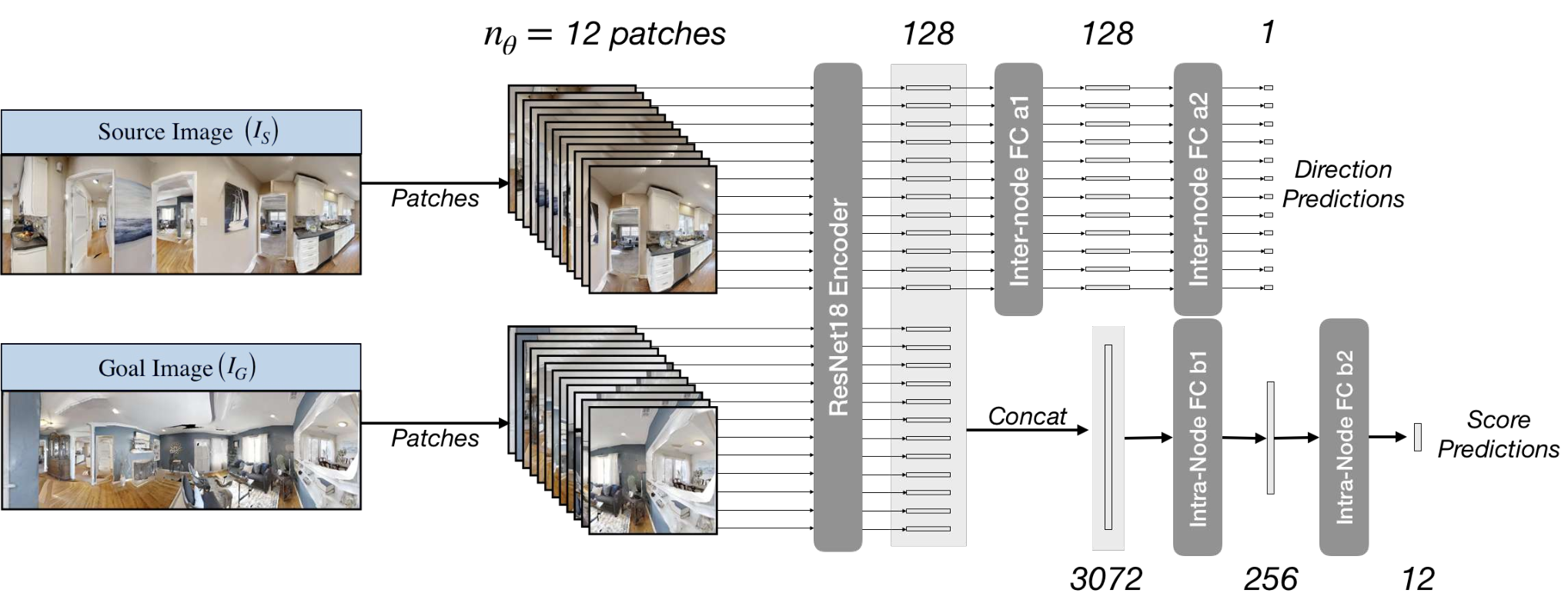
3 Dataset collection and automated labeling
For training the NTS Multi-task Learning model, we need to collect the data and different types of labels. We randomly sample 300 points in each training scene. For each ordered pair of nts/images, source image () and goal image (), we gather the different labels as follow:
Connection label: This label denotes whether the source and goal image belong to the same node or not. We get this label by detecting whether the goal image location is visible from the source image. To compute this, we take a 5-degree patch of depth image centered at the relative direction of the goal image from the source image. If the maximum depth in this patch is greater than the distance to the goal image, then the goal image belongs to the same node as the source image and the label is 1. Intuitively, the above checks whether the maximum depth value in the direction of the goal image is greater than the distance to the goal. If the maximum depth in the direction of goal image is greater than the distance to the goal image or if the distance to the goal image is greater than , then the goal image belongs to a different node and the label is 0.
Intra-node labels: If the source and goal image belong to the same node, i.e. the above label is 1, then the intra-node direction and score labels are directly obtained from relative position of the goal image from the source image. Let the relative position of the goal image be , where is the distance and is the angle to the goal image from the source image. Intra-node direction label is just the degree bin in which falls, i.e. where is the nearest integer function. For the intra-node score label (), we just convert the distance to a score between and using the following function:
where denotes the score, denotes the radius of the node, is the distance. Note that the direction label is discrete and the score label is continuous.
Inter-node labels: If the source and goal image do not belong to the same node, i.e. the connection label is 0, we compute the inter-node labels. For computing the inter-node direction labels, we first project the depth channel in the panoramic source image to compute an obstacle map. We ignore obstacles beyond . In this obstacle map, we take points at angles and distance away. For every, , if the shortest path distance to the corresponding is less than , then the corresponding inter-node direction label is 1 and otherwise 0.
Let the inter-score labels be denoted by . For the inter-node score label , we find the farthest explored and traversable point in direction in the above obstacle map. Let the shortest path distance (geodesic distance) of the goal image from this point be . Then the score label is given by:
where is the maximum distance above which the score is 0.
3 Experimental Setup
Environment. All our experiments are conducted in the Habitat simulator [168] with the Gibson [212] dataset. The Gibson dataset is visually realistic as it consists of reconstructions of real-world scenes. We also implement physically realistic motion sensor and actuation noise models as proposed by [35]. Actuation motion noise leads to stochastic transitions as the amount translated or rotated by the agent is noisy. This model also adds realistic translational noise in rotation actions and rotational noise in translational actions. The sensor noise model adds realistic noise to the base odometry sensor readings. Both the noise models are based on real-world data and agents trained on these noise models are shown to transfer to the real-world [35].
Task setup. We use panoramic nts/images of size for both agent image observation and target goal image. We conduct experiments with both RGB and RGBD settings. The base odometry sensor provides a reading denoting the change in agent’s x-y coordinates and orientation. The action space consists of four actions: move_forward, turn_right, turn_left, stop. The forward action moves the agent approximately 25cm forward and the turn actions turn the agent approximately 10 degrees. Note that the state space and motion of the agent are continuous. The agent succeeds in an episode if it takes the stop action within a radius of the target location. The agent fails if it takes stop action anywhere else or does not take the stop till the episode ends. In addition to the success rate, we also use Success weighted by inverse Path Length (SPL) as an evaluation metric as proposed by [4]. It takes into account the efficiency of the agent in reaching the goal (shorter successful trajectories lead to higher SPL).
Training data. We split the curated set of 86 scenes from [168] into sets of 68/4/14 scenes for train/val/test. For training our supervised learning model, we sample 300 nts/images randomly in each of 68 training scenes. We get labels for pairs of source and target nts/images in each scene giving us a total of approximately = 6.12 million data points. The labeling process is automated and it only requires the ground-truth map already available with the dataset without the need for any additional human annotation. Note that sampling nts/images or the ground-truth map are not required for the test environments.
Test episodes. For creating test episodes, we sample episodes (given by starting and goal locations) in the test scenes to create 3 different sets of difficulty based on the distance of the goal from starting locations: Easy (), Medium () and Hard (). The maximum episode length is 500 steps for each difficulty level.
| Easy | Medium | Hard | Overall | |||||||||
| Model | Succ | SPL | Succ | SPL | Succ | SPL | Succ | SPL | ||||
| RGB | ResNet + GRU + IL | 0.57 | 0.23 | 0.14 | 0.06 | 0.04 | 0.02 | 0.25 | 0.10 | |||
| Target-driven RL | 0.56 | 0.22 | 0.17 | 0.06 | 0.06 | 0.02 | 0.26 | 0.10 | ||||
| Active Neural SLAM (ANS) | 0.63 | 0.45 | 0.31 | 0.18 | 0.12 | 0.07 | 0.35 | 0.23 | ||||
| Neural Topological SLAM (NTS) | 0.80 | 0.60 | 0.47 | 0.31 | 0.37 | 0.22 | 0.55 | 0.38 | ||||
| RGBD | ResNet + GRU + IL | 0.72 | 0.32 | 0.16 | 0.09 | 0.05 | 0.02 | 0.31 | 0.14 | |||
| Target-driven RL | 0.68 | 0.28 | 0.21 | 0.08 | 0.09 | 0.03 | 0.33 | 0.13 | ||||
| Metric Spatial Map + RL | 0.69 | 0.27 | 0.22 | 0.07 | 0.12 | 0.04 | 0.34 | 0.13 | ||||
| Metric Spatial Map + FBE + Local | 0.77 | 0.56 | 0.36 | 0.18 | 0.13 | 0.05 | 0.42 | 0.26 | ||||
| Active Neural SLAM (ANS) | 0.76 | 0.55 | 0.40 | 0.24 | 0.16 | 0.09 | 0.44 | 0.29 | ||||
| Neural Topological SLAM (NTS) | 0.87 | 0.65 | 0.58 | 0.38 | 0.43 | 0.26 | 0.63 | 0.43 | ||||
1 Baselines
We use the following baselines for our experiments:
ResNet + GRU + IL. A simple baseline consisting of ResNet18 image encoder and GRU based policy trained with imitation learning (IL).
Target-driven RL. A siamese style model for encoding the current image and the goal image using shared convolutional networks and trained end-to-end with reinforcement learning, adapted from Zhu et al. [222].
Metric Spatial Map + RL. An end-to-end RL model which uses geometric projections of the depth image to create a local map and passes it to the RL policy, adapted from Chen et al. [41].
Metric Spatial Map + FBE + Local. This is a hand-designed baseline which creates a map using depth nts/images and then uses a classical exploration heuristic called Frontier-based Exploration (FBE) [214] which greedily explores nearest unexplored frontiers in the map. We use the Localization model and Local Policy from NTS to detect when a goal is nearby and navigate to it.
Active Neural SLAM. This is a recent modular model based on Metric Spatial Maps proposed for the task of exploration. We adapt it to the Image Goal task by using the Localization model and Local Policy from NTS to detect when a goal is nearby and navigate to it.
All the baselines are trained for 25 million frames. RL baselines are trained using Proximal Policy Optimization [172] with a dense reward function. The reward function includes a high reward for success (=SPL*10.), a shaping reward equal to the decrease in distance to the goal and a per step reward of -0.001 to encourage shorter trajectories. ResNet + GRU + IL is trained using behavioral cloning on the ground-truth trajectory. This means just like the proposed model, all the baselines also use the ground-truth map for training. In terms of the number of training samples, sampling 300 random nts/images in the environment would require 300 episode resets in the RL training setup. 300 episodes in 68 scenes would lead to a maximum of million () samples. Since we use 25 million frames to train our baselines, they use strictly more data than our model. Furthermore, our model does not require any interaction in the environment and can be trained offline with image data.
| RGBD - No stop | RGBD - No Noise | |||||||||
|---|---|---|---|---|---|---|---|---|---|---|
| Model | Easy | Med. | Hard | Overall | Easy | Med. | Hard | Overall | ||
| ResNet + GRU + IL | 0.76 | 0.28 | 0.10 | 0.38 | 0.71 | 0.18 | 0.06 | 0.32 | ||
| Target-driven RL | 0.89 | 0.45 | 0.21 | 0.52 | 0.69 | 0.22 | 0.07 | 0.33 | ||
| Metric Spatial Map + RL | 0.89 | 0.45 | 0.21 | 0.52 | 0.70 | 0.24 | 0.11 | 0.35 | ||
| Metric Spatial Map + FBE + Local | 0.92 | 0.46 | 0.29 | 0.56 | 0.78 | 0.46 | 0.23 | 0.49 | ||
| Active Neural SLAM (ANS) | 0.93 | 0.50 | 0.32 | 0.58 | 0.79 | 0.53 | 0.30 | 0.54 | ||
| Neural Topological SLAM (NTS) | 0.94 | 0.70 | 0.60 | 0.75 | 0.87 | 0.60 | 0.46 | 0.64 | ||
4 Results
We evaluate the proposed method and all the baselines on 1000 episodes for each difficulty setting. We compare all the methods across all difficulty levels in both RGB and RGBD settings in Table 1. The results show that the proposed method outperforms all the baselines by a considerable margin across all difficulty settings with an overall Succ/SPL of 0.55/0.38 vs 0.35/0.23 in RGB and 0.63/0.43 vs 0.44/0.29 in RGBD. The results also indicate the relative improvement of NTS over the baselines increases as the difficulty increases leading to a large improvement in the hard setting (0.43/0.26 vs 0.16/0.09 in RGBD). In Fig 13, we visualize an example trajectory using the NTS model.
Comparison with end-to-end RL and the effect of stop action. The results indicate that NTS performs better than both end-to-end RL based baselines [222, 41] and methods using metric spatial maps [41, 35]. The performance of the RL-based baselines is much weaker than the proposed model. We believe the reason behind this is the complexity of the exploration search space. Compared to the Pointgoal navigation task where the agent receives updated direction to the goal at each time step, Image Goal navigation is more difficult in terms of exploration as the goal image does not directly provide the direction to explore. Another difficulty is exploring the ‘stop’ action. Prior setups of the Image Goal task where end-to-end RL policies were shown to perform reasonably well assumed that the agent succeeded if it hits the goal state. However, based on the suggestion from [4], we added the ‘stop’ action as it is more realistic. To quantify the effect of stop action, we report the performance of all the models without the stop action in Table 2(left). We see that the performance of RL baselines is much higher. However, the performance of NTS also increases as the agent automatically stops when it reaches the goal state instead of using the prediction of the Relative Pose Estimator to stop. Other differences that make our experimental setup more realistic but also makes exploration harder for RL as compared to prior setups include continuous state space as compared to grid-based state space, fine-grained action as compared to 90 degree turns and grid cell forward steps and stochastic transitions due to realistic motion noise.
Comparison with spatial map-based methods and the effect of motion noise. The performance of metric spatial map-based baselines drops quickly as the distance to the goal increases. This is likely due to the accumulation of pose errors as the trajectory length increases. Errors in pose prediction make the map noisy and eventually lead to incorrect path planning. To quantify this effect, we evaluate all the models without any motion actuation and sensor noise in Table 2(right). The results show that the performance of the metric map-based baselines scales much better with distance in the absence of motion noise, however, the performance of NTS does not increase much. This indicates that NTS is able to tackle motion noise relatively well. This is because NTS only uses pose estimates between consecutive nodes, which do not accumulate much noise as they are a few actions away from each other. The performance of NTS is still better than the baselines even without motion noise as it consists of Semantic Score Predictor () capable of learning structural priors which the metric spatial map-based baselines lack. We quantify the effect of the Semantic Score Predictor in the following subsection.
1 Ablations and Sequential Goals
In this subsection, we evaluate the proposed model on sequential goals in a single episode and study the importance of the topological map or the graph and the Semantic Score Predictor (). For creating a test episode with sequential goals, we randomly sample a goal between to away from the last goal. The agent gets a time budget of 500 timesteps for each goal. We consider two ablations:
NTS w/o Graph. We pick the direction with the highest score in the current image greedily, not updating or using the graph over time. Intuitively, the performance of this ablation should deteriorate as the number of sequential goals increases as it has no memory of past observations.
Neural Topological SLAM w/o Score Function. In this ablation, we do not use the Semantic Score Predictor () and pick a ghost node randomly as the long-term goal when the Goal Image is not localized in the current graph. Intuitively, the performance of this ablation should improve with the increase in the number of sequential goals, as random exploration would build the graph over time and increase the likelihood of the Goal Image being localized.
We report the success rate and SPL of NTS and the two ablations as a function of the number of sequential goals in Figure 12. Success, in this case, is defined as the ratio of goals reached by the agent across a test set of 1000 episodes. The performance of NTS is considerably higher than both the ablations, indicating the importance of both the components. The drop in performance when the semantic score function is removed indicates that the model learns some semantic priors (Figure 14 shows an example). The performance of all the models decreases with an increase in the number of sequential goals because if the agent fails to reach an intermediate goal, there is a high chance that the subsequent goals are farther away. The performance gap between NTS and NTS w/o Score Function decreases and the performance gap between NTS and NTS w/o Graph increases with increase in the number of sequential goals as expected. This indicates that the topological map becomes more important over time as the agent explores a new environment, and while the Semantic Score Predictor is the most important at the beginning to explore efficiently.
5 Discussion
We designed topological representations for space that leverage semantics and afford coarse geometric reasoning. We showed how we can build such representation autonomously and use them for the task of image-goal navigation. Topological representations provided robustness to actuation noise, while semantic features stored at nodes allowed the use of statistical regularities for efficient exploration in novel environments. We showed how advances made in this paper make it possible to study this task in settings where no prior experience from the environment is available, resulting in a relative improvement of over .
Neural Topological SLAM encodes the semantics in the map implicitly using localization and semantic score functions and tackles the Image Goal Navigation task. In the next chapter, we will present methods which encode semantics in the map explicitly and study them in the context of the Object Goal Navigation task.


Chapter 6 Goal-Oriented Semantic Exploration
00footnotetext: Webpage: https://devendrachaplot.github.io/projects/semantic-explorationConsider an autonomous agent being asked to navigate to a ‘dining table’ in an unseen environment as shown in Figure 1. In terms of semantic understanding, this task not only involves object detection, i.e. what does a ‘dining table’ look like, but also scene understanding of where ‘dining tables’ are more likely to be found. The latter requires a long-term episodic memory as well as learning semantic priors on the relative arrangement of objects in a scene. Long-term episodic memory allows the agent to keep track of explored and unexplored areas. Learning semantic priors allows the agent to also use the episodic memory to decide which region to explore next in order to find the target object in the least amount of time.
How do we design a computational model for building an episodic memory and using it effectively based on semantic priors for efficient navigation in unseen environments? One popular approach is to use end-to-end reinforcement or imitation learning with recurrent neural networks to build episodic memory and learn semantic priors implicitly [137, 81, 222, 143]. However, end-to-end learning-based methods suffer from large sample complexity and poor generalization as they memorize object locations and appearance in training environments.
In Chapter 4, we introduced a modular learning-based system called ‘Active Neural SLAM’ which builds explicit obstacle maps to maintain episodic memory. Explicit maps also allow analytical path planning and thus lead to significantly better exploration and sample complexity. However, Active Neural SLAM, designed for maximizing exploration coverage, does not encode semantics in the episodic memory and thus does not learn semantic priors. In this chapter, we extend the Active Neural SLAM system to build explicit semantic maps and learn semantic priors using a semantically-aware long-term policy.

The proposed method, called ‘Goal-Oriented Semantic Exploration’ (SemExp), makes two improvements over Active Neural SLAM [35] to tackle semantic navigation tasks. First, it builds top-down metric maps similar to [35] but adds extra channels to encode semantic categories explicitly. Instead of predicting the top-down maps directly from the first-person image as in [35], we use first-person predictions followed by differentiable geometric projections. This allows us to leverage existing pretrained object detection and semantic segmentation models to build semantic maps instead of learning from scratch. Second, instead of using a coverage maximizing goal-agnostic exploration policy based only on obstacle maps, we train a goal-oriented semantic exploration policy which learns semantic priors for efficient navigation. These improvements allow us to tackle a challenging object goal navigation task. Our experiments in visually realistic simulation environments show that SemExp outperforms prior methods by a significant margin. The proposed model also won the CVPR 2020 Habitat ObjectNav Challenge [15]11 1 https://aihabitat.org/challenge/2020/. We also demonstrate that SemExp achieves similar performance in the real-world when transferred to a mobile robot platform.
We briefly discuss related work on semantic mapping and navigation below.
Semantic Mapping. There’s a large body of work on building obstacle maps both in 2D and 3D using structure from motion and Simultaneous Localization and Mapping (SLAM) [88, 96, 180]. We defer the interested readers to the survey by Fuentes-Pacheco et al. 2015 [71] on SLAM. Some of the more relevant works incorporate semantics in the map using probabilistic graphical models [22] or using recent learning-based computer vision models [221, 130]. In contrast to these works, we use differentiable projection operations to learn semantic mapping with supervision in the map space. This limits large errors in the map due to small errors in first-person semantic predictions.
Navigation. Classical navigation approaches use explicit geometric maps to compute paths to goal locations via path planning [104, 121, 26, 174]. The goals are selected base on heuristics such as the Frontier-based Exploration algorithm [214]. In contrast, we use a learning-based policy to use semantic priors for selecting exploration goals based on the object goal category.
Recent learning-based approaches use end-to-end reinforcement or imitation learning for training navigation policies. These include methods which use recurrent neural networks [137, 120, 31, 167, 89, 34, 168, 204], structured spatial representations [81, 153, 33, 87, 78] and topological representations [165, 166]. Recent works tackling object goal navigation include [206, 216, 205, 143]. Wu et al. 2018 [206] try to explore structural similarities between the environment by building a probabilistic graphical model over the semantic information like room types. Similarly, Yang et al. 2018 [216] propose to incorporate semantic priors into a deep reinforcement learning framework by using Graph Convolutional Networks. Wortsman et al. 2019 [205] propose a meta-reinforcement learning approach where an agent learns a self-supervised interaction loss that encourages effective navigation to even keep learning in a test environment. Mousavian et al. 2019 [143] use semantic segmentation and detection masks obtained by running state-of-the-art computer vision algorithms on the input observation and used a deep network to learn the navigation policy based on it. In all the above methods, the learnt representations are implicit and the models need to learn obstacle avoidance, episodic memory, planning as well as semantic priors implicitly from the goal-driven reward. Explicit map representation has been shown to improve performance as well as sample efficiency over end-to-end learning-based methods for different navigation tasks [35, 37], however they learn semantics implicitly. In this work, we use explicit structured semantic map representation, which allows us to learn semantically-aware exploration policies and tackle the object-goal navigation task. Concurrent work studies the use of similar semantic maps in learning exploration policies for improving object detection systems [36].
1 Problem Definition
In the Object Goal task [167, 4], the objective is to navigate to an instance of the given object category such as ‘chair’ or ‘bed’. The agent is initialized at a random location in the environment and receives the goal object category () as input. At each time step , the agent receives visual observations () and sensor pose readings and takes navigational actions . The visual observations consist of first-person RGB and depth images. The action space consists of four actions: move_forward, turn_left, turn_right, stop. The agent needs to take the ‘stop’ action when it believes it has reached close to the goal object. If the distance to the goal object is less than some threshold, , when the agent takes the stop action, the episode is considered successful. The episode terminates at after a fixed maximum number of timesteps .
2 Methods
We propose a modular model called ‘Goal-Oriented Semantic Exploration’ (SemExp) to tackle the Object Goal navigation task (see Figure 2 for an overview). It consists of two learnable modules, ‘Semantic Mapping’ and ‘Goal-Oriented Semantic Policy’. The Semantic Mapping module builds a semantic map over time and the Goal-Oriented Semantic Policy selects a long-term goal based on the semantic map to reach the given object goal efficiently. A deterministic local policy based on analytical planners is used to take low-level navigation actions to reach the long-term goal. We first describe the semantic map representation used by our model and then describe the modules.
Semantic Map Representation. The SemExp model internally maintains a semantic metric map, and pose of the agent . The spatial map, , is a matrix where denotes the map size and each element in this spatial map corresponds to a cell of size () in the physical world. is the number of channels in the semantic map, where is the total number of semantic categories. The first two channels represent obstacles and explored area and the rest of the channels each represent an object category. Each element in a channel represents whether the corresponding location is an obstacle, explored, or contains an object of the corresponding category. The map is initialized with all zeros at the beginning of an episode, . The pose denotes the and coordinates of the agent and the orientation of the agent at time . The agent always starts at the center of the map facing east at the beginning of the episode, .
Semantic Mapping. In order to a build semantic map, we need to predict semantic categories and segmentation of the objects seen in visual observations. It is desirable to use existing object detection and semantic segmentation models instead of learning from scratch. The Active Neural SLAM model predicts the top-down map directly from RGB observations and thus, does not have any mechanism for incorporating pretrained object detection or semantic segmentation systems. Instead, we predict semantic segmentation in the first-person view and use differentiable projection to transform first-person predictions to top-down maps. This allows us to use existing pretrained models for first-person semantic segmentation. However small errors in first-person semantic segmentation can lead to large errors in the map after projection. We overcome this limitation by imposing a loss in the map space in addition to the first-person space.
Figure 3 shows an overview of the Semantic Mapping module. The
depth observation is used to compute a point cloud. Each point in the point cloud is associated with the predicted semantic categories. The semantic categories are predicted using a pretrained Mask RCNN [84] on the RGB observation. Each point in the point cloud is then projected in 3D space using differentiable geometric computations to get the voxel representation. The voxel representation is then converted to the semantic map. Summing over the height dimension of the voxel representation for all obstacles, all cells, and each category gives different channels of the projected semantic map. The projected semantic map is then passed through a denoising neural network to get the final semantic map prediction. The map is aggregated over time using spatial transformations and channel-wise pooling as described in [35]. The Semantic Mapping module is trained using supervised learning with cross-entropy loss on the semantic segmentation as well as semantic map prediction. The geometric projection is implemented using differentiable operations such that the loss on the semantic map prediction can be backpropagated through the entire module if desired.

Goal-Oriented Semantic Policy. The Goal-Oriented Semantic Policy decides a long-term goal based on the current semantic map to reach the given object goal (). If the channel corresponding to category has a non-zero element, meaning that the object goal is observed, it simply selects all non-zero elements as the long-term goal. If the object goal is not observed, the Goal-Oriented Semantic Policy needs to select a long-term goal where a goal category object is most likely to be found. This requires learning semantic priors on the relative arrangement of objects and areas. We use a neural network to learn these semantic priors. It takes the semantic map, the agent’s current and past locations, and the object goal as input and predicts a long-term goal in the top-down map space.
The Goal-Oriented Semantic Policy is trained using reinforcement learning with distance reduced to the nearest goal object as the reward. We sample the long-term goal at a coarse time-scale, once every steps, similar to the goal-agnostic Global Policy in [35]. This reduces the time-horizon for exploration in RL exponentially and consequently, reduces the sample complexity.
Deterministic Local Policy. The local policy uses Fast Marching Method [174] to plan a path to the long-term goal from the current location based on the obstacle channel of the semantic map. It simply takes deterministic actions along the path to reach the long-term goal. We use a deterministic local policy as compared to a trained local policy in [35] as they led to a similar performance in our experiments. Note that although the above Semantic Policy acts at a coarse time scale, the Local Policy acts at a fine time scale. At each time step, we update the map and replan the path to the long-term goal.
3 Experimental Setup
We use the Gibson [212] and Matterport3D (MP3D) [29] datasets in the Habitat simulator [168] for our experiments. Both Gibson and MP3D consist of scenes which are 3D reconstructions of real-world environments. For the Gibson dataset,wWe use the train and val splits of Gibson tiny set for training and testing respectively as the test set is held-out for the online evaluation server. We do not use the validation set for hyper-parameter tuning. The semantic annotations for the Gibson tiny set are available from Armeni et al. 2019 [6]. For the MP3D dataset, we use the standard train and test splits. Our training and test set consists of a total of 86 scenes (25 Gibson tiny and 61 MP3D) and 16 scenes (5 Gibson tiny and 11 MP3D), respectively.
The observation space consists of RGBD images of size , base odometry sensor readings of size denoting the change in agent’s x-y coordinates and orientation, and goal object category represented as an integer. The actions space consists of four actions: move_forward, turn_left, turn_right, stop. The success threshold is set to . The maximum episode length is 500 steps. We note that the depth and pose are perfect in simulation, but these challenges are orthogonal to the focus of this chapter and prior works have shown that both can be estimated effectively from RGB images and noisy sensor pose readings [77, 35]. These design choices are identical to the CVPR 2020 Object Goal Navigation Challenge.
For the object goal, we use object categories which are common between Gibson, MP3D, and MS-COCO [128] datasets. This leads to set of 6 object goal categories: ‘chair’, ‘couch’, ‘potted plant’, ‘bed’, ‘toilet’ and ‘tv’. We use a Mask-RCNN [84] using Feature Pyramid Networks [129] with ResNet50 [85] backbone pretrained on MS-COCO for object detection and instance segmentation. Although we use 6 categories for object goals, we build a semantic map with 15 categories (shown on the right in Figure 4) to encode more information for learning semantic priors.

Architecture and Hyperparameter details. We use PyTorch [154] for implementing and training our model. The denoising network in the Semantic Mapping module is a 5-layer fully convolutional network. We freeze the Mask RCNN weights in the Semantic Mapping module (except for results on Habitat Challenge in Section 2) as Matterport does not contain labels for all 15 categories in our semantic map. We train the denoising network with the map-based loss on all 15 categories for Gibson frames and only 6 categories on MP3D frames. The Goal-driven Semantic Policy is a 5 layer convolutional network followed by 3 fully connected layers. In addition to the semantic map, we also pass the agent orientation and goal object category index as separate inputs to this Policy. They are processed by separate Embedding layers and added as an input to the fully-connected layers.
We train both the modules with 86 parallel threads, with each thread using one scene in the training set. We maintain a FIFO memory of size 500000 for training the Semantic Mapping module. After one step in each thread, we perform 10 updates to the Semantic Mapping module with a batch size of 64. We use Adam optimizer with a learning rate of . We use binary cross-entropy loss for semantic map prediction. The Goal-driven Policy samples a new goal every timesteps. For training this policy, we use Proximal Policy Optimization (PPO) [172] with a time horizon of 20 steps, 36 mini-batches, and 4 epochs in each PPO update. Our PPO implementation is based on [112]. The reward for the policy is the decrease in distance to the nearest goal object. We use Adam optimizer with a learning rate of , a discount factor of , an entropy coefficient of , value loss coefficient of for training the Goal-driven Policy.
Metrics. We use 3 metrics for comparing all the methods: Success. Ratio of episodes where the method was successful. SPL. Success weighted by Path Length as proposed by [4]. This metric measures the efficiency of reaching the goal in addition to the success rate. DTS: Distance to Success. This is the distance of the agent from the success threshold boundary when the episode ends. This is computed as follows:
where is the L2 distance of the agent from the goal location at the end of the episode, is the success threshold.
1 Baselines.
We use two end-to-end Reinforcement Learning (RL) methods as baselines:
RGBD + RL: A vanilla recurrent RL Policy initialized with ResNet18 [85] backbone followed by a GRU adapted from Savva et al. 2019 [168]. Agent pose and goal object category are passed through an embedding layer and append to the recurrent layer input.
RGBD + Semantics + RL [143]: This baseline is adapted from Mousavian et al. 2019 [143] who pass semantic segmentation and object detection predictions along with RGBD input to a recurrent RL policy. We use a pretrained Mask RCNN identical to the one used in the proposed model for semantic segmentation and object detection in this baseline. RGBD observations are encoded with a ResNet18 backbone visual encoder, and agent pose and goal object are encoded usinng embedding layers as described above.
Both the RL based baselines are trained with Proximal Policy Optimization [172] using a dense reward of distance reduced to the nearest goal object. We design two more baselines based on goal-agnostic exploration methods combined with heuristic-based local goal-driven policy.
Classical Mapping + FBE [214]: This baseline use classical robotics pipeline for mapping followed by classical frontier-based exploration (FBE) [214] algorithm. We use a heuristic-based local policy using a pretrained Mask-RCNN. Whenever the Mask RCNN detects the goal object category, the local policy tries to go towards the object using an analytical planner.
Active Neural SLAM [35]: In this baseline, we use an exploration policy trained to maximize coverage from [35], followed by the heuristic-based local policy as described above.
| Gibson | MP3D | |||||||
|---|---|---|---|---|---|---|---|---|
| Method | SPL | Success | DTS (m) | SPL | Success | DTS (m) | ||
| Random | 0.004 | 0.004 | 3.893 | 0.005 | 0.005 | 8.048 | ||
| RGBD + RL | 0.027 | 0.082 | 3.310 | 0.017 | 0.037 | 7.654 | ||
| RGBD + Semantics + RL | 0.049 | 0.159 | 3.203 | 0.015 | 0.031 | 7.612 | ||
| Classical Map + FBE | 0.124 | 0.403 | 2.432 | 0.117 | 0.311 | 7.102 | ||
| Active Neural SLAM | 0.145 | 0.446 | 2.275 | 0.119 | 0.321 | 7.056 | ||
| SemExp | 0.199 | 0.544 | 1.723 | 0.144 | 0.360 | 6.733 | ||
4 Results
We train all the baselines and the proposed model for 10 million frames and evaluate them on the Gibson and MP3D scenes in our test set separately. We run 200 evaluations episode per scene, leading to a total of 1000 episodes in Gibson (5 scenes) and 2000 episodes in MP3D (10 scenes, 1 scene did not contain any object of the 6 possible categories). Figure 4 visualizes an exmaple trajectory using the proposed SemExp showing the agent observations and predicted semantic map22 2 See demo videos at https://devendrachaplot.github.io/projects/semantic-exploration. The quantitative results are shown in Table 1. SemExp outperforms all the baselines by a considerable margin consistently across both the datasets (achieving a success rate 54.4%/36.0% on Gibson/MP3D vs 44.6%/32.1% for the Active Neural SLAM baseline) . The absolute numbers are higher on the Gibson set, as the scenes are comparatively smaller. The Distance to Success (DTS) threshold for Random in Table 1 indicates the difficulty of the dataset. Interestingly, the baseline combining classical exploration with pretrained object detectors outperforms the end-to-end RL baselines. We observed that the training performance of the RL-based baselines was much higher indicating that they memorize the object locations and appearance in the training scenes and generalize poorly. The increase in performance of SemExp over the Active Neural SLAM baseline shows the importance of incorporating semantics and the goal object in exploration.
| Method | SPL | Success | DTS (m) | |
|---|---|---|---|---|
| SemExp w.o. Semantic Map | 0.165 | 0.488 | 2.084 | |
| SemExp w.o. Goal Policy | 0.148 | 0.450 | 2.315 | |
| SemExp | 0.199 | 0.544 | 1.723 | |
| SemExp w. GT SemSeg | 0.457 | 0.731 | 1.089 |

1 Ablations and Error Analysis
To understand the importance of both the modules in SemExp, we consider two ablations:
SemExp w.o. Semantic Map. We replace the Semantic Map with the Obstacle-only Map. As opposed to the Active Neural SLAM baseline, the Goal-oriented Policy is still trained with distance reduced to the nearest object as the reward.
SemExp w.o. Goal Policy. We replace the Goal-driven policy with a goal-agnostic policy trained to maximize exploration coverage as in [35], but still trained with the semantic map as input.
The results in the top part of Table 2 show the performance of these ablations. The performance of SemExp without the Goal-oriented policy is comparable to the Active Neural SLAM baseline, indicating that the Goal-oriented policy learns semantic priors for better exploration leading to more efficient navigation. Figure 5 shows an qualitative example indicating the importance of the Goal-oriented Policy. The performance of SemExp without the Semantic Map also drops, but it is higher than the ablation without Goal Policy. This indicates that it is possible to learn some semantic priors with just the obstacle map without semantic channels.
The performance of the proposed model is still far from perfect. We would like to understand the error modes for future improvements. We observed two main sources of errors, semantic segmentation inaccuracies and inability to find the goal object. In order to quantify the effect of both the error modes, we evaluate the proposed model with ground truth semantic segmentation (see SemExp w. GT SemSeg in Table 2) using the ‘Semantic’ sensor in Habitat simulator. This leads to a success rate of 73.1% vs 54.4%, which means around 19% performance can be improved with better semantic segmentation. The rest of the 27% episodes are mostly cases where the goal object is not found, which can be improved with better semantic exploration.
2 Result on Habitat Challenge
SemExp also won the CVPR 2020 Habitat ObjectNav Challenge. The challenge task setup is identical to ours except the goal object categories. The challenge uses 21 object categories for the goal object. As these object categories are not overlapping with the COCO categories, we use DeepLabv3 [40] model for semantic segmentation. We predict the semantic segmentation and the semantic map with all 40 categories in the MP3D dataset including the 21 goal categories. We fine-tune the DeepLabv3 segmentation model by retraining the final layer to predict semantic segmentation for all 40 categories. This segmentation model is also trained with the map-based loss in addition to the first-person segmentation loss. The performance of the top 5 entries to the challenge are shown in Table 3. The proposed approach outperforms all the other entries with a success rate of 25.3% as compared to 18.8% for the second place entry.
| Team Name | SPL | Success | Dist To Goal (m) | |
|---|---|---|---|---|
| SemExp | 0.102 | 0.253 | 6.328 | |
| SRCB-robot-sudoer | 0.099 | 0.188 | 6.908 | |
| Active Exploration (Pre-explore) | 0.046 | 0.126 | 7.336 | |
| Black Sheep | 0.028 | 0.101 | 7.033 | |
| Blue Ox | 0.021 | 0.069 | 7.233 |

3 Real World Transfer
We used the Locobot hardware platform and PyRobot API [146] to deploy the trained policy in the real world. In Figure 6 we show an episode of the robot when it was provided ‘potted plant’ as the object goal. The long-term goals sampled by the Goal-driven policy (shown by blue circles on the map) are often towards spaces where there are high chances of finding a potted plant. This indicates that it is learning to exploit the structure in the semantic map to some extent. Out of 20 trials in the real-world, our method succeeded in 13 episodes leading to a success rate of 65%. End-to-end learning-based policies failed consistently in the real-world due to the visual domain gap between simulation environments and the real-world. Our model performs well in the real-world as (1) it is able to leverage Mask RCNN which is trained on real-world data and (2) the other learned modules (map denoising and the goal policy) work on top-down maps which are domain-agnostic. Our trials in the real-world also indicate that perfect pose and depth are not critical to the success of our model as it can be successfully transferred to the real-world where pose and depth are noisy.
5 Discussion
In this chapter, we presented a semantically-aware exploration model to tackle the object goal navigation task in large realistic environments. The proposed model makes two major improvements over prior methods, incorporating semantics in explicit episodic memory and learning goal-oriented semantic exploration policies. Our method achieves state-of-the-art performance on the object goal navigation task and won the CVPR2020 Habitat ObjectNav challenge. Ablation studies show that the proposed model learns semantic priors which lead to more efficient goal-driven navigation. Domain-agnostic module design led to successful transfer of our model to the real-world. We also analyze the error modes for our model and quantify the scope for improvement along two important dimensions (semantic mapping and goal-oriented exploration) in the future work. The proposed model can also be extended to tackle a sequence of object goals by utilizing the episodic map for more efficient navigation for subsequent goals.
The semantic mapping learnt by the SemExp model can also be used for active visual learning, where an embodied agent actively explores the environment to collect observations to learn and improve perception models. In the next chapter, we explore a self-supervised approach for training an exploration policy for improving an object detection model.
Chapter 7 Semantic Curiosity
00footnotetext: Webpage: https://devendrachaplot.github.io/projects/SemanticCuriosityImagine an agent whose goal is to learn how to detect and categorize objects. How should the agent learn this task? In the case of humans (especially babies), learning is quite interactive in nature. We have the knowledge of what we know and what we don’t, and we use that knowledge to guide our future experiences/supervision. Compare this to how current algorithms learn – we create datasets of random images from the internet and label them, followed by model learning. The model has no control over what data and what supervision it gets – it is resigned to the static biased dataset of internet images. Why does current learning look quite different from how humans learn? During the early 2000s, as data-driven approaches started to gain acceptance, the computer vision community struggled with comparisons and knowing which approaches work and which don’t. As a consequence, the community introduced several benchmarks from BSDS [131] to VOC [60]. However, a negative side effect of these benchmarks was the use of static training and test datasets. While the pioneering works in computer vision focused on active vision and interactive learning, most of the work in the last two decades focuses on static internet vision. But as things start to work on the model side, we believe it is critical to look at the big picture again and return our focus to an embodied and interactive learning setup.
In an embodied interactive learning setup, an agent has to perform actions such that observations generated from these actions can be useful for learning to perform the semantic task. Several core research questions need to be answered: (a) what is the policy of exploration that generates these observations? (b) what should be labeled in these observations - one object, one frame, or the whole trajectory? (c) and finally, how do we get these labels? In this chapter, we focus on the first task – what should the exploration policy be to generate observations which can be useful in training an object detector? Instead of using labels, we focus on learning these trajectories in an unsupervised/self-supervised manner. Once the policy has been learned, we use the policy in novel (previously unseen) scenes to perform actions. As observations are generated, we assume that an oracle will densely label all the objects of interest in the trajectories.
So what are the characteristics of a good exploration policy for visual learning, and how do we learn it? A good semantic exploration policy is one which generates observations of objects and not free-space or the wall/ceiling. But not only should the observations be objects, but a good exploration policy should also observe many unique objects. Finally, a good exploration policy will move to parts of the observation space where the current object detection model fails or does not work. Given these characteristics, how should we define a reward function that could be used to learn this exploration policy? Note, as one of the primary requirements, we assume the policy is learned in a self-supervised manner – that is, we do not have ground-truth objects labeled which can help us figure out where the detections work or fail.
Inspired by recent work in intrinsic motivation and curiosity for training policies without external rewards [155, 157], we propose a new intrinsic reward called semantic curiosity that can be used for the exploration and training of semantic object detectors. In the standard curiosity reward, a policy is rewarded if the predicted future observation does not match the true future observation. The loss is generally formulated in the pixel-based feature space. A corresponding reward function for semantic exploration would be to compare semantic predictions with the current model and then confirm with ground-truth labels – however, this requires external labels (and hence is not self-supervised anymore). Instead, we formulate semantic curiosity based on the meta-supervisory signal of consistency in semantic prediction – that is, if our model truly understands the object, it should predict the same label for the object even as we move around and change viewpoints. Therefore, we exploit consistency in label prediction to reward our policies. Our semantic curiosity rewards trajectories which lead to inconsistent labeling behavior of the same object by the semantic classifier. Our experiments indicate that training an exploration policy via semantic curiosity generalizes to novel scenes and helps train an object detector which outperforms baselines trained with other possible alternatives such as random exploration, pixel curiosity, and free space/map curiosity. We also perform a large set of experiments to understand the behavior of a policy trained with semantic curiosity.
We study the problem of how to sample training data in embodied contexts. This is related to active learning (picking what sample to label), active perception (how to move around to gain more information), intrinsic motivation (picking what parts of the environment to explore). Learning in embodied contexts can also leverage spatio-temporal consistency. We survey these research areas below.
Active Perception. Active perception [12] refers to the problem of actively moving the sensors around at test time to improve performance on the task by gaining more information about the environment. This has been instantiated in the context of object detection [3], amodal object detection [215], scene completion [99], and localization [33, 69]. We consider the problem in a different setting and study how to efficiently move around to best learn a model. Furthermore, our approach to learn this movement policy is self-supervised and does not rely on end-task rewards, which were used in [99, 33, 215].
Active Learning. Our problem is more related to that of active learning [175], where an agent actively acquires labels for unlabeled data to improve its model at the fastest rate [173, 73, 217]. This has been used in a number of applications such as medical image analysis [119], training object detectors [198, 216], video segmentation [66], and visual question answering [140]. Most works tackle the setting in which the unlabeled data has already been collected. In contrast, we study learning a policy for efficiently acquiring effective unlabeled data, which is complementary to such active learning efforts.
Intrinsic Rewards. Our work is also related to work on exploration in reinforcement learning [170, 184, 8, 98]. The goal of these works is to effectively explore a Markov Decision Process to find high reward paths. A number of works formulate this as a problem of maximizing an intrinsic reward function which is designed to incentivize the agent to seek previously unseen [61] or poorly understood [155] parts of the environment. This is similar to our work, as we also seek poorly understood parts of the environment. However, we measure this understanding via multi-view consistency in semantics. This is in a departure from existing works that measure it in 2D image space [155], or consistency among multiple models [157]. Furthermore, our focus is not effective exhaustive exploration, but exploration for the purpose of improving semantic models.
Spatio-Temporal smoothing at test time. A number of papers use spatio-temporal consistency at test time for better and more consistent predictions [28, 72]. Much like the distinction from active perception, our focus is using it to generate better data at train time.
Spatio-temporal consistency as training signal. Labels have been propagated in videos to simplify annotations [199], improve prediction performance given limited data [10, 18], as well as collect images [42]. This line of work leverages spatio-temporal consistency to propagate labels for more efficient labeling. Researchers have also used multi-view consistency to learn about 3D shape from weak supervision [196]. We instead leverage spatio-temporal consistency as a cue to identify what the model does not know. [177] is more directly related, but we tackle the problem in an embodied context and study how to navigate to gather the data, rather than analyzing passive datasets for what labels to acquire.
Visual Navigation and Exploration. Prior work on visual navigation can broadly be categorized into two classes based on whether the location of the goal is known or unknown. Navigation scenarios, where the location of the goal is known, include the most common pointgoal task where the coordinate to the goal is given [81, 167]. Another example of a task in this category is vision and language navigation [5] where the path to the goal is described in natural language. Tasks in this category do not require exhaustive exploration of the environment as the location of the goal is known explicitly (coordinates) or implicitly (path).
Navigation scenarios, where the location of the goal is not known, include a wide variety of tasks. These include navigating to a fixed set of objects [120, 58, 209, 31, 137, 81], navigating to an object specified by language [89, 34] or by an image [222, 37], and navigating to a set of objects in order to answer a question [52, 78]. Tasks in this second category essentially involve efficiently and exhaustively exploring the environment to search the desired object. However, most of the above approaches overlook the exploration problem by spawning the target a few steps away from the goal and instead focus on other challenges. For example, models for playing FPS games [120, 58, 209, 31] show that end-to-end RL policies are effective at reactive navigation and short-term planning such as avoiding obstacles and picking positive reward objects as they randomly appear in the environment. Other works show that learned policies are effective at tackling challenges such as perception (in recognizing the visual goal) [222, 37], grounding (in understanding the goal described by language) [89, 34] or reasoning (about visual properties of the target object) [52, 78]. While end-to-end reinforcement learning is shown to be effective in addressing these challenges, they are ineffective at exhaustive exploration and long-term planning in a large environment as the exploration search space increases exponentially as the distance to the goal increases.
Some very recent works explicitly tackle the problem of exploration by training end-to-end RL policies maximizing the explored area [35, 41, 63]. The difference between these approaches and our method is twofold: first, we train semantically-aware exploration policies as compared spatial coverage maximization in some prior works [35, 41], and second, we train our policy in an unsupervised fashion, without requiring any ground truth labels from the simulator as compared to prior works trained using rewards based on ground-truth labels [63].
1 Overview
Our goal is to learn an exploration policy such that if we use this policy to generate trajectories in a novel scene (and hence observations) and train the object detector from the trajectory data, it would provide a robust, high-performance detector. In literature, most approaches use on-policy exploration; that is, they use the external reward to train the policy itself. However, training an action policy to sample training data for object recognition requires labeling objects. Specifically, these approaches would use the current detector to predict objects and compare them to the ground-truth; they reward the policy if the predictions do not match the ground-truth (the policy is being rewarded to explore regions where the current object detection model fails). However, training such a policy via semantic supervision and external rewards would have a huge bottleneck of supervision. Given that our RL policies require millions of samples (in our case, we train using 10M samples), using ground-truth supervision is clearly not the way. What we need is an intrinsic motivation reward that can help train a policy which can help sample training data for object detectors.
We propose a semantic curiosity formulation. Our work is inspired by a plethora of efforts in active learning [175] and recent work on intrinsic reward using disagreement [157]. The core idea is simple – a good object detector has not only high mAP performance but is also consistent in predictions. That is, the detector should predict the same label for different views of the same object. We use this meta-signal of consistency to train our action policy by rewarding trajectories that expose inconsistencies in an object detector. We measure inconsistencies by measuring temporal entropy of prediction – that is, if an object is labeled with different classes as the viewpoint changes, it will have high temporal entropy. The trajectories with high temporal entropy are then labeled via an oracle and used as the data to retrain the object detector (See Figure 2).
2 Methodology
Consider an agent which can perform actions in environments . The agent has an exploration policy that predicts the action that the agent must take for current observation . represents the parameters of the policy that have to be learned. The agent also has an object detection model which takes as input an image (the current observation) and generates a set of bounding boxes along with their categories and confidence scores.
The goal is to learn an exploration policy , which is used to sample trajectories in a set of novel environments (and get them semantically labeled). When used to train an object detector, this labeled data would yield a high-performance object detector. In our setup, we divide the environments into three non-overlapping sets – the first set is the set of environments where the agent will learn the exploration policy , the second set is the object detection training environments where we use to sample trajectories and label them, and the third set is the test environment where we sample random images and test the performance of the object detector on those images.
1 Semantic Curiosity Policy
We define semantic curiosity as the temporal inconsistency in object detection and segmentation predictions from the current model. We use a Mask RCNN to obtain the object predictions. In order to associate the predictions across frames in a trajectory, we use a semantic mapping module as described below.
Semantic Mapping. The Semantic Mapping module takes in a sequence of RGB () and Depth () images and produces a top-down semantic map () represented by a 3-dimensional tensor , where is the length of the square top-down map, and is the number of semantic categories. Each element in this semantic map is if the Mask RCNN predicted the object category at coordinates on the map in any frame during the whole trajectory and otherwise. Figure 3 shows how the semantic map is generated for a single frame. The input RGB frame () is passed through a current Mask RCNN to obtain object segmentation predictions, while the Depth frame is used to calculate the point cloud. Each point in the point cloud is associated with its semantic labels based on Mask RCNN predictions. Note that these are not ground-truth labels, as each pixel is assigned the category of the highest-confidence Mask RCNN segmentation prediction on the corresponding pixel. The point cloud with the associated semantic labels is projected to a 3-dimensional voxel map using geometric computations. The voxel representation is converted to a top-down map by max-pooling the values across the height. The resulting 2D map is converted to a 3-dimensional Semantic Map, such that each channel represents an object category.
The above gives a first-person egocentric projection of the semantic map at each time-step. The egocentric projections at each time step are used to compute a geocentric map over time using a spatial transformation technique similar to Chaplot et al. [35]. The egocentric projections are converted to the geocentric projections by doing a spatial transformation based on the agent pose. The semantic map at each time step is computed by pooling the semantic map at the previous timestep with the current geocentric prediction. Please refer to [35] for more details on these transformations.
Semantic Curiosity Reward. The semantic map allows us to associate the object predictions across different frames as the agent is moving. We define the semantic curiosity reward based on the temporal inconsistency of the object predictions. If an object is predicted to have different labels across different frames, multiple channels in the semantic map at the coordinates corresponding to the object will have s. Such inconsistencies are beneficial for visual learning in downstream tasks, and hence, favorable for the semantic curiosity policy. Thus, we define the cumulative semantic curiosity reward to be proportional to the sum of all the elements in the semantic map. Consequently, the semantic curiosity reward per step is just the increase in the sum of all elements in the semantic map as compared to the previous time step:
where is the semantic curiosity reward coefficient. Summation over the channels encourages exploring frames with temporally inconsistent predictions. Summation across the coordinates encourages exploring as many objects with temporally inconsistent predictions as possible.
The proposed Semantic Curiosity Policy is trained using reinforcement learning to maximize the cumulative semantic curiosity reward. Note that although the depth image and agent pose are used to compute the semantic reward, we train the policy only on RGB images.
3 Experimental Setup
We use the Habitat simulator [168] with three different datasets for our experiments: Gibson [211], Matterport [29] and Replica [183]. While the RGB images used in our experiments are visually realistic as they are based on real-world reconstructions, we note that the agent pose and depth images in the simulator are noise-free unlike the real-world. Prior work has shown that both depth and agent pose can be estimated effectively from RGB images under noisy odometry [35]. In this chapter, we assume access to perfect agent pose and depth images, as these challenges are orthogonal to the focus of this chapter. Furthermore, these assumptions are only required in the unsupervised pre-training phase for calculating the semantic curiosity reward and not at inference time when our trained semantic-curiosity policy (based only on RGB images) is used to gather exploration trajectories for training the object detector.
In a perfectly interactive learning setup, the current model’s uncertainty will be used to sample a trajectory in a new scene, followed by labeling and updating the learned visual model (Mask-RCNN). However, due to the complexity of this online training mechanism, we show results on batch training. We use a pre-trained COCO Mask-RCNN as an initial model and train the exploration policy on that model. Once the exploration policy is trained, we collect trajectories in the training environments and then obtain the labels on these trajectories. The labeled examples are then used to fine-tune the Mask-RCNN detector.
1 Implementation details
Exploration Policy: We train our semantic curiosity policy on the Gibson dataset and test it on the Matterport and Replica datasets. We train the policy on the set of 72 training scenes in the Gibson dataset specified by Savva et al. [168]. Our policy is trained with reinforcement learning using Proximal Policy Optimization [172]. The policy architecture consists of convolutional layers of a pre-trained ResNet18 visual encoder, followed by two fully connected layers and a GRU layer leading to action distribution as well as value prediction. We use 72 parallel threads (one for each scene) with a time horizon on 100 steps and 36 mini batches per PPO epoch. The curiosity reward coefficient is set to . We use an entropy coefficient of 0.001, the value loss coefficient of 0.5. We use Adam optimizer with a learning rate of . The maximum episode length during training is 500 steps.
Fine-tuned Object Detector: We consider 5 classes of objects, chosen because they overlap with the COCO dataset [128] and correspond to objects commonly seen in an indoor scene: chair, bed, toilet, couch, and potted plant. To start, we pre-train a Faster-RCNN model [160] with FPN [129] using ResNet-50 as the backbone on the COCO dataset labeled with these 5 overlapping categories. We then fine-tuned our models on the trajectories collected by the exploration policies for 90000 iterations using a batch size of 12 and a learning rate of 0.001, with annealing by a factor of 0.1 at iterations 60000 and 80000. We use the Detectron2 codebase [210] and set all other hyperparameters to their defaults in this codebase. We compute the AP50 score (i.e., average precision using an IoU threshold of 50) on the validation set every 5000 iterations.

2 Baselines
We use a range of baselines to gather exploration trajectories and compare them to the proposed Semantic Curiosity policy:
- •
Random. A baseline sampling actions randomly.
- •
Prediction Error Curiosity. This baseline is based on Pathak et al. [155], which trains an RL policy to maximize error in a forward prediction model.
- •
Object Exploration. Object Exploration is a naive baseline where an RL policy is trained to maximize the number of pre-trained Mask R-CNN detections. The limitation of simply maximizing the number of detections is that the policy can learn to look at frames with more objects but might not learn to look at different objects across frames or objects with low confidence.
- •
Coverage Exploration. This baseline is based on Chen et al. [41], where an RL policy is trained to maximize the total explored area.
- •
Active Neural SLAM. This baseline is based on Chaplot et al. [35] and uses a modular and hierarchical system to maximize the total explored area.
After training the proposed policy and the baselines in the Gibson domain, we use them directly (without fine-tuning) in the Matterport and Replica domains. We sample trajectories using each exploration policy, using the images and ground-truth labels to train an object detection model.
| Method Name |
|
|
| |||||||
|---|---|---|---|---|---|---|---|---|---|---|
| Random | 1.631 | 4.794 | 82.83 | |||||||
| Curiosity | 2.891 | 6.781 | 112.24 | |||||||
| Object exploration reward | 2.168 | 6.082 | 382.27 | |||||||
| Coverage Exploration | 3.287 | 10.025 | 203.73 | |||||||
| Active Neural SLAM | 3.589 | 11.527 | 231.86 | |||||||
| Semantic Curiosity | 4.378 | 9.726 | 291.78 |
| Method Name | Chair | Bed | Toilet | Couch | Potted Plant | Average |
|---|---|---|---|---|---|---|
| Random | 46.7 | 28.2 | 46.9 | 60.3 | 39.1 | 44.24 |
| Curiosity | 49.4 | 18.3 | 1.8 | 67.7 | 49.0 | 37.42 |
| Object Exploration | 54.3 | 24.8 | 5.7 | 76.6 | 49.6 | 42.2 |
| Coverage Exploration | 48.5 | 23.1 | 69.2 | 66.3 | 48.0 | 51.02 |
| Active Neural SLAM | 51.3 | 20.5 | 49.4 | 59.7 | 45.6 | 45.3 |
| Semantic Curiosity | 51.6 | 14.6 | 14.2 | 65.2 | 50.4 | 39.2 |
4 Analyzing Learned Exploration Behavior
Before we measure the quality of the learned exploration policy for the task of detection/segmentation, we first want to analyze the behavior of the learned policy. This will help characterize the quality of data that is gathered by the exploration policy. We will compare the learned exploration policy against the baselines described above. For all the experiments below, we trained our policy on Gibson scenes and collected statistics in 11 Replica scenes.
Figure 4 shows some examples of temporal inconsistencies in trajectories sampled using the semantic curiosity exploration policy. The pre-trained Mask-RCNN detections are also shown in the observation images. Semantic curiosity prefers trajectories with inconsistent detections. In the top row, the chair and couch detector fire on the same object. In the middle row, the chair is misclassified as a toilet and there is inconsistent labeling in the last trajectory. The bed is misclassified as a couch. By selecting these trajectories and obtaining their labels from an oracle, our approach learns to improve the object detection module.
Table 1 shows the behavior of all of the policies on three different metrics. The first metric is the semantic curiosity reward itself which measures uncertain detections in the trajectory data. Since our policy is trained for this reward, it gets the highest score on the sampled trajectories. The second metric is the amount of explored area. Both [41] and [35] optimize this metric and hence perform the best (they cover a lot of area but most of these areas will either not have objects or not enough contradictory overlapping detections). The third metric is the number of objects in the trajectories. The object exploration baseline optimizes for this reward and hence performs the best but it does so without exploring diverse areas or uncertain detections/segmentations. If we look at the three metrics together it is clear that our policy has the right tradeoff – it explores a lot of area but still focuses on areas where objects can be detected. Not only does it find a large number of object detections, but our policy also prefers inconsistent object detections and segmentations. In Figure 5, we show some examples of trajectories seen by the semantic curiosity exploration along with the semantic map. It shows examples of the same object having different object predictions from different viewpoints and also the representation in the semantic map. In Figure 6, we show a qualitative comparison of maps and objects explored by the proposed model and all the baselines. Example trajectories in this figure indicate that the semantic curiosity policy explores more unique objects with higher temporal inconsistencies.

Next, we analyze the trajectories created by different exploration policies during the object detection training stage. Specifically, we want to analyze the kind of data that is sampled by these trajectories. How is the performance of a pre-trained detector on this data? If the pre-trained detector already works well on the sampled trajectories, we would not see much improvement in performance by fine-tuning with this data. In Table 2, we show the results of this analysis for these trajectories. As the results indicate, the mAP50 score is low for the data obtained by the semantic curiosity policy.11 1 Note that curiosity-based policy has the lowest mAP because of outlier toilet category. As the pre-trained object detector fails more on the data sampled by semantic curiosity, labeling this data would intuitively improve the detection performance.

| Method Name | Chair | Bed | Toilet | Couch | Potted Plant | Average |
|---|---|---|---|---|---|---|
| PreTrained | 41.8 | 17.3 | 34.9 | 41.6 | 23.0 | 31.72 |
| Random | 51.7 | 17.2 | 43.0 | 45.1 | 30.0 | 37.4 |
| Curiosity | 48.4 | 18.5 | 42.3 | 44.3 | 32.8 | 37.26 |
| Object Exploration | 50.3 | 16.4 | 40.0 | 39.7 | 29.9 | 35.26 |
| Coverage Exploration | 50.0 | 19.1 | 38.1 | 42.1 | 33.5 | 36.56 |
| Active Neural SLAM | 53.1 | 19.5 | 42.0 | 44.5 | 33.4 | 38.5 |
| Semantic Curiosity | 52.3 | 22.6 | 42.9 | 45.7 | 36.3 | 39.96 |
5 Actively Learned Object Detection
Finally, we evaluate the performance of our semantic curiosity policy for the task of object detection. The semantic curiosity exploration policy is trained on 72 Gibson scenes. The exploration policy is then used to sample data on 50 Matterport scenes. Finally, the learned object detector is tested on 11 Matterport scenes. For each training scene, we sample 5 trajectories of 300 timesteps leading to 75,000 total training images with ground-truth labels. For test scenes, we randomly sample images from test scenes.
In Table 3, we report the top AP50 scores for each method. Our results demonstrate that the proposed semantic curiosity policy obtains higher quality data for performing object detection tasks over alternative methods of exploration. First, we outperform the policy that tries to see maximum coverage area (and hence the most novel images). Second, our approach also outperforms the policy that detects a lot of objects. Finally, apart from outperforming the random policy, visual curiosity [155], and coverage; we also outperform the highly-tuned approach of [35]. The underlying algorithm is tuned on this data and was the winner of the RGB and RGBD challenge in Habitat.
6 Discussion
We argue that we should go from detection/segmentation driven by static datasets to a more embodied active learning setting. In this setting, an agent can move in the scene and create its own datapoints. An oracle labels these datapoints and helps the agent learn a better semantic object detector. This setting is closer to how humans learn to detect and recognize objects. In this chapter, we focus on the exploration policy for sampling images to be labeled. We ask a basic question – how should an agent explore to learn how to detect objects? Should the agent try to cover as many scenes as possible in the hopes of seeing more diverse examples, or should the agent focus on observing as many objects as possible?
We propose semantic curiosity as a reward to train the exploration policy. Semantic curiosity encourages trajectories which will lead to inconsistent detection behavior from an object detector. Our experiments indicate that exploration driven by semantic curiosity shows all of the good characteristics of an exploration policy: uncertain/high entropy detections, attention to objects rather than the entire scene and also high coverage for diverse training data. We also show that an object detector trained on trajectories from a semantic curiosity policy leads to the best performance compared to a plethora of baselines. For future work, this chapter is just the first step in embodied active visual learning. It assumes perfect odometry, localization and zero trajectory labeling costs. It also assumes that the trajectories will be labeled – a topic of interest would be to sample trajectories with which minimal labels can learn the best detector. Finally, the current approach is demonstrated in simulators - it will be interesting to see whether the performance can transfer to real-world robots.
Chapter 8 Conclusion
In this thesis, we presented several methods which make progress towards building intelligent autonomous navigation agents. In chapters 1 and 2, we presented end-to-end reinforcement learning methods to tackle short-term navigation tasks involving both spatial and semantic understanding. We trained navigation policies in game-like environments which learn fine-grained motor from only raw-pixels and are able to tackle challenges such as obstacle avoidance, semantic perception, language grounding, and reasoning. They are able to learn only from rewards and generalize to unseen environments and unseen language instructions.
While the above method and many other embodied navigational agents trained with end-to-end reinforcement learning are shown to perform well on reactive tasks, where the optimal behavior depends only on the last few observations, they struggle in larger environments requiring long-term memory and planning. In the second part of this thesis, we designed a new class of navigation methods based on modular learning and structured explicit map representations, which leverage the strengths of both classical and end-to-end learning methods. We presented different modular learning models in chapters 3 to 7, tackling different challenges involved in long-term spatial and semantic navigation tasks. In this chapter, we summarize different methods presented in this thesis along with their strengths and shortcomings and discuss future directions to address these shortcomings.

1 Summary
The modular navigation methods presented in this thesis include Active Neural SLAM (Ch. 4) for the task of exploration and Point-Goal Navigation, Neural Topological SLAM (Ch. 5) for Image-Goal Navigation and Semantic Exploration (Ch. 6) for Object-Goal Navigation. The design of all these models is very similar as shown in Figure 1, which consists of three modules: the first module is responsible for perception, localization, mapping, and building an episodic memory, the second module is responsible for long-term waypoint selection based on the task and the third module is responsible for low-level control and obstacle avoidance.
We compared each of the above modular learning methods to both end-to-end learning as well classical navigation methods and observed consistent trends. The end-to-end learning-based models performed well at short-term spatial as well as semantic understanding tasks, but as we increased the size of the environment, and increased the distance to the goal location, end-to-end learning methods consistently led to poor performance for all different navigation tasks and goal specifications. This is because implicitly learning about mapping and planning from just rewards is difficult and exploration sample complexity increases exponentially with increase in the distance to the goal.
The classical navigation approaches outperformed end-to-end learning-based approaches at some long-term spatial navigation tasks given access to a depth sensor. The use of explicit maps allows classical methods to be very effective at spatial or geometric understanding of the scene. Explicit maps are also an effective form of long-term memory and can be used for planning to distant goals easily. However, they lack semantic understanding and can not tackle semantic navigation tasks as they build only geometric maps and use a rule-based policy. Also, their scalability is limited as the long-term policy or goal locations need to be manually coded, they typically require pre-computed maps, and they often rely on specialized sensors.

Our modular learning methods leverage the strengths of both classical and end-to-end learning methods, using two keys properties: first, they modularize the navigation system but use learning to train each module, and second, they use explicit structured map representations. Explicit maps are an effective form of episodic memory which allow keeping a track of explored and unexplored areas. They also allow us to use analytical planning algorithms like classical approaches which is much more effective than learning to plan implicitly just from rewards. At the same time, the use of learning within each module allows us to learn statistical regularities and semantic priors present in the data and generalize to unseen environments and goals. We saw that modular learning methods consistently outperformed both classical as well as end-to-end learning methods for various long-term navigation tasks such as exploration, image-goal navigation, and object-goal navigation. Figure 2 summarizes the advantages of modular learning approaches over both classical methods as well as end-to-end learning.

Another benefit of our modular learning methods is effective real-world transfer. While end-to-end learning methods typically suffer from the physical and visual domain gap between simulation and the real-world, we were able to successfully transfer the Active Neural SLAM and Semantic Exploration models to a mobile robot platform in the real-world and achieve similar performance at both exploration and object-goal navigation (Figure 3 shows an example). The effective real-world transfer was a result of two key approaches:
- •
Modularity: Due to the modularity, the long-term policy in both Active Neural SLAM and Semantic Exploration models just takes the top-down map as input and does not require first-person observations. The top-down map space is domain-invariant which allows for easy transfer of long-term policies from simulation to the real-world. Furthermore, modularity also allows us to leverage the MaskRCNN semantic segmentation model which is pretrained on real-world data. This allows us to bridge the visual domain gap between simulation and the real-world.
- •
Realistic noise models: In chapter 4, we built actuation and motion noise models using data collected in the real-world. We implemented these noise models in simulation and used them for training Pose Estimator modules in our methods. Realistic motion and actuation noise models allow us to bridge the physical domain gap and lead to much better real-world transfer.
2 Future Directions
Modular learning methods achieved reasonably good performance at spatial or geometric navigation tasks achieving coverage in the Exploration task and success rate in Point-Goal Navigation in our experiments. The majority of the errors were attributed to errors in mapping. The semantic navigation tasks still have ample room for improvement. Our methods achieve around success rate at Object-Goal and Image-Goal Navigation tasks. We found the errors were approximately equally attributed to inefficient exploration and ineffective perception. This means that in around of the episodes, the goal location was not found and in another of the episodes, the goal location was found but the agent did not decide to stop at the goal location. Both exploration efficiency and perception performance can be improved in future methods.
A key limitation of all modular learning methods presented is inefficient low-level control. Our methods are efficient in terms of the number of actions but not in terms of wall-clock time. We assumed a discrete action space which leads to slow low-level control when deployed on a physical robot. We also assumed sequential processing of observations, taking physical actions, and sampling next observations. This means the robot needs to stop after taking each action, take the next observation from the sensors, process the observations to compute the action, and then take the next action. Asynchronous observation processing and motion will lead to much more efficient navigation in terms of wall-clock time. This will introduce challenges such as motion blur, lowering model inference time, and tackling the delay between perception and control, which need to be tackled in the future.
Another big avenue of research is the use of modular models for Embodied Active Visual Learning. In biological beings, perception and action is essentially a loop where perception is used to perform actions in the world, and actions are used to better perceive the world. Navigation is just one part of the loop where we are using perception to move in the world, but inversely we can use actions to learn and improve perception. In an embodied active learning setup, an agent has to perform actions such that observations generated from these actions can be useful for learning better perception. We barely scratched the surface of the potential of modular models for active visual learning in Chapter 7. Several core research questions need to be answered for large-scale applications: (a) what is the policy of exploration that generates these observations? (b) what should be labeled in these observations - one object, one frame, or the whole trajectory? (c) and finally, how do we get these labels? Active Visual Learning can potentially enable machine learning models to overcome the requirement of large-scale annotated datasets and learn more efficiently with fewer labels by being able to look at the world from different viewpoints, just like humans.
Bibliography
- hab [a] Habitat Challenge 2019. https://aihabitat.org/challenge/2019/, a.
- hab [b] Habitat Challenge 2020. https://aihabitat.org/challenge/2020/, b.
- Ammirato et al. [2017] Phil Ammirato, Patrick Poirson, Eunbyung Park, Jana Košecká, and Alexander C Berg. A dataset for developing and benchmarking active vision. In 2017 IEEE International Conference on Robotics and Automation (ICRA), pages 1378–1385. IEEE, 2017.
- Anderson et al. [2018a] Peter Anderson, Angel Chang, Devendra Singh Chaplot, Alexey Dosovitskiy, Saurabh Gupta, Vladlen Koltun, Jana Kosecka, Jitendra Malik, Roozbeh Mottaghi, Manolis Savva, and Amir Zamir. On evaluation of embodied navigation agents. arXiv preprint arXiv:1807.06757, 2018a.
- Anderson et al. [2018b] Peter Anderson, Qi Wu, Damien Teney, Jake Bruce, Mark Johnson, Niko Sünderhauf, Ian Reid, Stephen Gould, and Anton van den Hengel. Vision-and-language navigation: Interpreting visually-grounded navigation instructions in real environments. In Proceedings of the IEEE Conference on Computer Vision and Pattern Recognition, pages 3674–3683, 2018b.
- Armeni et al. [2019] Iro Armeni, Zhi-Yang He, JunYoung Gwak, Amir R Zamir, Martin Fischer, Jitendra Malik, and Silvio Savarese. 3d scene graph: A structure for unified semantics, 3d space, and camera. In Proceedings of the IEEE International Conference on Computer Vision, pages 5664–5673, 2019.
- Artzi and Zettlemoyer [2013] Yoav Artzi and Luke Zettlemoyer. Weakly supervised learning of semantic parsers for mapping instructions to actions. Transactions of the Association for Computational Linguistics, 1:49–62, 2013.
- Auer [2002] Peter Auer. Using confidence bounds for exploitation-exploration trade-offs. Journal of Machine Learning Research, 3(Nov):397–422, 2002.
- Ba et al. [2014] Jimmy Ba, Volodymyr Mnih, and Koray Kavukcuoglu. Multiple object recognition with visual attention. arXiv preprint arXiv:1412.7755, 2014.
- Badrinarayanan et al. [2010] Vijay Badrinarayanan, Fabio Galasso, and Roberto Cipolla. Label propagation in video sequences. In 2010 IEEE Computer Society Conference on Computer Vision and Pattern Recognition, pages 3265–3272. IEEE, 2010.
- Bagnell [2015] J Andrew Bagnell. An invitation to imitation. Technical report, DTIC Document, 2015.
- Bajcsy [1988] Ruzena Bajcsy. Active perception. Proceedings of the IEEE, 76(8):966–1005, 1988.
- Bansal et al. [2019] Somil Bansal, Varun Tolani, Saurabh Gupta, Jitendra Malik, and Claire Tomlin. Combining optimal control and learning for visual navigation in novel environments. arXiv preprint arXiv:1903.02531, 2019.
- Barto and Mahadevan [2003] Andrew G Barto and Sridhar Mahadevan. Recent advances in hierarchical reinforcement learning. Discrete event dynamic systems, 13(1-2):41–77, 2003.
- Batra et al. [2020] Dhruv Batra, Aaron Gokaslan, Aniruddha Kembhavi, Oleksandr Maksymets, Roozbeh Mottaghi, Manolis Savva, Alexander Toshev, and Erik Wijmans. Objectnav revisited: On evaluation of embodied agents navigating to objects. arXiv preprint arXiv:2006.13171, 2020.
- Beetz et al. [2011] Michael Beetz, Ulrich Klank, Ingo Kresse, Alexis Maldonado, Lorenz Mösenlechner, Dejan Pangercic, Thomas Rühr, and Moritz Tenorth. Robotic roommates making pancakes. In Humanoid Robots (Humanoids), 2011 11th IEEE-RAS International Conference on, pages 529–536. IEEE, 2011.
- Bellemare et al. [2012] Marc G Bellemare, Yavar Naddaf, Joel Veness, and Michael Bowling. The arcade learning environment: An evaluation platform for general agents. Journal of Artificial Intelligence Research, 2012.
- Bengio et al. [2006] Yoshua Bengio, Olivier Delalleau, and Nicolas Le Roux. Label propagation and quadratic criterion. In Semi-Supervised Learning, 2006.
- Bollini et al. [2013] Mario Bollini, Stefanie Tellex, Tyler Thompson, Nicholas Roy, and Daniela Rus. Interpreting and executing recipes with a cooking robot. In Experimental Robotics, pages 481–495. Springer, 2013.
- Bonin-Font et al. [2008] Francisco Bonin-Font, Alberto Ortiz, and Gabriel Oliver. Visual navigation for mobile robots: A survey. Journal of intelligent and robotic systems, 53(3):263–296, 2008.
- Borenstein et al. [1996] Johann Borenstein, H. R. Everett, and Liqiang Feng. Navigating Mobile Robots: Systems and Techniques. A. K. Peters, Ltd., Natick, MA, USA, 1996. ISBN 1568810660.
- Bowman et al. [2017] Sean L Bowman, Nikolay Atanasov, Kostas Daniilidis, and George J Pappas. Probabilistic data association for semantic slam. In 2017 IEEE International Conference on Robotics and Automation (ICRA), pages 1722–1729. IEEE, 2017.
- Bruce et al. [2018] Jake Bruce, Niko Sunderhauf, Piotr Mirowski, Raia Hadsell, and Michael Milford. Learning deployable navigation policies at kilometer scale from a single traversal. In Aude Billard, Anca Dragan, Jan Peters, and Jun Morimoto, editors, Proceedings of The 2nd Conference on Robot Learning, volume 87 of Proceedings of Machine Learning Research, pages 346–361. PMLR, 29–31 Oct 2018. URL http://proceedings.mlr.press/v87/bruce18a.html.
- Burgard et al. [1996] Wolfram Burgard, Dieter Fox, Daniel Hennig, and Timo Schmidt. Estimating the absolute position of a mobile robot using position probability grids. In Proceedings of the national conference on artificial intelligence, pages 896–901, 1996.
- Burgard et al. [1998] Wolfram Burgard, Andrcas Derr, Dieter Fox, and Armin B Cremers. Integrating global position estimation and position tracking for mobile robots: the dynamic markov localization approach. In Intelligent Robots and Systems, 1998. Proceedings., 1998 IEEE/RSJ International Conference on, volume 2, pages 730–735. IEEE, 1998.
- Canny [1988] John Canny. The complexity of robot motion planning. MIT press, 1988.
- Carlone et al. [2014] Luca Carlone, Jingjing Du, Miguel Kaouk Ng, Basilio Bona, and Marina Indri. Active slam and exploration with particle filters using kullback-leibler divergence. Journal of Intelligent & Robotic Systems, 75(2):291–311, 2014.
- Chandra et al. [2018] Siddhartha Chandra, Camille Couprie, and Iasonas Kokkinos. Deep spatio-temporal random fields for efficient video segmentation. In Proceedings of the IEEE Conference on Computer Vision and Pattern Recognition, pages 8915–8924, 2018.
- Chang et al. [2017] Angel Chang, Angela Dai, Thomas Funkhouser, Maciej Halber, Matthias Niessner, Manolis Savva, Shuran Song, Andy Zeng, and Yinda Zhang. Matterport3d: Learning from rgb-d data in indoor environments. International Conference on 3D Vision (3DV), 2017.
- Chao et al. [2011] Crystal Chao, Maya Cakmak, and Andrea L Thomaz. Towards grounding concepts for transfer in goal learning from demonstration. In Development and Learning (ICDL), 2011 IEEE International Conference on, volume 2, pages 1–6. IEEE, 2011.
- Chaplot and Lample [2017] Devendra Singh Chaplot and Guillaume Lample. Arnold: An autonomous agent to play fps games. In Thirty-First AAAI Conference on Artificial Intelligence, 2017.
- Chaplot et al. [2016] Devendra Singh Chaplot, Guillaume Lample, Kanthashree Mysore Sathyendra, and Ruslan Salakhutdinov. Transfer deep reinforcement learning in 3d environments: An empirical study. In NIPS Deep Reinforcemente Leaning Workshop, 2016.
- Chaplot et al. [2018a] Devendra Singh Chaplot, Emilio Parisotto, and Ruslan Salakhutdinov. Active neural localization. ICLR, 2018a.
- Chaplot et al. [2018b] Devendra Singh Chaplot, Kanthashree Mysore Sathyendra, Rama Kumar Pasumarthi, Dheeraj Rajagopal, and Ruslan Salakhutdinov. Gated-attention architectures for task-oriented language grounding. In AAAI, 2018b.
- Chaplot et al. [2020a] Devendra Singh Chaplot, Dhiraj Gandhi, Saurabh Gupta, Abhinav Gupta, and Ruslan Salakhutdinov. Learning to explore using active neural slam. In ICLR, 2020a.
- Chaplot et al. [2020b] Devendra Singh Chaplot, Helen Jiang, Saurabh Gupta, and Abhinav Gupta. Semantic curiosity for active visual learning. In ECCV, 2020b.
- Chaplot et al. [2020c] Devendra Singh Chaplot, Ruslan Salakhutdinov, Abhinav Gupta, and Saurabh Gupta. Neural topological slam for visual navigation. In CVPR, 2020c.
- Chen and Mooney [2011] David L Chen and Raymond J Mooney. Learning to interpret natural language navigation instructions from observations. In AAAI, volume 2, pages 1–2, 2011.
- Chen et al. [2019a] Kevin Chen, Juan Pablo de Vicente, Gabriel Sepulveda, Fei Xia, Alvaro Soto, Marynel Vázquez, and Silvio Savarese. A behavioral approach to visual navigation with graph localization networks. In Robotics: Science and Systems, 2019a.
- Chen et al. [2017] Liang-Chieh Chen, George Papandreou, Florian Schroff, and Hartwig Adam. Rethinking atrous convolution for semantic image segmentation. arXiv preprint arXiv:1706.05587, 2017.
- Chen et al. [2019b] Tao Chen, Saurabh Gupta, and Abhinav Gupta. Learning exploration policies for navigation. In International Conference on Learning Representations, 2019b. URL https://openreview.net/forum?id=SyMWn05F7.
- Chen et al. [2013] Xinlei Chen, Abhinav Shrivastava, and Abhinav Gupta. Neil: Extracting visual knowledge from web data. In Proceedings of the IEEE International Conference on Computer Vision, pages 1409–1416, 2013.
- Cho et al. [2014] Kyunghyun Cho, Bart Van Merriënboer, Dzmitry Bahdanau, and Yoshua Bengio. On the properties of neural machine translation: Encoder-decoder approaches. Eighth Workshop on Syntax, Semantics and Structure in Statistical Translation, 2014.
- Choset and Nagatani [2001] Howie Choset and Keiji Nagatani. Topological simultaneous localization and mapping (slam): toward exact localization without explicit localization. IEEE Transactions on robotics and automation, 17(2):125–137, 2001.
- Chu et al. [2013] Vivian Chu, Ian McMahon, Lorenzo Riano, Craig G McDonald, Qin He, Jorge Martinez Perez-Tejada, Michael Arrigo, Naomi Fitter, John C Nappo, and Trevor Darrell. Using robotic exploratory procedures to learn the meaning of haptic adjectives. In Robotics and Automation (ICRA), pages 3048–3055, 2013.
- Chung et al. [2014] Junyoung Chung, Caglar Gulcehre, KyungHyun Cho, and Yoshua Bengio. Empirical evaluation of gated recurrent neural networks on sequence modeling. arXiv preprint arXiv:1412.3555, 2014.
- Chunjie et al. [2017] Luo Chunjie, Yang Qiang, et al. Cosine normalization: Using cosine similarity instead of dot product in neural networks. arXiv preprint arXiv:1702.05870, 2017.
- Clark et al. [2017a] Ronald Clark, Sen Wang, Andrew Markham, Niki Trigoni, and Hongkai Wen. Vidloc: 6-dof video-clip relocalization. arXiv preprint arXiv:1702.06521, 2017a.
- Clark et al. [2017b] Ronald Clark, Sen Wang, Hongkai Wen, Andrew Markham, and Niki Trigoni. Vinet: Visual-inertial odometry as a sequence-to-sequence learning problem. In AAAI, pages 3995–4001, 2017b.
- Cox and Leonard [1994] Ingemar J Cox and John J Leonard. Modeling a dynamic environment using a bayesian multiple hypothesis approach. Artificial Intelligence, 66(2):311–344, 1994.
- Cox and Wilfong [1990] Ingemar J. Cox and Gordon T. Wilfong, editors. Autonomous Robot Vehicles. Springer-Verlag New York, Inc., New York, NY, USA, 1990. ISBN 0-387-97240-4.
- Das et al. [2018a] Abhishek Das, Samyak Datta, Georgia Gkioxari, Stefan Lee, Devi Parikh, and Dhruv Batra. Embodied question answering. In CVPR, 2018a.
- Das et al. [2018b] Abhishek Das, Georgia Gkioxari, Stefan Lee, Devi Parikh, and Dhruv Batra. Neural modular control for embodied question answering. In Conference on Robot Learning, pages 53–62, 2018b.
- Dayan and Hinton [1993] Peter Dayan and Geoffrey E Hinton. Feudal reinforcement learning. In Advances in neural information processing systems, pages 271–278, 1993.
- Dellaert et al. [1999] Frank Dellaert, Dieter Fox, Wolfram Burgard, and Sebastian Thrun. Monte carlo localization for mobile robots. In ICRA, volume 2, pages 1322–1328, 1999.
- Dhingra et al. [2017] Bhuwan Dhingra, Hanxiao Liu, Zhilin Yang, William Cohen, and Ruslan Salakhutdinov. Gated-attention readers for text comprehension. ACL, 2017.
- Dornhege and Kleiner [2013] Christian Dornhege and Alexander Kleiner. A frontier-void-based approach for autonomous exploration in 3d. Advanced Robotics, 27(6):459–468, 2013.
- Dosovitskiy and Koltun [2017] Alexey Dosovitskiy and Vladlen Koltun. Learning to act by predicting the future. In ICLR, 2017.
- Elfes [1989] Alberto Elfes. Using occupancy grids for mobile robot perception and navigation. Computer, 22(6):46–57, 1989.
- [60] M. Everingham, L. Van Gool, C. K. I. Williams, J. Winn, and A. Zisserman. The PASCAL Visual Object Classes Challenge 2007 (VOC2007) Results. http://www.pascal-network.org/challenges/VOC/voc2007/workshop/index.html.
- Eysenbach et al. [2019a] Benjamin Eysenbach, Abhishek Gupta, Julian Ibarz, and Sergey Levine. Diversity is all you need: Learning skills without a reward function. In International Conference on Learning Representations, 2019a. URL https://openreview.net/forum?id=SJx63jRqFm.
- Eysenbach et al. [2019b] Benjamin Eysenbach, Ruslan Salakhutdinov, and Sergey Levine. Search on the replay buffer: Bridging planning and reinforcement learning. arXiv preprint arXiv:1906.05253, 2019b.
- Fang et al. [2019a] Kuan Fang, Alexander Toshev, Li Fei-Fei, and Silvio Savarese. Scene memory transformer for embodied agents in long-horizon tasks. In CVPR, 2019a.
- Fang et al. [2019b] Kuan Fang, Alexander Toshev, Li Fei-Fei, and Silvio Savarese. Scene memory transformer for embodied agents in long-horizon tasks. In CVPR, 2019b.
- Fasola and Mataric [2013] Juan Fasola and Maja J Mataric. Using semantic fields to model dynamic spatial relations in a robot architecture for natural language instruction of service robots. In Intelligent Robots and Systems (IROS), pages 143–150. IEEE, 2013.
- Fathi et al. [2011] Alireza Fathi, Maria Florina Balcan, Xiaofeng Ren, and James M Rehg. Combining self training and active learning for video segmentation. In Proceedings of the British Machine Vision Conference. Georgia Institute of Technology, 2011.
- Foerster et al. [2016] Jakob N Foerster, Yannis M Assael, Nando de Freitas, and Shimon Whiteson. Learning to communicate to solve riddles with deep distributed recurrent q-networks. arXiv preprint arXiv:1602.02672, 2016.
- Fox [1998] Dieter Fox. Markov localization-a probabilistic framework for mobile robot localization and navigation. PhD thesis, Universität Bonn, 1998.
- Fox et al. [1998] Dieter Fox, Wolfram Burgard, and Sebastian Thrun. Active markov localization for mobile robots. Robotics and Autonomous Systems, 25(3-4):195–207, 1998.
- Fox et al. [2003] V Fox, Jeffrey Hightower, Lin Liao, Dirk Schulz, and Gaetano Borriello. Bayesian filtering for location estimation. IEEE pervasive computing, 2(3):24–33, 2003.
- Fuentes-Pacheco et al. [2015] J. Fuentes-Pacheco, J. Ruiz-Ascencio, and J. M. Rendón-Mancha. Visual simultaneous localization and mapping: a survey. Artificial Intelligence Review, 2015.
- Gadde et al. [2017] Raghudeep Gadde, Varun Jampani, and Peter V Gehler. Semantic video cnns through representation warping. In Proceedings of the IEEE International Conference on Computer Vision, pages 4453–4462, 2017.
- Gal et al. [2017] Yarin Gal, Riashat Islam, and Zoubin Ghahramani. Deep bayesian active learning with image data. In Proceedings of the 34th International Conference on Machine Learning-Volume 70, pages 1183–1192. JMLR. org, 2017.
- Gandhi et al. [2017] Dhiraj Gandhi, Lerrel Pinto, and Abhinav Gupta. Learning to fly by crashing. In 2017 IEEE/RSJ International Conference on Intelligent Robots and Systems (IROS), pages 3948–3955. IEEE, 2017.
- Gaskett et al. [1999] Chris Gaskett, David Wettergreen, and Alexander Zelinsky. Q-learning in continuous state and action spaces. In Australasian Joint Conference on Artificial Intelligence, pages 417–428. Springer, 1999.
- Gillner and Mallot [1998] Sabine Gillner and Hanspeter A Mallot. Navigation and acquisition of spatial knowledge in a virtual maze. Journal of cognitive neuroscience, 10(4):445–463, 1998.
- Godard et al. [2017] Clément Godard, Oisin Mac Aodha, and Gabriel J Brostow. Unsupervised monocular depth estimation with left-right consistency. In Proceedings of the IEEE Conference on Computer Vision and Pattern Recognition, pages 270–279, 2017.
- Gordon et al. [2018] Daniel Gordon, Aniruddha Kembhavi, Mohammad Rastegari, Joseph Redmon, Dieter Fox, and Ali Farhadi. Iqa: Visual question answering in interactive environments. In Proceedings of the IEEE Conference on Computer Vision and Pattern Recognition, pages 4089–4098, 2018.
- Guadarrama et al. [2013] Sergio Guadarrama, Lorenzo Riano, Dave Golland, Daniel Go, Yangqing Jia, Dan Klein, Pieter Abbeel, Trevor Darrell, et al. Grounding spatial relations for human-robot interaction. In IROS, pages 1640–1647. IEEE, 2013.
- Guadarrama et al. [2014] Sergio Guadarrama, Erik Rodner, Kate Saenko, Ning Zhang, Ryan Farrell, Jeff Donahue, and Trevor Darrell. Open-vocabulary object retrieval. In Robotics: science and systems, volume 2, page 6. Citeseer, 2014.
- Gupta et al. [2017] Saurabh Gupta, James Davidson, Sergey Levine, Rahul Sukthankar, and Jitendra Malik. Cognitive mapping and planning for visual navigation. In Proceedings of the IEEE Conference on Computer Vision and Pattern Recognition, pages 2616–2625, 2017.
- Hartley and Zisserman [2003] Richard Hartley and Andrew Zisserman. Multiple view geometry in computer vision. Cambridge university press, 2003.
- Hausknecht and Stone [2015] Matthew Hausknecht and Peter Stone. Deep recurrent q-learning for partially observable mdps. arXiv preprint arXiv:1507.06527, 2015.
- He et al. [2017] K. He, G. Gkioxari, P. Dollár, and R. Girshick. Mask r-cnn. In 2017 IEEE International Conference on Computer Vision (ICCV), pages 2980–2988, 2017.
- He et al. [2016] Kaiming He, Xiangyu Zhang, Shaoqing Ren, and Jian Sun. Deep residual learning for image recognition. In Proceedings of the IEEE conference on computer vision and pattern recognition, pages 770–778, 2016.
- Heess et al. [2015] Nicolas Heess, Gregory Wayne, David Silver, Tim Lillicrap, Tom Erez, and Yuval Tassa. Learning continuous control policies by stochastic value gradients. In Advances in Neural Information Processing Systems, pages 2944–2952, 2015.
- Henriques and Vedaldi [2018] Joao F Henriques and Andrea Vedaldi. Mapnet: An allocentric spatial memory for mapping environments. In proceedings of the IEEE Conference on Computer Vision and Pattern Recognition, pages 8476–8484, 2018.
- Henry et al. [2014] Peter Henry, Michael Krainin, Evan Herbst, Xiaofeng Ren, and Dieter Fox. Rgb-d mapping: Using depth cameras for dense 3d modeling of indoor environments. In Experimental robotics, pages 477–491. Springer, 2014.
- Hermann et al. [2017] Karl Moritz Hermann, Felix Hill, Simon Green, Fumin Wang, Ryan Faulkner, Hubert Soyer, David Szepesvari, Wojtek Czarnecki, Max Jaderberg, Denis Teplyashin, et al. Grounded language learning in a simulated 3d world. arXiv preprint arXiv:1706.06551, 2017.
- Hochreiter and Schmidhuber [1997] Sepp Hochreiter and Jürgen Schmidhuber. Long short-term memory. Neural computation, 9(8):1735–1780, 1997.
- Holz et al. [2010] Dirk Holz, Nicola Basilico, Francesco Amigoni, and Sven Behnke. Evaluating the efficiency of frontier-based exploration strategies. In ISR 2010 (41st International Symposium on Robotics) and ROBOTIK 2010 (6th German Conference on Robotics), pages 1–8. VDE, 2010.
- Horn [1990] Roger A Horn. The hadamard product. In Proc. Symp. Appl. Math, volume 40, pages 87–169, 1990.
- Hornung et al. [2013] Armin Hornung, Kai M. Wurm, Maren Bennewitz, Cyrill Stachniss, and Wolfram Burgard. OctoMap: An efficient probabilistic 3D mapping framework based on octrees. Autonomous Robots, 2013. 10.1007/s10514-012-9321-0. URL http://octomap.github.com.
- Huang et al. [2013] Po-Sen Huang, Xiaodong He, Jianfeng Gao, Li Deng, Alex Acero, and Larry Heck. Learning deep structured semantic models for web search using clickthrough data. In Proceedings of the 22nd ACM international conference on Conference on information & knowledge management, pages 2333–2338. ACM, 2013.
- Huber [1964] Peter J Huber. Robust estimation of a location parameter. The Annals of Mathematical Statistics, 35(1):73–101, 1964.
- Izadi et al. [2011] Shahram Izadi, David Kim, Otmar Hilliges, David Molyneaux, Richard Newcombe, Pushmeet Kohli, Jamie Shotton, Steve Hodges, Dustin Freeman, Andrew Davison, and Andrew Fitzgibbon. KinectFusion: real-time 3D reconstruction and interaction using a moving depth camera. UIST, 2011.
- Jaderberg et al. [2015] Max Jaderberg, Karen Simonyan, Andrew Zisserman, et al. Spatial transformer networks. In Advances in neural information processing systems, pages 2017–2025, 2015.
- Jaksch et al. [2010] Thomas Jaksch, Ronald Ortner, and Peter Auer. Near-optimal regret bounds for reinforcement learning. Journal of Machine Learning Research, 11(Apr):1563–1600, 2010.
- Jayaraman and Grauman [2018] Dinesh Jayaraman and Kristen Grauman. Learning to look around: Intelligently exploring unseen environments for unknown tasks. In Proceedings of the IEEE Conference on Computer Vision and Pattern Recognition, pages 1238–1247, 2018.
- Jensfelt and Kristensen [2001] Patric Jensfelt and Steen Kristensen. Active global localization for a mobile robot using multiple hypothesis tracking. IEEE Transactions on Robotics and Automation, 17(5):748–760, 2001.
- Kalman et al. [1960] Rudolph Emil Kalman et al. A new approach to linear filtering and prediction problems. Journal of basic Engineering, 82(1):35–45, 1960.
- Karkus et al. [2017] Peter Karkus, David Hsu, and Wee Sun Lee. Qmdp-net: Deep learning for planning under partial observability. CoRR, abs/1703.06692, 2017. URL https://arxiv.org/abs/1703.06692.
- Kaufmann et al. [2019] Elia Kaufmann, Mathias Gehrig, Philipp Foehn, René Ranftl, Alexey Dosovitskiy, Vladlen Koltun, and Davide Scaramuzza. Beauty and the beast: Optimal methods meet learning for drone racing. In 2019 International Conference on Robotics and Automation (ICRA), pages 690–696. IEEE, 2019.
- Kavraki et al. [1996] Lydia E Kavraki, Petr Svestka, J-C Latombe, and Mark H Overmars. Probabilistic roadmaps for path planning in high-dimensional configuration spaces. RA, 1996.
- Kearns and Singh [2002] Michael Kearns and Satinder Singh. Near-optimal reinforcement learning in polynomial time. Machine learning, 49(2-3):209–232, 2002.
- Kempka et al. [2016] Michał Kempka, Marek Wydmuch, Grzegorz Runc, Jakub Toczek, and Wojciech Jaśkowski. Vizdoom: A doom-based ai research platform for visual reinforcement learning. arXiv preprint arXiv:1605.02097, 2016.
- Kendall et al. [2015] Alex Kendall, Matthew Grimes, and Roberto Cipolla. Posenet: A convolutional network for real-time 6-dof camera relocalization. In Proceedings of the IEEE international conference on computer vision, pages 2938–2946, 2015.
- Khan et al. [2017] Arbaaz Khan, Clark Zhang, Nikolay Atanasov, Konstantinos Karydis, Daniel D Lee, and Vijay Kumar. End-to-end navigation in unknown environments using neural networks. arXiv preprint arXiv:1707.07385, 2017.
- Kingma and Ba [2014] Diederik P Kingma and Jimmy Ba. Adam: A method for stochastic optimization. arXiv preprint arXiv:1412.6980, 2014.
- Koch et al. [2015] Gregory Koch, Richard Zemel, and Ruslan Salakhutdinov. Siamese neural networks for one-shot image recognition. In ICML Deep Learning Workshop, volume 2, 2015.
- Kollar and Roy [2008] Thomas Kollar and Nicholas Roy. Trajectory optimization using reinforcement learning for map exploration. The International Journal of Robotics Research, 27(2):175–196, 2008.
- Kostrikov [2018] Ilya Kostrikov. Pytorch implementations of reinforcement learning algorithms. https://github.com/ikostrikov/pytorch-a2c-ppo-acktr-gail, 2018.
- Koutník et al. [2013] Jan Koutník, Giuseppe Cuccu, Jürgen Schmidhuber, and Faustino Gomez. Evolving large-scale neural networks for vision-based reinforcement learning. In Proceedings of the 15th annual conference on Genetic and evolutionary computation, pages 1061–1068. ACM, 2013.
- Kruskal [1956] Joseph B Kruskal. On the shortest spanning subtree of a graph and the traveling salesman problem. Proceedings of the American Mathematical society, 7(1):48–50, 1956.
- Kuipers and Byun [1991] Benjamin Kuipers and Yung-Tai Byun. A robot exploration and mapping strategy based on a semantic hierarchy of spatial representations. Robotics and autonomous systems, 8(1-2):47–63, 1991.
- Kulick et al. [2013] Johannes Kulick, Marc Toussaint, Tobias Lang, and Manuel Lopes. Active learning for teaching a robot grounded relational symbols. In IJCAI, 2013.
- Kulkarni et al. [2016] Tejas D Kulkarni, Ardavan Saeedi, Simanta Gautam, and Samuel J Gershman. Deep successor reinforcement learning. arXiv preprint arXiv:1606.02396, 2016.
- Kumar et al. [2018] Ashish Kumar, Saurabh Gupta, David Fouhey, Sergey Levine, and Jitendra Malik. Visual memory for robust path following. In Advances in Neural Information Processing Systems, 2018.
- Kuo et al. [2018] Weicheng Kuo, Christian Häne, Esther Yuh, Pratik Mukherjee, and Jitendra Malik. Cost-sensitive active learning for intracranial hemorrhage detection. In International Conference on Medical Image Computing and Computer-Assisted Intervention, pages 715–723. Springer, 2018.
- Lample and Chaplot [2017] Guillaume Lample and Devendra Singh Chaplot. Playing FPS games with deep reinforcement learning. In Thirty-First AAAI Conference on Artificial Intelligence, 2017.
- Lavalle and Kuffner Jr [2000] Steven M Lavalle and James J Kuffner Jr. Rapidly-exploring random trees: Progress and prospects. In Algorithmic and Computational Robotics: New Directions, 2000.
- LeCun et al. [1995] Yann LeCun, Yoshua Bengio, et al. Convolutional networks for images, speech, and time series. The handbook of brain theory and neural networks, 3361(10):1995, 1995.
- Lee et al. [2017] Alex X Lee, Sergey Levine, and Pieter Abbeel. Learning visual servoing with deep features and fitted q-iteration. arXiv preprint arXiv:1703.11000, 2017.
- Lee et al. [2018] Lisa Lee, Emilio Parisotto, Devendra Singh Chaplot, Eric Xing, and Ruslan Salakhutdinov. Gated path planning networks. arXiv preprint arXiv:1806.06408, 2018.
- Lemaignan et al. [2012] Séverin Lemaignan, Raquel Ros, E Akin Sisbot, Rachid Alami, and Michael Beetz. Grounding the interaction: Anchoring situated discourse in everyday human-robot interaction. International Journal of Social Robotics, 4(2):181–199, 2012.
- Levine et al. [2016] Sergey Levine, Chelsea Finn, Trevor Darrell, and Pieter Abbeel. End-to-end training of deep visuomotor policies. Journal of Machine Learning Research, 17(39):1–40, 2016.
- Lin [1993] Long-Ji Lin. Reinforcement learning for robots using neural networks. Technical report, DTIC Document, 1993.
- Lin et al. [2014] Tsung-Yi Lin, Michael Maire, Serge Belongie, James Hays, Pietro Perona, Deva Ramanan, Piotr Dollár, and C Lawrence Zitnick. Microsoft coco: Common objects in context. In ECCV, 2014.
- Lin et al. [2017] Tsung-Yi Lin, Piotr Dollár, Ross Girshick, Kaiming He, Bharath Hariharan, and Serge Belongie. Feature pyramid networks for object detection. In Proceedings of the IEEE conference on computer vision and pattern recognition, pages 2117–2125, 2017.
- Ma et al. [2017] Lingni Ma, Jörg Stückler, Christian Kerl, and Daniel Cremers. Multi-view deep learning for consistent semantic mapping with rgb-d cameras. In 2017 IEEE/RSJ International Conference on Intelligent Robots and Systems (IROS), pages 598–605. IEEE, 2017.
- Martin et al. [2001] D. Martin, C. Fowlkes, D. Tal, and J. Malik. A database of human segmented natural images and its application to evaluating segmentation algorithms and measuring ecological statistics. In Proc. 8th Int’l Conf. Computer Vision, volume 2, pages 416–423, July 2001.
- Martinez-Cantin et al. [2009] Ruben Martinez-Cantin, Nando de Freitas, Eric Brochu, José Castellanos, and Arnaud Doucet. A bayesian exploration-exploitation approach for optimal online sensing and planning with a visually guided mobile robot. Autonomous Robots, 27(2):93–103, 2009.
- McPartland and Gallagher [2008] Michelle McPartland and Marcus Gallagher. Learning to be a bot: Reinforcement learning in shooter games. In AIIDE, 2008.
- Mei et al. [2015] Hongyuan Mei, Mohit Bansal, and Matthew R Walter. Listen, attend, and walk: Neural mapping of navigational instructions to action sequences. arXiv preprint arXiv:1506.04089, 2015.
- Mei et al. [2016] Hongyuan Mei, Mohit Bansal, and Matthew R Walter. Listen, attend, and walk: Neural mapping of navigational instructions to action sequences. In AAAI, volume 1, page 2, 2016.
- Meng and Kak [1993] Min Meng and Avinash C Kak. Mobile robot navigation using neural networks and nonmetrical environmental models. IEEE Control Systems Magazine, 13(5):30–39, 1993.
- Mirowski et al. [2016] Piotr Mirowski, Razvan Pascanu, Fabio Viola, Hubert Soyer, Andrew J Ballard, Andrea Banino, Misha Denil, Ross Goroshin, Laurent Sifre, Koray Kavukcuoglu, et al. Learning to navigate in complex environments. arXiv preprint arXiv:1611.03673, 2016.
- Mirowski et al. [2018] Piotr Mirowski, Matthew Koichi Grimes, Mateusz Malinowski, Karl Moritz Hermann, Keith Anderson, Denis Teplyashin, Karen Simonyan, Koray Kavukcuoglu, Andrew Zisserman, and Raia Hadsell. Learning to navigate in cities without a map. In Neural Information Processing Systems (NeurIPS), 2018.
- Misra et al. [2017] Dipendra K Misra, John Langford, and Yoav Artzi. Mapping instructions and visual observations to actions with reinforcement learning. arXiv preprint arXiv:1704.08795, 2017.
- Misra et al. [2018] Ishan Misra, Ross Girshick, Rob Fergus, Martial Hebert, Abhinav Gupta, and Laurens van der Maaten. Learning by Asking Questions. In CVPR, 2018.
- Mnih et al. [2013] Volodymyr Mnih, Koray Kavukcuoglu, David Silver, Alex Graves, Ioannis Antonoglou, Daan Wierstra, and Martin Riedmiller. Playing atari with deep reinforcement learning. arXiv preprint arXiv:1312.5602, 2013.
- Mnih et al. [2016] Volodymyr Mnih, Adria Puigdomenech Badia, Mehdi Mirza, Alex Graves, Timothy Lillicrap, Tim Harley, David Silver, and Koray Kavukcuoglu. Asynchronous methods for deep reinforcement learning. In ICML, 2016.
- Mousavian et al. [2019] Arsalan Mousavian, Alexander Toshev, Marek Fišer, Jana Košecká, Ayzaan Wahid, and James Davidson. Visual representations for semantic target driven navigation. In 2019 International Conference on Robotics and Automation (ICRA), pages 8846–8852. IEEE, 2019.
- Mur-Artal and Tardós [2017] Raul Mur-Artal and Juan D Tardós. Orb-slam2: An open-source slam system for monocular, stereo, and rgb-d cameras. IEEE Transactions on Robotics, 33(5):1255–1262, 2017.
- Mur-Artal et al. [2015] Raul Mur-Artal, Jose Maria Martinez Montiel, and Juan D Tardos. Orb-slam: a versatile and accurate monocular slam system. IEEE transactions on robotics, 31(5):1147–1163, 2015.
- Murali et al. [2019] Adithyavairavan Murali, Tao Chen, Kalyan Vasudev Alwala, Dhiraj Gandhi, Lerrel Pinto, Saurabh Gupta, and Abhinav Gupta. Pyrobot: An open-source robotics framework for research and benchmarking. arXiv preprint arXiv:1906.08236, 2019.
- Nair and Hinton [2010] Vinod Nair and Geoffrey E Hinton. Rectified linear units improve restricted boltzmann machines. In Proceedings of the 27th international conference on machine learning (ICML-10), pages 807–814, 2010.
- Newcombe et al. [2011a] Richard A Newcombe, Shahram Izadi, Otmar Hilliges, David Molyneaux, David Kim, Andrew J Davison, Pushmeet Kohli, Jamie Shotton, Steve Hodges, and Andrew W Fitzgibbon. Kinectfusion: Real-time dense surface mapping and tracking. In ISMAR, volume 11, pages 127–136, 2011a.
- Newcombe et al. [2011b] Richard A Newcombe, Steven J Lovegrove, and Andrew J Davison. Dtam: Dense tracking and mapping in real-time. In 2011 international conference on computer vision, pages 2320–2327. IEEE, 2011b.
- Ng [2003] Andrew Y Ng. Shaping and policy search in reinforcement learning. PhD thesis, University of California, Berkeley, 2003.
- Nistér et al. [2006] David Nistér, Oleg Naroditsky, and James Bergen. Visual odometry for ground vehicle applications. Journal of Field Robotics, 23(1):3–20, 2006.
- Oh et al. [2016] Junhyuk Oh, Valliappa Chockalingam, Satinder Singh, and Honglak Lee. Control of memory, active perception, and action in minecraft. In ICML, 2016.
- Parisotto and Salakhutdinov [2018] Emilio Parisotto and Ruslan Salakhutdinov. Neural map: Structured memory for deep reinforcement learning. In ICLR, 2018.
- Paszke et al. [2017] Adam Paszke, Sam Gross, Soumith Chintala, Gregory Chanan, Edward Yang, Zachary DeVito, Zeming Lin, Alban Desmaison, Luca Antiga, and Adam Lerer. Automatic differentiation in pytorch. 2017.
- Pathak et al. [2017a] Deepak Pathak, Pulkit Agrawal, Alexei A Efros, and Trevor Darrell. Curiosity-driven exploration by self-supervised prediction. In International Conference on Machine Learning (ICML), 2017a.
- Pathak et al. [2017b] Deepak Pathak, Pulkit Agrawal, Alexei A. Efros, and Trevor Darrell. Curiosity-driven exploration by self-supervised prediction. In ICML, 2017b.
- Pathak et al. [2019] Deepak Pathak, Dhiraj Gandhi, and Abhinav Gupta. Self-supervised exploration via disagreement. In ICML, 2019.
- Pronobis and Jensfelt [2012] Andrzej Pronobis and Patric Jensfelt. Large-scale semantic mapping and reasoning with heterogeneous modalities. In 2012 IEEE International Conference on Robotics and Automation, pages 3515–3522. IEEE, 2012.
- Quigley et al. [2009] Morgan Quigley, Brian Gerkey, Ken Conley, Josh Faust, Tully Foote, Jeremy Leibs, Eric Berger, Rob Wheeler, and Andrew Ng. Ros: an open-source robot operating system. In Proc. of the IEEE Intl. Conf. on Robotics and Automation (ICRA) Workshop on Open Source Robotics, Kobe, Japan, May 2009.
- Ren et al. [2015] Shaoqing Ren, Kaiming He, Ross Girshick, and Jian Sun. Faster r-cnn: Towards real-time object detection with region proposal networks. In Advances in neural information processing systems, pages 91–99, 2015.
- Ross et al. [2011] Stéphane Ross, Geoffrey Gordon, and Drew Bagnell. A reduction of imitation learning and structured prediction to no-regret online learning. In Proceedings of the fourteenth international conference on artificial intelligence and statistics, pages 627–635, 2011.
- Roumeliotis and Bekey [2000] Stergios I. Roumeliotis and George A. Bekey. Bayesian estimation and kalman filtering: A unified framework for mobile robot localization, 2000.
- Russell and Norvig [1995] Stuart Russell and Peter Norvig. A modern approach. Artificial Intelligence. Prentice-Hall, Egnlewood Cliffs, 25:27, 1995.
- Sadeghi and Levine [2016] Fereshteh Sadeghi and Sergey Levine. Cad2rl: Real single-image flight without a single real image. arXiv preprint arXiv:1611.04201, 2016.
- Savinov et al. [2018a] Nikolay Savinov, Alexey Dosovitskiy, and Vladlen Koltun. Semi-parametric topological memory for navigation. In International Conference on Learning Representations (ICLR), 2018a.
- Savinov et al. [2018b] Nikolay Savinov, Anton Raichuk, Raphaël Marinier, Damien Vincent, Marc Pollefeys, Timothy Lillicrap, and Sylvain Gelly. Episodic curiosity through reachability. arXiv preprint arXiv:1810.02274, 2018b.
- Savva et al. [2017] Manolis Savva, Angel X. Chang, Alexey Dosovitskiy, Thomas Funkhouser, and Vladlen Koltun. MINOS: Multimodal indoor simulator for navigation in complex environments. arXiv:1712.03931, 2017.
- Savva et al. [2019] Manolis Savva, Abhishek Kadian, Oleksandr Maksymets, Yili Zhao, Erik Wijmans, Bhavana Jain, Julian Straub, Jia Liu, Vladlen Koltun, Jitendra Malik, et al. Habitat: A platform for embodied ai research. In ICCV, 2019.
- Schaul et al. [2015] Tom Schaul, John Quan, Ioannis Antonoglou, and David Silver. Prioritized experience replay. arXiv preprint arXiv:1511.05952, 2015.
- Schmidhuber [1991] Jürgen Schmidhuber. A possibility for implementing curiosity and boredom in model-building neural controllers. In Proc. of the international conference on simulation of adaptive behavior: From animals to animats, pages 222–227, 1991.
- Schulman et al. [2015] John Schulman, Philipp Moritz, Sergey Levine, Michael Jordan, and Pieter Abbeel. High-dimensional continuous control using generalized advantage estimation. arXiv preprint arXiv:1506.02438, 2015.
- Schulman et al. [2017] John Schulman, Filip Wolski, Prafulla Dhariwal, Alec Radford, and Oleg Klimov. Proximal policy optimization algorithms. arXiv preprint arXiv:1707.06347, 2017.
- Sener and Savarese [2018] Ozan Sener and Silvio Savarese. Active learning for convolutional neural networks: A core-set approach. In International Conference on Learning Representations, 2018. URL https://openreview.net/forum?id=H1aIuk-RW.
- Sethian [1996] James A Sethian. A fast marching level set method for monotonically advancing fronts. Proceedings of the National Academy of Sciences, 93(4):1591–1595, 1996.
- Settles [2009] Burr Settles. Active learning literature survey. Technical report, University of Wisconsin-Madison Department of Computer Sciences, 2009.
- Shah et al. [2017] Shital Shah, Debadeepta Dey, Chris Lovett, and Ashish Kapoor. Airsim: High-fidelity visual and physical simulation for autonomous vehicles. In Field and Service Robotics, 2017. URL https://arxiv.org/abs/1705.05065.
- Siddiqui et al. [2020] Yawar Siddiqui, Julien Valentin, and Matthias Nießner. Viewal: Active learning with viewpoint entropy for semantic segmentation. In Proceedings of the IEEE/CVF Conference on Computer Vision and Pattern Recognition, pages 9433–9443, 2020.
- Silver et al. [2016] David Silver, Aja Huang, Chris J Maddison, Arthur Guez, Laurent Sifre, George Van Den Driessche, Julian Schrittwieser, Ioannis Antonoglou, Veda Panneershelvam, Marc Lanctot, et al. Mastering the game of go with deep neural networks and tree search. Nature, 529(7587):484–489, 2016.
- Smith et al. [1990] Randall Smith, Matthew Self, and Peter Cheeseman. Estimating uncertain spatial relationships in robotics. In Autonomous robot vehicles, pages 167–193. Springer, 1990.
- Snavely et al. [2008] Noah Snavely, Steven M Seitz, and Richard Szeliski. Modeling the world from internet photo collections. International journal of computer vision, 80(2):189–210, 2008.
- Song et al. [2017] Shuran Song, Fisher Yu, Andy Zeng, Angel X Chang, Manolis Savva, and Thomas Funkhouser. Semantic scene completion from a single depth image. In CVPR, 2017.
- Stachniss et al. [2005] Cyrill Stachniss, Giorgio Grisetti, and Wolfram Burgard. Information gain-based exploration using rao-blackwellized particle filters. In Robotics: Science and Systems, volume 2, pages 65–72, 2005.
- Straub et al. [2019] Julian Straub, Thomas Whelan, Lingni Ma, Yufan Chen, Erik Wijmans, Simon Green, Jakob J. Engel, Raul Mur-Artal, Carl Ren, Shobhit Verma, Anton Clarkson, Mingfei Yan, Brian Budge, Yajie Yan, Xiaqing Pan, June Yon, Yuyang Zou, Kimberly Leon, Nigel Carter, Jesus Briales, Tyler Gillingham, Elias Mueggler, Luis Pesqueira, Manolis Savva, Dhruv Batra, Hauke M. Strasdat, Renzo De Nardi, Michael Goesele, Steven Lovegrove, and Richard Newcombe. The Replica dataset: A digital replica of indoor spaces. arXiv preprint arXiv:1906.05797, 2019.
- Sutton and Barto [1998] Richard S. Sutton and Andrew G. Barto. Reinforcement Learning: An Introduction. MIT Press, 1998. URL http://www.cs.ualberta.ca/~sutton/book/the-book.html.
- Sutton and Barto [2018] Richard S Sutton and Andrew G Barto. Reinforcement learning: An introduction. MIT press, 2018.
- Sutton et al. [1999] Richard S Sutton, Doina Precup, and Satinder Singh. Between mdps and semi-mdps: A framework for temporal abstraction in reinforcement learning. Artificial intelligence, 112(1-2):181–211, 1999.
- Tamar et al. [2016] Aviv Tamar, Yi Wu, Garrett Thomas, Sergey Levine, and Pieter Abbeel. Value iteration networks. In Advances in Neural Information Processing Systems, pages 2154–2162, 2016.
- Tastan and Sukthankar [2011] Bulent Tastan and Gita Reese Sukthankar. Learning policies for first person shooter games using inverse reinforcement learning. In AIIDE. Citeseer, 2011.
- Tellex et al. [2011] Stefanie A Tellex, Thomas Fleming Kollar, Steven R Dickerson, Matthew R Walter, Ashis Banerjee, Seth Teller, and Nicholas Roy. Understanding natural language commands for robotic navigation and mobile manipulation. 2011.
- Thrun et al. [1998] Sebastian Thrun, Jens-Steffen Gutmann, Dieter Fox, Wolfram Burgard, Benjamin Kuipers, et al. Integrating topological and metric maps for mobile robot navigation: A statistical approach. In AAAI/IAAI, pages 989–995, 1998.
- Thrun et al. [2001] Sebastian Thrun, Dieter Fox, Wolfram Burgard, and Frank Dellaert. Robust monte carlo localization for mobile robots. Artificial intelligence, 128(1-2):99–141, 2001.
- Thrun et al. [2005] Sebastian Thrun, Wolfram Burgard, and Dieter Fox. Probabilistic robotics. MIT press, 2005.
- Tieleman and Hinton [2012] Tijmen Tieleman and Geoffrey Hinton. Lecture 6.5-rmsprop: Divide the gradient by a running average of its recent magnitude. COURSERA: Neural networks for machine learning, 4(2), 2012.
- Tobin et al. [2017] Josh Tobin, Rachel Fong, Alex Ray, Jonas Schneider, Wojciech Zaremba, and Pieter Abbeel. Domain randomization for transferring deep neural networks from simulation to the real world. In Intelligent Robots and Systems (IROS), 2017 IEEE/RSJ International Conference on, pages 23–30. IEEE, 2017.
- Tomatis et al. [2001] Nicola Tomatis, Illah Nourbakhsh, and Roland Siegwart. Combining topological and metric: A natural integration for simultaneous localization and map building. In Proceedings of the Fourth European Workshop on Advanced Mobile Robots (Eurobot). ETH-Zürich, 2001.
- Tulsiani et al. [2019] Shubham Tulsiani, Tinghui Zhou, Alexei A. Efros, and Jitendra Malik. Multi-view supervision for single-view reconstruction via differentiable ray consistency. TPAMI, 2019.
- Van Hasselt et al. [2015] Hado Van Hasselt, Arthur Guez, and David Silver. Deep reinforcement learning with double q-learning. CoRR, abs/1509.06461, 2015.
- Vijayanarasimhan and Grauman [2014] Sudheendra Vijayanarasimhan and Kristen Grauman. Large-scale live active learning: Training object detectors with crawled data and crowds. International Journal of Computer Vision, 108(1-2):97–114, 2014.
- Vondrick et al. [2013] Carl Vondrick, Donald Patterson, and Deva Ramanan. Efficiently scaling up crowdsourced video annotation. International Journal of Computer Vision, pages 1–21, 2013. ISSN 0920-5691. URL http://dx.doi.org/10.1007/s11263-012-0564-1. 10.1007/s11263-012-0564-1.
- Walter et al. [2013] Matthew R Walter, Sachithra Hemachandra, Bianca Homberg, Stefanie Tellex, and Seth Teller. Learning semantic maps from natural language descriptions. Robotics: Science and Systems, 2013.
- Wang and Spelke [2002] Ranxiao Frances Wang and Elizabeth S Spelke. Human spatial representation: Insights from animals. Trends in cognitive sciences, 6(9):376–382, 2002.
- Wang et al. [2017] Sen Wang, Ronald Clark, Hongkai Wen, and Niki Trigoni. Deepvo: Towards end-to-end visual odometry with deep recurrent convolutional neural networks. In Robotics and Automation (ICRA), 2017 IEEE International Conference on, pages 2043–2050. IEEE, 2017.
- Wang et al. [2015] Ziyu Wang, Nando de Freitas, and Marc Lanctot. Dueling network architectures for deep reinforcement learning. arXiv preprint arXiv:1511.06581, 2015.
- Wijmans et al. [2020] Erik Wijmans, Abhishek Kadian, Ari Morcos, Stefan Lee, Irfan Essa, Devi Parikh, Manolis Savva, and Dhruv Batra. Decentralized distributed ppo: Solving pointgoal navigation. In ICLR, 2020.
- Wortsman et al. [2019] Mitchell Wortsman, Kiana Ehsani, Mohammad Rastegari, Ali Farhadi, and Roozbeh Mottaghi. Learning to learn how to learn: Self-adaptive visual navigation using meta-learning. In Proceedings of the IEEE Conference on Computer Vision and Pattern Recognition, pages 6750–6759, 2019.
- Wu et al. [2018] Yi Wu, Yuxin Wu, Aviv Tamar, Stuart Russell, Georgia Gkioxari, and Yuandong Tian. Learning and planning with a semantic model. arXiv preprint arXiv:1809.10842, 2018.
- Wu et al. [2019a] Yi Wu, Yuxin Wu, Aviv Tamar, Stuart Russell, Georgia Gkioxari, and Yuandong Tian. Bayesian relational memory for semantic visual navigation. In CVPR, pages 2769–2779, 2019a.
- Wu et al. [2016] Yuhuai Wu, Saizheng Zhang, Ying Zhang, Yoshua Bengio, and Ruslan Salakhutdinov. On multiplicative integration with recurrent neural networks. In NIPS, 2016.
- Wu and Tian [2017] Yuxin Wu and Yuandong Tian. Training agent for first-person shooter game with actor-critic curriculum learning. In ICLR, 2017.
- Wu et al. [2019b] Yuxin Wu, Alexander Kirillov, Francisco Massa, Wan-Yen Lo, and Ross Girshick. Detectron2. https://github.com/facebookresearch/detectron2, 2019b.
- Xia et al. [2018a] Fei Xia, Amir R. Zamir, Zhi-Yang He, Alexander Sax, Jitendra Malik, and Silvio Savarese. Gibson Env: real-world perception for embodied agents. In Computer Vision and Pattern Recognition (CVPR), 2018 IEEE Conference on. IEEE, 2018a.
- Xia et al. [2018b] Fei Xia, Amir R. Zamir, Zhi-Yang He, Alexander Sax, Jitendra Malik, and Silvio Savarese. Gibson Env: real-world perception for embodied agents. In Computer Vision and Pattern Recognition (CVPR), 2018 IEEE Conference on. IEEE, 2018b.
- Xu et al. [2017] Kai Xu, Lintao Zheng, Zihao Yan, Guohang Yan, Eugene Zhang, Matthias Niessner, Oliver Deussen, Daniel Cohen-Or, and Hui Huang. Autonomous reconstruction of unknown indoor scenes guided by time-varying tensor fields. ACM Transactions on Graphics (TOG), 36(6):202, 2017.
- Yamauchi [1997] Brian Yamauchi. A frontier-based approach for autonomous exploration. In cira, volume 97, page 146, 1997.
- Yang et al. [2019] Jianwei Yang, Zhile Ren, Mingze Xu, Xinlei Chen, David J Crandall, Devi Parikh, and Dhruv Batra. Embodied amodal recognition: Learning to move to perceive objects. In Proceedings of the IEEE International Conference on Computer Vision, pages 2040–2050, 2019.
- Yang et al. [2018] Wei Yang, Xiaolong Wang, Ali Farhadi, Abhinav Gupta, and Roozbeh Mottaghi. Visual semantic navigation using scene priors. arXiv preprint arXiv:1810.06543, 2018.
- Yoo and Kweon [2019] Donggeun Yoo and In So Kweon. Learning loss for active learning. In Proceedings of the IEEE Conference on Computer Vision and Pattern Recognition, pages 93–102, 2019.
- Yu et al. [2017] Haonan Yu, Haichao Zhang, and Wei Xu. A deep compositional framework for human-like language acquisition in virtual environment. arXiv preprint arXiv:1703.09831, 2017.
- Zhang et al. [2018a] Amy Zhang, Adam Lerer, Sainbayar Sukhbaatar, Rob Fergus, and Arthur Szlam. Composable planning with attributes. arXiv preprint arXiv:1803.00512, 2018a.
- Zhang et al. [2017] Jingwei Zhang, Lei Tai, Joschka Boedecker, Wolfram Burgard, and Ming Liu. Neural slam: Learning to explore with external memory. arXiv preprint arXiv:1706.09520, 2017.
- Zhang et al. [2018b] Liang Zhang, Leqi Wei, Peiyi Shen, Wei Wei, Guangming Zhu, and Juan Song. Semantic slam based on object detection and improved octomap. IEEE Access, 6:75545–75559, 2018b.
- Zhu et al. [2017] Yuke Zhu, Roozbeh Mottaghi, Eric Kolve, Joseph J Lim, Abhinav Gupta, Li Fei-Fei, and Ali Farhadi. Target-driven visual navigation in indoor scenes using deep reinforcement learning. In 2017 IEEE international conference on robotics and automation (ICRA), pages 3357–3364. IEEE, 2017.