Efficient algorithms for computing rank-revealing factorizations on a GPU
Nathan Heavner11 1 nathan.d.heavner@gmail.com, Department of Applied Mathematics, University of Colorado at Boulder, USA, Chao Chen22 2 chenchao.nk@gmail.com, Oden Institute, University of Texas at Austin, USA, Abinand Gopal33 3 abinand.gopal@yale.edu, Department of Mathematics, Yale University, USA, Per-Gunnar Martinsson44 4 pgm@oden.utexas.edu, Oden Institute & Department of Mathematics, University of Texas at Austin, USA
Abstract: Standard rank-revealing factorizations such as the singular value decomposition and column pivoted QR factorization are challenging to implement efficiently on a GPU. A major difficulty in this regard is the inability of standard algorithms to cast most operations in terms of the Level-3 BLAS. This paper presents two alternative algorithms for computing a rank-revealing factorization of the form , where and are orthogonal and is trapezoidal (or triangular if is square). Both algorithms use randomized projection techniques to cast most of the flops in terms of matrix-matrix multiplication, which is exceptionally efficient on the GPU. Numerical experiments illustrate that these algorithms achieve significant acceleration over finely tuned GPU implementations of the SVD while providing low rank approximation errors close to that of the SVD.
Keywords— Randomized numerical linear algebra; rank-revealing matrix factorization; parallel algorithm for GPU
1. Introduction
1.1. Rank-revealing factorizations
Given an matrix with , it is often desirable to compute a factorization of that uncovers some of its fundamental properties. One such factorization, the rank-revealing UTV factorization, is characterized as follows. We say that a matrix factorization
is rank-revealing if and are orthogonal matrices, is an upper trapezoidal matrix55 5 A matrix is trapezoidal if for all (upper trapezoidal) or all (lower trapezoidal)., and for all such that , it is the case that
| (1) |
where is an arbitrary matrix of the same size as , the norm is the spectral norm, and denote the first columns and the first rows of corresponding matrices, respectively (Matlab notation). This informal definition is a slight generalization of the usual definitions of rank-revealing decompositions that appear in the literature, minor variations of which appear in, e.g. [13, 48, 10, 12]. Rank-revealing factorizations are useful in solving problems such as least squares approximation [12, 11, 25, 35, 5, 26], rank estimation [10, 50, 49], subspace tracking [4, 48], and low-rank approximation [36, 21, 34, 14, 3], among others.
Perhaps the two most commonly known and used rank-revealing factorizations are the singular value decomposition (SVD) and the column pivoted QR decomposition (CPQR).66 6 See Sections 2.2 and 2.3, respectively, for a brief overview of these factorizations. A singular value decomposition provides a theoretically optimal rank-revealing decomposition, in that the error in (1) is minimum. The SVD has relatively high computational cost, however. The CPQR is less expensive, and also has the advantage that it builds the factorization incrementally, and can halt once a specified tolerance has been reached. This latter advantage is very valuable when working with matrices that are substantially rank-deficient. The drawback of CPQR is that it is much worse than the SVD at revealing the numerical rank (see, e.g., theoretical error bounds in [19, Section 3.2], and empirical results in Figures 6 and 8). For many practical applications, the error incurred is noticeably worse but usually acceptable. There exist pathological matrices for which CPQR leads to very suboptimal approximation errors [33], and specialized pivoting strategies to remedy it in some situations have been developed [10, 31].
A third choice is the rank-revealing UTV factorization (RRUTV) [48, 51, 38, 23, 2]. An RRUTV can be thought of as a compromise between the SVD and CPQR that is better at revealing the numerical rank than the CPQR, and faster to compute than the SVD. Traditional algorithms for computing an RRUTV have been deterministic and guarantee revealing the rank of a matrix up to a user-defined tolerance. It is not used as widely as the aforementioned SVD and CPQR, though, except in a few settings such as subspace tracking.
1.2. Challenges of implementing the SVD and the CPQR on a GPU
As focus in high performance computing has shifted towards parallel environments, the use of GPUs to perform scientific computations has gained popularity and success [42, 37, 7]. The power of the GPU lies in its ability to execute many tasks in parallel extremely efficiently, and software tools have rapidly developed to allow developers to make full use of its capabilities. Algorithm design, however, is just as important. Classical algorithms for computing both the SVD and CPQR, still in use today, were designed with a heavier emphasis on reducing the number of floating point operations (flops) than on running efficiently on parallel systems. Thus, it is difficult for either factorization to maximally leverage the computing power of a GPU.
For CPQR, the limitations of the parallelism are well understood, at least relative to comparable matrix computations. The most popular algorithm for computing a CPQR uses Householder transformations and chooses the pivot columns by selecting the column with the largest norm. We will refer to this algorithm as HQRCP. See Section 2.3 for a brief overview of HQRCP, or, e.g. [8, 25] for a thorough description. The process of selecting pivot columns inherently prevents full parallelization. In particular, HQRCP as written originally in [25] uses no higher than Level-2 BLAS. Quintana-Ortí et al. developed HQRCP further in [44], casting about half of the flops in terms of Level-3 BLAS kernels. Additional improvement in this area, though, is difficult to find for this algorithm. Given a sequence of matrix operations, it is well known that an appropriate implementation using Level-3 BLAS, or matrix-matrix, operations will run more efficiently on modern processors than an optimal implementation using Level-2 or Level-1 BLAS [6]. This is largely due to the greater potential for the Level-3 BLAS to make more efficient use of memory caching in the processor.
The situation for the SVD is even more bleak. It is usually computed in two stages. The first is a reduction to bidiagonal form via, e.g. Householder reflectors. Only about half the flops in this computation can be cast in terms of the Level-3 BLAS, similarly (and for similar reasons) to HQRCP. The second stage is the computation of the SVD of the bidiagonal matrix. This is usually done with either an iterative algorithm (a variant of the QR algorithm) or a recursive algorithm (divide-and-conquer) which reverts to the QR algorithm at the base layer. See [54, 27, 15, 30] for details. The recursive option inherently resists parallelization, and the current widely-used implementations of the QR approach are cast in terms of an operation that behaves like a Level-2 BLAS.77 7 The QR algorithm can be cast in terms of Level-3 BLAS, but for reasons not discussed here, this approach has not yet been adopted in most software. See [55] for details. Another well-known method for computing the SVD is the Jacobi’s method [17, 27], which can compute the tiny singular values and the corresponding singular vectors much more accurately for some matrices. But it is generally slower than the aforementioned methods.
1.3. Proposed algorithms
In this paper, we present two randomized algorithms for computing an RRUTV. Both algorithms are designed to run efficiently on GPUs in that the majority of their flops are cast in terms of matrix-matrix multiplication. We show through extensive numerical experiments in Section 6 that each reveals rank nearly as well as the SVD but often costs less than HQRCP to compute on a GPU. For matrices with uncertain or high rank, then, these algorithms warrant strong consideration for this computing environment.
The first algorithm powerURV, discussed in Section 3, was first introduced in the technical report [28]. powerURV is built on another randomized RRUTV algorithm developed by Demmel et al. in [16], adding better rank revelation at a tolerable increase in computational cost. The algorithm itself is quite simple, capable of description with just a few lines of code. The simplicity of its implementation is a significant asset to developers, and it has just one input parameter, whose effect on the resulting calculation can easily be understood.
The second algorithm, randUTV, was first presented in [38]. randUTV is a blocked algorithm, meaning it operates largely inside a loop, “processing” multiple columns of the input matrix during each iteration. Specifically, for an input matrix with ,88 8 if , we may simply factorize the transpose and take the transpose of the result. a block size is chosen, and the bulk of randUTV’s work occurs in a loop of steps. During step , orthogonal matrices and are computed which approximate singular vector subspaces of a relevant block of . Then, is formed with
The leading columns of are upper trapezoidal (see Figure 2 for an illustration of the sparsity pattern), so we say that randUTV drives to upper trapezoidal form columns at a time. After the final step in the loop, we obtain the final , , and factors with
See Section 4 for the full algorithm. A major strength of randUTV is that it may be adaptively stopped at any point in the computation, for instance when the singular value estimates on the diagonal of the matrices drop below a certain threshold. If stopped early after steps, the algorithm incurs only a cost of for an input matrix. Each matrix and is computed using techniques similar to that of the randomized SVD [32], which spends most of its flops in matrix multiplication and therefore makes efficient use of GPU capabilities.
In this paper, we propose several modifications to the original randUTV algorithm given in [38]. In particular, we add oversampling and orthonormalization to enhance the accuracy of the rank-revealing properties of the resulting RRUTV factorization. These changes lead to additional computational cost on a CPU as observed in [38]. Here, we introduce an efficient algorithm to minimize the additional cost of oversampling and orthonormalization. The new algorithm takes advantage of the fact that matrix-matrix multiplication is far more efficient on a GPU than unpivoted QR, randUTV’s other building block.
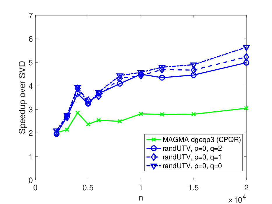
In summary, we present powerURV and randUTV for computing rank-revealing factorizations on a GPU. Both methods are much faster than the SVD. Compared to HQRCP, they are faster for sufficiently large matrices and much more accurate. As an example, Figure 1 shows the running time of the four methods on two Intel 18-core CPUs and an NVIDIA GPU.
Remark 1.
In this manuscript, we assume that the input and output matrices reside in CPU main memory in our numerical experiments, and reported compute times include the communication time for transferring data to and from the GPU. The storage complexity of all methods discussed is for an matrix. We restrict our attention to the case where all the data used in the computation fits in RAM on the GPU, which somewhat limits the size of matrices that can be handled. For instance, in the numerical experiments reported in Section 6, the largest problem size we could handle involved matrices of size about . The techniques can be modified to allow larger matrices to be handled and for multiple GPUs to be deployed, but we leave this extension for future work.
1.4. Outline of paper
In Section 2, we survey previous work in rank-revealing factorizations, discussing competing methods as well as previous work in randomized linear algebra that is foundational for the methods presented in this article. Section 3 presents the first algorithmic contribution of this article, powerURV. In Section 4, we discuss and build on the recently developed randUTV algorithm, culminating in a modification of the algorithm randUTV_boosted with greater potential for low rank estimation. Finally, Section 6 presents numerical experiments which demonstrate the computational efficiency of powerURV and randUTV_boosted as well as their effectiveness in low rank estimation.
2. Preliminaries
2.1. Basic notation
In this manuscript, we write to denote a real-valued matrix with rows and columns, and refers to the element in the -th row and -th column of . The indexing notation is used to reference the submatrix of consisting of the entries in the -th through -th rows of the -th through -th columns. is the -th singular value of , and is the transpose. The row and column spaces of are denoted as Row() and Col(), respectively. An orthonormal matrix is a matrix whose columns have unit norm and are pairwise orthogonal, and an orthogonal matrix is a square orthonormal matrix. The default norm is the spectral norm. If all the entires of a matrix are independent, identically distributed standard Gaussian variables, we call a standard Gaussian matrix, and we may denote it as . denotes the machine epsilon, say, in IEEE double precision
2.2. The singular value decomposition (SVD)
Given a matrix and , the (full) SVD of takes the form
where and are orthogonal, and is (rectangular) diagonal. The diagonal elements of are the singular values of and satisfy . The columns and of and are called the left and right singular vectors, respectively, of . In this article, we write for computing the (full) SVD decomposition of . Importantly, the SVD provides theoretically optimal rank- approximations to . Specifically, the Eckart-Young-Mirsky Theorem [22, 41] states that given the SVD of a matrix and a fixed , we have that
and the relation also holds with respect to the Frobenius norm.
The thin SVD of takes the form
where and are orthonormal, and is diagonal containing the singular values.
2.3. The column pivoted QR (CPQR) decomposition
Given a matrix , the (full) CPQR decomposition of takes the form
where is orthogonal, is trapezoidal, and is a permutation matrix. There exists a number of algorithms for choosing the permutation, but a general option, as implemented in LAPACK99 9 https://www.netlib.org/lapack/lug/node42.html, ensures monotonic decay in magnitude of the diagonal entries of so that . The details of the most popular algorithm for computing such a factorization, called HQRCP hereafter, are not essential to this article, but they may be explored by the reader in, e.g. [10, 27, 54, 49]. In this article, we write for computing the CPQR decomposition of .
It is well known that HQRCP is not guaranteed to be rank-revealing, and it can fail by an exponentially large factor (on, e.g. Kahan matrices) [31]. Such pathological cases are rare, particularly in practice, and HQRCP is so much faster than computing an SVD that HQRCP is used ubiquitously for low rank approximation. A communication avoiding variant based on “tournament pivoting” is given in [18], with a related method for fully pivoted LU described in [29].
2.4. The unpivoted QR decomposition
Given a matrix , the full (unpivoted) QR decomposition of takes the form
where is orthogonal, and is trapezoidal. When , the thin (unpivoted) QR decomposition of takes the form
where is orthonormal, and is upper triangular. Unpivoted QR decompositions have no rank-revealing properties, but in this article we make critical use of the fact that if and has full column rank, then the columns of form an orthonormal basis for Col().
The standard algorithm for computing an unpivoted QR factorization relies on Householder reflectors. We shall call this algorithm as HQR in this article and write or . We refer the reader once again to textbooks such as [27, 54, 49] for a complete discussion of the algorithm. The lack of the pivoting also allows HQR to rely more heavily on the level-3 BLAS than HQRCP, translating to better performance in parallel environments.
Of particular interest is the fact that the output orthogonal matrix of the HQR_full algorithm can be stored and applied efficiently even when . In HQR_full, suppose that we have determined Householder matrices such that We have that where is the Householder vector associated with the transformation. Then the matrix can be represented as
where is upper triangular and is lower trapezoidal with columns containing the [47]. The form of is called the compact-WY representation of a product of Householder reflectors.
Remark 2.
Observe that the compact-WY form reduces the storage requirement of from to and that the HQR_full algorithm requires work. More importantly, this representation of allows an efficient application of using matrix-matrix multiplications, which is crucial for efficiently building factorizations on a GPU.
If matrix is rank-deficient, i.e., , but the first columns in are linearly independent, then the HQR algorithm will detect this situation as and in exact arithmetic.
2.5. The randomized range finder
Consider a matrix and a block size such that . The randomized range finder algorithm [32] computes a set of orthonormal vectors that approximately span Row() or Col(). To be precise, suppose we seek to find an orthonormal matrix that
| (2) |
In other words, the columns of approximately span the same space as the dominant right singular vectors of . This task can be accomplished using randomized projections. An extremely simple way of building is the following:
- (1)
Generate a standard Gaussian matrix .
- (2)
Compute a “sampling matrix” .
- (3)
This method will yield a reasonably good approximation when the singular values of decay fast (see theoretical error bounds in, e.g. [32, Section 10]). However, for certain matrices, particularly when the decay in singular values is slow, an improved approximation will be desired. We may improve the approximation provided by in two ways:
- (1)
Oversampling: We may interpret as different random projections onto Row(). As shown in [32], the approximation of Col() to Row() may be improved by gathering a few, say , extra projections. In practice or is sufficient, adding very little additional computational cost ( extra work) to the algorithm. Using a small amount of oversampling also improves the expected error bounds and vastly decreases the probability of deviating from those bounds. For example, assume and while , it holds that [32, Corollary 10.9]
with failure probability at most , where are the singular values of . Thus, this technique makes the uses of randomization in the algorithm safe and reliable.
- (2)
Power iteration: In the construction of , we may replace the matrix with for , a matrix with the same column space as but whose singular values are . The contributions of singular vectors that correspond to smaller singular values will be diminished using this new matrix, thus improving the approximation of Col() to the desired singular vector subspace. 1111 11 See [46] for bounds on principle angles between the two subspaces. Again, assume and while , it holds that [32, Corollary 10.10]
where the constant depends on , , and . In other words, the power scheme drives the extra constant factor to one exponentially fast. In practice, the above error bound can be too pessimistic, and choosing to be , or gives excellent results. When using a power iteration scheme, numerical linear dependence of the samples becomes a concern since the information will be lost from singular vectors corresponding to singular values less than . To stabilize the algorithm, we build incrementally, orthonormalizing the columns of the intermediate matrix in between applications of and .
3. The powerURV algorithm.
Let be a given matrix. Without loss of generality, we assume ; otherwise, we may operate on instead. The powerURV algorithm is a slight variation of a randomized algorithm proposed by Demmel et al. [16] for computing a rank-revealing URV factorization of . The modification we propose makes the method more accurate in revealing the numerical rank, at only a marginal increase in computational time in a GPU environment. In addition, powerURV is remarkably simple to implement and has a close connection to the randomized SVD (RSVD) [32].
3.1. A randomized algorithm for computing a UTV factorization proposed by Demmel, Dumitriu, and Holtz
In [16], Demmel et al. give a randomized algorithm RURV (randomized URV) for computing a rank-revealing factorization of matrix . The algorithm can be written quite simply as follows:
- (1)
Generate a standard Gaussian matrix .
- (2)
- (3)
Compute .
- (4)
Note that after step (4), we have
a URV decomposition of (See [16, Sec. 5] for its rank-revealing properties.) A key advantage of this algorithm is its simplicity. Since it relies only on unpivoted QR and matrix multiplication computations, it can easily be shown to be stable (see [16] for the proof). Furthermore, both of these operations are relatively well-suited for parallel computing environments like GPUs. Since they are extremely common building blocks for problems involving matrices, highly optimized implementations for both are readily available. Thus, a highly effective implementation of RURV may be quickly assembled by a non-expert.
Demmel et al. find a use for RURV as a fundamental component of a fast, stable solution to the eigenvalue problem. For this application, RURV is used iteratively, so not much is required of the accuracy of the rank-revealing aspect of the resulting factorization. For other problems such as low-rank approximations, though, the error in (1) can be quite large (compared to, e.g., the powerURV algorithm that we are going to introduce; for interested readers, see [28, Figure 3] for a comparison of errors between RURV and powerURV). This is because the matrix does not incorporate any information from the row space of the input .
3.2. powerURV: A randomized algorithm enhanced by power iterations
The powerURV algorithm is inspired by the RURV of Section 3.1 combined with the observation that the optimal matrix to use for rank-revealing purposes (minimizing the error in (1)) is the matrix whose columns are the right singular vectors of the input matrix . If such a were used, then the columns of would be the left singular vectors of scaled by its singular values. Thus finding the right singular vectors of yields theoretically optimal low rank approximations. This subproblem is as difficult as computing the SVD of , though, so we settle for choosing as an efficiently computed approximation to the right singular vectors of
Specifically, we compute an approximation to the row space of using a variant of the randomized range finder algorithm in Section 2.5. The computation of consists of three steps:
- (1)
Generate a standard Gaussian matrix .
- (2)
Compute a “sampling matrix” , where is a small positive integer.
- (3)
The matrix can be thought of as a random projection onto the row space of . Specifically, the columns of are random linear combinations of the columns of . The larger the value of , the faster the singular values of the sampled matrix decay. Therefore, choosing to be large makes better aligned with the right singular vectors. It also increases the number of matrix multiplications required, but they execute efficiently on a GPU.
Unfortunately, a naive evaluation of is sensitive to the effects of roundoff errors. In particular, the columns of will lose the information provided by singular vectors with corresponding singular values smaller than . This problem can be remedied by orthonormalizing the columns of the intermediate matrices in between each application of and , employing extra unpivoted QR factorizations. The complete instruction set for powerURV is given in Algorithm 1.
3.3. Relationship with RSVD
The powerURV algorithm is closely connected to the standard randomized singular value decomposition algorithm (RSVD). The equivalency between RSVD and powerURV allows for much of the theory for analyzing the RSVD in [32, 46] to directly apply to the powerURV algorithm.
Let with and be a standard Gaussian matrix. Let , where is a positive integer. Let be a non-negative integer.
powerURV
Recall that powerURV has two steps. First, compute the full (unpivoted) QR factorization of :
| (3) |
where is orthogonal and is upper triangular. Second, compute the full (unpivoted) QR factorization of :
| (4) |
where is orthogonal and is upper trapezoidal.
RSVD
The RSVD builds an approximation to a truncated SVD via the following steps. First, evaluate
| (5) |
The columns of are orthonormalized via a thin (unpivoted) QR factorization1515 15 It is easy to show that , so has full rank with probability 1 according to Theorem 3 in Appendix A.
| (6) |
where is orthonormal, and is upper triangular and invertible. Next, the thin SVD of is computed to obtain
| (7) |
where is orthogonal, is orthonormal and is diagonal with singular values. We know all the singular values are positive because the columns of lie in Col. The final step is to define the matrix
| (8) |
The end result is an approximate SVD:
The key claim in this section is the following theorem:
Theorem 1.
Given two matrices , , and two integers , , as described at the beginning of Section 3.3, it holds that
where the two matrices and are computed by the powerURV and the RSVD, respectively, in exact arithmetic.
Proof.
We will prove that , which immediately implies that the two projectors and are identical. Let us first observe that restricting (3) to the first columns, we obtain
| (9) |
We can then connect and via a simple computation
| (10) | ||||
Next we link and via
| (11) |
Combining (10) and (11), we find that
| (12) |
We know that, with probability 1, matrices and are invertible, which establishes that . ∎
It is important to note that while there is a close connection between RSVD and powerURV, the RSVD is able to attain substantially higher overall accuracy than powerURV. Notice that the RSVD requires applications of either or , while powerURV requires only . The RSVD takes advantage of one additional application of in (7), where matrix rearranges the columns inside to make the leading columns much better aligned with the corresponding singular vectors. Another perspective to see it is that the columns of end up being a far more accurate basis for Row() than the columns of the matrix resulting from the powerURV. This is of course expected since for , the matrix incorporates no information from at all.
Remark 3.
Theorem 1 extends to the case when . The same proof will apply for a modified , and it is easy to see that adding additional columns to the basis matrices will make no difference since in this case .
Remark 4.
The RSVD requires an estimate of the numerical rank in order to compute a partial factorization. By contrast, the other methods discussed in this paper, which include the SVD, the column-pivoted QR (CPQR), and the two new methods (powerURV and randUTV), compute full factorizations without any a priori information about the numerical rank.
4. The randUTV algorithm.
In this section, we describe the randUTV algorithm. Throughout this section, is the input matrix. Without loss of generality, we assume (if , we may operate on instead). A factorization
where and are orthogonal and is upper trapezoidal is called a UTV factorization. Note that the SVD and CPQR are technically two examples of UTV factorizations. In the literature, however, a decomposition is generally given the UTV designation only if that is its most specific label; we will continue this practice in the current article. Thus, it is implied that is upper trapezoidal but not diagonal, and is orthogonal but not a permutation. The flexibility of the factors of a UTV decomposition allow it to act as a compromise between the SVD and CPQR in that it is not too expensive to compute but can reveal rank quite well. A UTV factorization can also be updated and downdated easily; see [49, Ch. 5, Sec. 4] and [24, 43, 48] for details.
randUTV is a blocked algorithm for computing a rank-revealing UTV decomposition of a matrix. It is tailored to run particularly efficiently on parallel architectures due to the fact that the bulk of its flops are cast in terms of matrix-matrix multiplication. The block size is a user-defined parameter which in practice is usually a number such as or (multiples of the tile size used in libraries such as cuBLAS). In Section 4.1, we review the original randUTV algorithm in [38]. Then, Section 4.2 presents methods of modifying randUTV to enhance the rank-revealing properties of the resulting factorization. Finally, in Section 4.3 we combine these methods with a bootstrapping technique to derive an efficient algorithm on a GPU.
4.1. The randUTV algorithm for computing a UTV decomposition
The algorithm performs the bulk of its work in a loop that executes iterations. We start with . In the -th iteration (), a matrix is formed by the computation
| (13) |
where and are orthogonal matrices chosen to ensure that satisfies the sparsity (nonzero pattern) and rank-revealing properties of the final factorization. Consider the first steps. Similar to other blocked factorization algorithms, the -th step is meant to “process” a set of columns of , so that after step , satisfies the following sparsity requirements:
- •
is upper trapezoidal, and
- •
the blocks on the main diagonal of are themselves diagonal.
After iterations, we compute the SVD of the bottom right block to obtain and . The sparsity pattern followed by the matrices is demonstrated in Figure 2.
 |
 | ||
| after 0 steps: | after 1 step: | after 2 steps: | after 3 steps: |
When the and matrices are desired, they can be built with the computations
In practice, the and are not stored separately to save memory. Instead, the space for , , and is allocated at the beginning of randUTV, and at iteration each is updated with
where and may be discarded or overwritten after an iteration completes.
To motivate the process of building and , consider the first step of randUTV. We begin by initializing and creating a helpful partition
where is , is , is , and is . The goal is to construct and such that, after the update ,
- (1)
is diagonal, (with entries that closely approximate the leading singular values of A)
- (2)
,
- (3)
,
- (4)
,
- (5)
.
Items (1) and (2) in the list are basic requirements for any UTV factorization, and the rest of the items relate to the decomposition’s rank-revealing properties.
The key observation is that if and were orthogonal matrices whose leading columns spanned the same subspace as the leading right and left singular vectors, respectively, of , items (2)-(4) in the previous list would be satisfied perfectly. (Items (1) and (5) could then be satisfied with an inexpensive post-processing step: compute the SVD of and update and accordingly.) However, determining the singular vector subspaces is as difficult as computing a partial SVD of . We therefore content ourselves with the goal of building and such that the spans of the leading columns are approximations of the subspaces spanned by the leading right and left singular vectors, respectively, of . We can achieve this goal efficiently using a variant of the randomized range finder algorithm discussed in Section 2.5. Specifically, we build as follows:
- (1)
Generate a standard Gaussian matrix .
- (2)
Sample Row() by calculating , where is a small non-negative integer.
- (3)
Once is built, the path to becomes clear after one observation. If the leading columns of span exactly the same subspace as the leading right singular vectors of , then the leading columns of span exactly the same subspace as the leading left singular vectors of . Therefore, after computing , we build as follows:
- (1)
Perform the matrix multiplication .
- (2)
Compute the full (unpivoted) QR factorization of to obtain an orthogonal matrix , i.e., . 1717 17 It is easy to show that, with probability 1, rank and the first columns in are linearly independent.
Following the same procedure, we can build and using the bottom right block for . At the last step, the SVD of the remaining block gives and . Then, we have
Notice that the transformation matrices and can be applied to the matrices efficiently as discussed in Section 2.4. We describe the basic randUTV algorithm, adapted from [40], in Appendix B.
An important feature of randUTV is that if a low-rank approximation of is needed, the factorization can be halted once a prescribed tolerance has been met. In particular, consider the following partition
where and contain the first columns in the corresponding matrices and is . The rank- approximation from randUTV is
and the approximation error is
| (14) |
where and are orthonormal matrices. Therefore, the factorization can be terminated as long as becomes smaller than a prescribed tolerance. In our blocked algorithm, we can calculate and check
at the -th iteration for .
For applications where errors are measured using the Frobenius norm, a more efficient algorithm is the following. Notice that (14) holds for the Frobenius norm as well. In fact, we have
where denotes the Frobenius norm. So we need to only pre-compute and update it with involving two small matrices at every iteration in randUTV. Specifically, we have
and
for . A similar approach for the RSVD was proposed in [56].
Remark 5.
The randUTV can be said to be a “blocked incremental RSVD” in the sense that the first step of the method is identical to the RSVD. In [38, Section 5.3], the authors demonstrate that the low-rank approximation error that results from the single-step randUTV factorization is identical to the error produced by the corresponding RSVD.
4.2. Using oversampling in the randUTV algorithm
In randUTV, the computation of matrix relies on the randomized range finder algorithm (discussed in Section 2.5). Just as the randomized range finder algorithm can use an oversampling parameter to improve the success probability, we add a similar parameter to the construction of in Algorithm 3 to improve the rank-revealing properties of the resulting factorization.
To do so, we first change the size of the random matrix from to (we once again consider only the building of to simplify matrix dimensions). This effectively increases the number of times we sample Row() by , providing a “correction” to the information in the first samples.
Next, we must modify how we obtain the orthonormal vectors that form . Recall that the first columns of must contain the approximation to the leading right singular vectors of . If we merely orthonormalized the columns of with HQR again, the first columns of would only contain information from the first columns of . We must therefore choose a method for building such that its first columns contain a good approximation of Col(). The following approaches use two of the most common rank-revealing factorizations to solve this subproblem:
- (1)
Perform a CPQR on to obtain the orthogonal matrix . The additional computational expense of computing HQRCP is relatively inexpensive for thin matrices like . However, the approximation provided by to Col() in this case will be suboptimal as mentioned in Section 2.3.
- (2)
Perform an SVD on to obtain an orthogonal matrix . Then contains the optimal rank- approximation of Col(). However, this method requires one more step since must be represented as a product of Householder vectors in order to compute efficiently in the following step of randUTV. After computing the SVD, therefore, we must perform a full (unpivoted) QR decomposition on , i.e., . 1818 18 We would have detected rank deficiency A with the SVD, and the first A columns in must be linearly independent. This method yields the optimal approximation of Col() given by .
In this article, we use method b) because it provides better approximations. As discussed in Remark 6 below, method b) requires a full (unpivoted) HQR of size , an SVD of size , and a full (unpivoted) HQR of size . While the SVD is small and therefore quite cheap, the first HQR is an extra expense which is nontrivial when aggregated across every iteration in randUTV. This extra cost is addressed and mitigated in Section 4.3.
Remark 6.
The SVD of method b) above may look expensive at first glance. However, recall that is of size , where . For tall, thin matrices like this, the SVD may be inexpensively computed as follows [9]:
- (1)
- (2)
Compute the SVD of the square matrix to obtain an orthogonal matrix with left singular vectors of , i.e., .
After these steps, we recognize that the matrix of left singular vectors of matrix is
The costs of the first step dominate the entire procedure, which are storage and work, respectively, according to Remark 2.
For randomized subspace iteration techniques like the one used to build the stability of the iteration is often a concern. As in the powerURV algorithm, the information from any singular values less than will be lost unless an orthonormalization procedure is used during intermediate steps of the computation . For randUTV, only singular vectors are in view in each iteration, so orthonormalization is not required as often as it is for powerURV.
However, if oversampling is used (), performing one orthonormalization before the final application of markedly benefits the approximation of Col() to the desired singular vector subspace. Numerical experiments show that this improvement occurs even when the sampling matrix is not in danger of loss of information from roundoff errors. Instead, we may intuitively consider that using orthonormal columns to sample ensures that the “extra” columns of contain information not already accounted for in the first columns.
4.3. Reducing the cost of oversampling and orthonormalization
Adding oversampling to randUTV, as discussed in Sections 4.2, adds noticeable cost to the algorithm. First, it requires a costlier method of building . Second, it increases the dimension of the random matrix , increasing the cost of all the operations involving and, therefore, . We will in this section demonstrate that the overhead caused by the latter cost can be essentially eliminated by recycling the “extra” information we collected in one step when we execute the next step.
To demonstrate, consider the state of randUTV for input matrix with after one step of the main iteration. Let denote the matrix for power iteration. At this point, we have computed and stored the following relevant matrices:
- •
: The matrix containing random samples of Row(), computed with
where is a standard Gaussian matrix.
- •
: The matrix whose columns are the left singular vectors of , computed with
see Section 4.2 method b).
- •
- •
- •
: The matrix being driven to upper trapezoidal form. At this stage in the algorithm,
Finally, consider the partitions
where and contain the first columns in corresponding matrices, and is .
In the second iteration of randUTV, the first step is to approximate Row(), where
Next, we make the observation that, just as Col() approximates the subspace spanned by the leading right singular vectors of , the span of the first columns of approximates the subspace spanned by the leading -th through -th right singular vectors of . Thus, Col is an approximation of Col. This multiplication involving two small matrix dimensions is much cheaper than carrying out the full power iteration process.
Putting it all together, on every iteration of randUTV after the first, we build the sampling matrix of columns in two stages. First, we build without oversampling or orthonormalization as in Section 4.1. Second, we build
by reusing the samples from the last iteration. The complete algorithm, adjusted to improve upon the low-rank estimation accuracies of the original randUTV, is given in Algorithm 2.
5. Implementation details
As mentioned earlier, powerURV (Algorithm 1) and randUTV (Algorithm 2) mainly consist of Level-3 BLAS routines such as matrix-matrix multiplication (gemm), which can execute extremely efficiently on modern computer architectures such as GPUs. Two essential features of GPUs from the algorithmic design perspective are the following: (1) The amount of parallelism available is massive. For example, an NVIDIA V100 GPU has 5120 CUDA cores. (2) The costs of data-movement against computation are orders of magnitude higher. As a result, Level-1 or Level-2 BLAS routines do not attain a significant portion of GPUs’ peak performance.
Our GPU implementation of the powerURV algorithm and randUTV algorithm uses a mix of routines from the cuBLAS library2020 20 https://docs.nvidia.com/cuda/cublas/index.html from NVIDIA and the MAGMA library [52, 53, 20]. The MAGMA library is a collection of next generation linear algebra routines with GPU acceleration. For the powerURV algorithm, we use the gemm routine from cuBLAS and routines related to (unpivoted) QR decomposition from MAGMA. For the randUTV algorithm, we mostly use MAGMA routines except for the gemm routine from cuBLAS to apply the Householder reflectors (see Section 2.4). These choices are mainly guided by empirical performance.
Our implementation consists of a sequence of GPU level-3 BLAS calls. The matrix is copied to the GPU at the start, and all computations (with one exception, see below) are done on the GPU with no communication back to main memory until the computation completes.
The exception is that the SVD subroutines in MAGMA do not support any GPU interface that takes an input matrix on the GPU. This is a known issue of the MAGMA library, and we follow the common workaround: copy the input matrix from GPU to CPU and then call a MAGMA SVD subroutine (MAGMA copies the matrix back to GPU and computes its SVD).
Fortunately, the extra cost of data transfer is negligible because the matrices whose SVDs are needed in Algorithm 2 are all very small (of dimensions at most ).
6. Numerical results
In this section, we present numerical experiments to demonstrate the performance of powerURV (Algorithm 1) and randUTV (Algorithm 2). In particular, we compare them to the SVD and the HQRCP in terms of speed and accuracy. Since the SVD is the most accurate method, we use it as the baseline to show the speedup and the accuracy of other methods. Results of the SVD were obtained using the MAGMA routine MAGMA_DGESDD,2121 21 The DGESDD algorithm uses a divide-and-conquer algorithm, which is different from the DGESVD algorithm based on QR iterations. The former is also known to be faster for large matrices; see https://www.netlib.org/lapack/lug/node71.html and Table 1 with CPU timings of both DGESVD and DGESDD in [38] where all orthogonal matrices are calculated. Results of the HQRCP were obtained using the MAGMA routine MAGMA_DGEQP3, where the orthogonal matrix was calculated.
All experiments were performed on an NVIDIA Tesla V100 graphics card with 32 GB of memory, which is connected to two Intel Xeon Gold 6254 18-core CPUs at 3.10GHz. Our code makes extensive use of the MAGMA (Version 2.5.4) library linked with the Intel MKL library (Version 20.0). It was compiled with the NVIDIA compiler NVCC (Version 11.3.58) on the Linux OS (5.4.0-72-generic.x86_64).
6.1. Computational speed
In this section, we investigate the speed of powerURV and randUTV on the GPU and compare them to highly optimized implementations of the SVD and the HQRCP for the GPU. In Figures 3, 4, and 5, every factorization is computed on a standard Gaussian matrix . All methods discussed here are “direct” methods, whose running time does not depend on the input matrix but its size. We compare the times (in seconds) of different algorithms/codes, where the input and output matrices exist on the CPU (time for moving data between CPU and GPU is included).
In each plot, we divide the given time by to make the asymptotic relationships between each experiment more clear, where . The MAGMA routine magma_dgesdd for computing the SVD run out of memory when . Raw timing results are given in Table 1 in Appendix C.




We observe in Figure 3 that powerURV with power iterations consistently outperforms HQRCP. powerURV with power iterations delivers similar performance with HQRCP for large matrices, but arrives at the asymptotic region much faster. As expected, the SVD is much slower than the other two methods.
We observe in Figure 4 that randutv without oversampling handily outperforms HQRCP. The cost of increasing the parameter is also quite small due to the high efficiency of matrix multiplication on the GPU.
We observe in Figure 5 that randutv with oversampling still outperforms HQRCP when . In addition, observe that the distance between the lines for and is less than the distance between the lines for and . This difference is representative of the savings gained with bootstrapping technique whereby extra samples from one iteration are carried over to the next iteration.
To summarize, our results show that the two newly proposed algorithms (powerURV and randutv) both achieved clear speedups over the SVD. They are also faster than HQRCP for sufficiently large matrices.
6.2. Approximation error
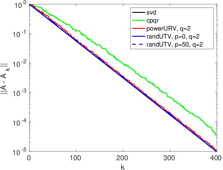
In this section, we compare the errors in the low-rank approximations produced by SVD, HQRCP, powerURV, and randUTV. Given an matrix , each rank-revealing factorization produces a decomposition
where and are orthogonal, and is upper triangular. Given this factorization, a natural rank- approximation to is
| (15) |
Recall in Section 2.2 that the rank- approximation produced by the SVD is the optimal among all rank- approximations, so we denote it as . For each of the factorizations that we study, we evaluated the error
| (16) |
as a function of , and report the results in Figures 6 and 7. Three different test matrices are considered:
- •
Fast decay: This matrix is generated by first creating random orthogonal matrices and by performing unpivoted QR factorizations on two random matrices with i.i.d entries drawn according to the standard normal distribution. Then, is computed with , where is a diagonal matrix with diagonal entries , where .
- •
S-shaped decay: This matrix is generated in the same manner as “fast decay,” but the diagonal entries are chosen to first hover around , then quickly decay before leveling out at , as shown in Figure 6(c).
- •
BIE: This matrix is the result of discretizing a boundary integral equation (BIE) defined on a smooth closed curve in the plane. To be precise, we discretized the so called “single layer” operator associated with the Laplace equation using a sixth order quadrature rule designed by Alpert [1]. This operator is well-known to be ill-conditioned, which necessitates the use of a rank-revealing factorization in order to solve the corresponding linear system in as stable a manner as possible.


Remark 7.
Remark 8.
As a curiosity, let us note that we have empirically observed that randUTV does surprisingly well at controlling relative errors. Figure 8 reports the error metric
for our three test matrices. We see that while CPQR does not manage to control this error, randUTV does a decent job, in particular when the power iteration is incorporated.
We make three observations based on results in Figures 6, 7, and 8. First, powerURV and randUTV are more accurate than HQRCP for a given . Errors from powerURV and randUTV are substantially smaller in almost all cases studied. Take Figure 6(a) as an example. The errors from HQRCP (green lines) are far from the minimals (black lines) achieved by SVD, whereas the errors from powerURV and randUTV (red and blue lines) are much closer to the minimals. It is also obvious in Figure 8 that the normalized errors from HQRCP (green lines) are usually larger (higher) than those from powerURV and randUTV (red and blue lines).
Second, randUTV is better than powerURV when the same steps of power iteration are used. For a large number of cases, errors from randUTV are significantly smaller. This is shown in Figure 6 that the blue lines (randUTV) lie in between the black lines (SVD) and the red lines (powerURV). It is more obvious in Figure 8 that the blue lines (randUTV) are lower than the red lines (powerURV).
Third, the new oversampling scheme in randUTV provides a boost in accuracies of low rank approximations obtained, even when the singular values decay slowly. The accuracy improvement is most pronounced when the singular values decay fast as shown in Figure 8(a). The figure also shows that without oversampling in randUTV, the accuracies of rank- approximations deteriorate when is approximately a multiple of the block size . This phenomenon is known in [32] and the reason of incorporating the oversampling scheme in randUTV.
7. Conclusions
The computation of a rank-revealing factorization has important applications in, e.g., low-rank approximation and subspace identification. While the SVD is theoretically optimal, computing the SVD of a matrix requires a significant amount of work that can not fully leverage modern parallel computing environments such as a GPU. For example, computing the SVD of an by matrix took more than a minute (79.4 seconds) on an NVIDIA V100 GPU.
We have described two randomized algorithms—powerURV and randUTV—as economical alternatives to the SVD. As we demonstrate through numerical experiments, both methods are much faster than the SVD on a GPU since they are designed to fully leverage parallel communication-constrained hardwares, and they provide close-to-optimal accuracy. The main features of the two new methods, respectively, include (1) powerURV has a simple formulation as shown in Algorithm 1 that it can be implemented easily on a GPU (or other parallel architectures), and (2) randUTV is a blocked incremental method that can be used to compute partial factorizations efficiently.
Compared to the CPQR factorization, which is commonly used as an economical alternative to the SVD for low-rank approximation, the new methods—powerURV and randUTV—are much more accurate and are similar or better in terms of speed on a GPU. Between the two methods, the randUTV is more accurate and generally faster, especially when power iteration is used. The accuracy of the randUTV can be further improved through the described oversampling technique (Section 4.2), which requires a modest amount of extra computation.
The two proposed methods can be viewed as evolutions of the RSVD. The distinction, however, is that the RSVD and related randomized methods for low-rank approximation [32, 36, 39]) work best when the numerical rank of an input matrix is much smaller than its dimensions. The key advantage of the two new methods is computational efficiency, in particular on GPUs, and they provide high speed for any rank.
Appendix A Results related to random matrices
Theorem 2.
Let be a standard Gaussian matrix. Then, with probability 1, has full rank.
Proof.
Without loss of generality, assume . It is obvious that
According to [45, Equation (3.2)], the probability that is singular equals zero. Therefore, the theorem holds. ∎
Theorem 3.
Let have rank and be a standard Gaussian matrix. Let . Then, with probability 1, matrix has rank and the first columns of are linearly independent.
Proof.
Let the thin SVD of be , where is an orthonormal matrix, is a diagonal matrix, and is an orthonormal matrix. Therefore,
Since also has the standard Gaussian distribution, it is full rank with probability 1 according to Theorem 2. So it is obvious that has full rank.
On the other hand, we know
Therefore, it holds that . ∎
Corollary 4.
Let have rank and be a standard Gaussian matrix. Let ( is invertible with probability 1 according to Theorem 2). Then, with probability 1, matrix has rank and the first columns of are linearly independent.
Proof.
Since , a unitary matrix, has full rank, we know .
Let . We know that
has full rank according to Theorem 3. So it is obvious that has full rank since is invertible with probability 1.
∎
Theorem 5.
Given a matrix , it holds that, for a positive integer ,
and, for a non-negative integer ,
Proof.
Suppose . Let the thin SVD of be , where and are orthonormal matrices, and is a diagonal matrix with the positive singular values. We know that
and
So it is obvious that the theorem holds. ∎
Appendix B randUTV algorithm adapted from [40].
Appendix C Raw data for Figure 3, 4, and 5
| SVD | HQRCP | powerURV | |||
|---|---|---|---|---|---|
| 3,000 | 1.98e+00 | 9.26e-01 | 5.06e-01 | 6.59e-01 | 9.38e-01 |
| 4,000 | 4.51e+00 | 1.58e+00 | 7.80e-01 | 9.79e-01 | 1.42e+00 |
| 5,000 | 5.97e+00 | 2.52e+00 | 1.13e+00 | 1.46e+00 | 1.92e+00 |
| 6,000 | 9.29e+00 | 3.66e+00 | 1.60e+00 | 2.14e+00 | 2.76e+00 |
| 8,000 | 1.85e+01 | 7.42e+00 | 2.68e+00 | 3.87e+00 | 5.29e+00 |
| 10,000 | 3.12e+01 | 1.11e+01 | 4.85e+00 | 7.29e+00 | 9.37e+00 |
| 12,000 | 4.74e+01 | 1.70e+01 | 7.62e+00 | 1.10e+01 | 1.50e+01 |
| 15,000 | 7.94e+01 | 2.84e+01 | 1.29e+01 | 1.94e+01 | 2.51e+01 |
| 20,000 | 1.71e+02 | 5.61e+01 | 2.85e+01 | 4.27e+01 | 6.03e+01 |
| 30,000 | N/A | 1.60e+02 | 9.12e+01 | 1.32e+02 | 1.87e+02 |
| randUTV () | randUTV () | |||||
|---|---|---|---|---|---|---|
| 3,000 | 7.20e-01 | 7.43e-01 | 7.34e-01 | 1.45e+00 | 1.72e+00 | 1.72e+00 |
| 4,000 | 1.14e+00 | 1.16e+00 | 1.23e+00 | 2.19e+00 | 2.56e+00 | 2.65e+00 |
| 5,000 | 1.83e+00 | 1.76e+00 | 1.84e+00 | 3.29e+00 | 3.72e+00 | 3.72e+00 |
| 6,000 | 2.49e+00 | 2.61e+00 | 2.53e+00 | 4.31e+00 | 4.95e+00 | 4.69e+00 |
| 8,000 | 4.17e+00 | 4.28e+00 | 4.52e+00 | 7.50e+00 | 7.93e+00 | 8.19e+00 |
| 10,000 | 6.82e+00 | 7.03e+00 | 6.94e+00 | 1.05e+01 | 1.22e+01 | 1.25e+01 |
| 12,000 | 9.89e+00 | 1.01e+01 | 1.09e+01 | 1.52e+01 | 1.72e+01 | 1.79e+01 |
| 15,000 | 1.62e+01 | 1.70e+01 | 1.78e+01 | 2.43e+01 | 2.73e+01 | 2.82e+01 |
| 20,000 | 3.03e+01 | 3.27e+01 | 3.43e+01 | 4.39e+01 | 5.10e+01 | 5.36e+01 |
| 30,000 | 9.25e+01 | 9.63e+01 | 1.04e+02 | 1.27e+02 | 1.50e+02 | 1.55e+02 |
References
- [1] Bradley K Alpert, Hybrid Gauss-trapezoidal quadrature rules, SIAM Journal on Scientific Computing 20 (1999), no. 5, 1551–1584.
- [2] Jesse L Barlow, Modification and maintenance of ULV decompositions, Applied Mathematics and Scientific Computing, Springer, 2002, pp. 31–62.
- [3] Mario Bebendorf and Sergej Rjasanow, Adaptive low-rank approximation of collocation matrices, Computing 70 (2003), no. 1, 1–24.
- [4] Christian H Bischof and Gautam M Shroff, On updating signal subspaces, IEEE Transactions on Signal Processing 40 (1992), no. 1, 96–105.
- [5] Ake Bjorck, Numerical methods for least squares problems, vol. 51, Siam, 1996.
- [6] L Susan Blackford, Antoine Petitet, Roldan Pozo, Karin Remington, R Clint Whaley, James Demmel, Jack Dongarra, Iain Duff, Sven Hammarling, Greg Henry, et al., An updated set of basic linear algebra subprograms (BLAS), ACM Transactions on Mathematical Software 28 (2002), no. 2, 135–151.
- [7] Andre R Brodtkorb, Christopher Dyken, Trond R Hagen, Jon M Hjelmervik, and Olaf O Storaasli, State-of-the-art in heterogeneous computing, Scientific Programming 18 (2010), no. 1, 1–33.
- [8] Peter Businger and Gene H Golub, Linear least squares solutions by Householder transformations, Numerische Mathematik 7 (1965), no. 3, 269–276.
- [9] Tony F Chan, An improved algorithm for computing the singular value decomposition, ACM Transactions on Mathematical Software (TOMS) 8 (1982), no. 1, 72–83.
- [10] by same author, Rank revealing QR factorizations, Linear algebra and its applications 88 (1987), 67–82.
- [11] Tony F Chan and Per Christian Hansen, Computing truncated singular value decomposition least squares solutions by rank revealing QR-factorizations, SIAM Journal on Scientific and Statistical Computing 11 (1990), no. 3, 519–530.
- [12] by same author, Some applications of the rank revealing QR factorization, SIAM Journal on Scientific and Statistical Computing 13 (1992), no. 3, 727–741.
- [13] Shivkumar Chandrasekaran and Ilse CF Ipsen, On rank-revealing factorisations, SIAM Journal on Matrix Analysis and Applications 15 (1994), no. 2, 592–622.
- [14] Kenneth L Clarkson and David P Woodruff, Low-rank approximation and regression in input sparsity time, Journal of the ACM (JACM) 63 (2017), no. 6, 54.
- [15] Jan JM Cuppen, A divide and conquer method for the symmetric tridiagonal eigenproblem, Numerische Mathematik 36 (1980), no. 2, 177–195.
- [16] James Demmel, Ioana Dumitriu, and Olga Holtz, Fast linear algebra is stable, Numerische Mathematik 108 (2007), no. 1, 59–91.
- [17] James W Demmel, Applied numerical linear algebra, SIAM, 1997.
- [18] James W Demmel, Laura Grigori, Ming Gu, and Hua Xiang, Communication avoiding rank revealing qr factorization with column pivoting, SIAM Journal on Matrix Analysis and Applications 36 (2015), no. 1, 55–89.
- [19] Yijun Dong and Per-Gunnar Martinsson, Simpler is better: a comparative study of randomized algorithms for computing the cur decomposition, arXiv preprint arXiv:2104.05877 (2021).
- [20] Jack Dongarra, Mark Gates, Azzam Haidar, Jakub Kurzak, Piotr Luszczek, Stanimire Tomov, and Ichitaro Yamazaki, Accelerating numerical dense linear algebra calculations with gpus, Numerical Computations with GPUs (2014), 1–26.
- [21] Petros Drineas, Ravi Kannan, and Michael W. Mahoney, Fast Monte Carlo algorithms for matrices. II. Computing a low-rank approximation to a matrix, SIAM J. Comput. 36 (2006), no. 1, 158–183 (electronic). MR MR2231644 (2008a:68243)
- [22] Carl Eckart and Gale Young, The approximation of one matrix by another of lower rank, Psychometrika 1 (1936), no. 3, 211–218.
- [23] Ricardo D. Fierro and Per Christian Hansen, Low-rank revealing UTV decompositions, Numerical Algorithms 15 (1997), no. 1, 37–55.
- [24] Ricardo D Fierro, Per Christian Hansen, and Peter Søren Kirk Hansen, UTV tools: Matlab templates for rank-revealing UTV decompositions, Numerical Algorithms 20 (1999), no. 2-3, 165.
- [25] Gene Golub, Numerical methods for solving linear least squares problems, Numerische Mathematik 7 (1965), no. 3, 206–216.
- [26] Gene H Golub and Charles F Van Loan, An analysis of the total least squares problem, SIAM journal on numerical analysis 17 (1980), no. 6, 883–893.
- [27] Gene H. Golub and Charles F. Van Loan, Matrix computations, third ed., Johns Hopkins Studies in the Mathematical Sciences, Johns Hopkins University Press, Baltimore, MD, 1996.
- [28] Abinand Gopal and Per-Gunnar Martinsson, The powerURV algorithm for computing rank-revealing full factorizations, arXiv preprint arXiv:1812.06007 (2018).
- [29] Laura Grigori, Sebastien Cayrols, and James W Demmel, Low rank approximation of a sparse matrix based on lu factorization with column and row tournament pivoting, SIAM Journal on Scientific Computing 40 (2018), no. 2, C181–C209.
- [30] Ming Gu and Stanley C Eisenstat, A divide-and-conquer algorithm for the bidiagonal SVD, SIAM Journal on Matrix Analysis and Applications 16 (1995), no. 1, 79–92.
- [31] by same author, Efficient algorithms for computing a strong rank-revealing qr factorization, SIAM Journal on Scientific Computing 17 (1996), no. 4, 848–869.
- [32] Nathan Halko, Per-Gunnar Martinsson, and Joel A. Tropp, Finding structure with randomness: Probabilistic algorithms for constructing approximate matrix decompositions, SIAM Review 53 (2011), no. 2, 217–288.
- [33] William Kahan, Numerical linear algebra, Canadian Mathematical Bulletin 9 (1966), no. 5, 757–801.
- [34] Ivars P Kirsteins and Donald W Tufts, Adaptive detection using low rank approximation to a data matrix, IEEE Transactions on Aerospace and Electronic Systems 30 (1994), no. 1, 55–67.
- [35] Charles L Lawson and Richard J Hanson, Solving least squares problems, vol. 15, Siam, 1995.
- [36] Edo Liberty, Franco Woolfe, Per-Gunnar Martinsson, Vladimir Rokhlin, and Mark Tygert, Randomized algorithms for the low-rank approximation of matrices, Proceedings of the National Academy of Sciences 104 (2007), no. 51, 20167–20172.
- [37] David Luebke, CUDA: Scalable parallel programming for high-performance scientific computing, 2008 5th IEEE international symposium on biomedical imaging: from nano to macro, IEEE, 2008, pp. 836–838.
- [38] Per-Gunnar Martinsson, Gregorio Quintana-Ortí, and Nathan Heavner, randUTV: A blocked randomized algorithm for computing a rank-revealing UTV factorization, ACM Transactions on Mathematical Software (TOMS) 45 (2019), no. 1, 1–26.
- [39] Per-Gunnar Martinsson, Vladimir Rokhlin, and Mark Tygert, A randomized algorithm for the decomposition of matrices, Applied and Computational Harmonic Analysis 30 (2011), no. 1, 47–68.
- [40] P.G. Martinsson and S. Voronin, A randomized blocked algorithm for efficiently computing rank-revealing factorizations of matrices, SIAM Journal on Scientific Computing 38 (2016), no. 5, S485–S507.
- [41] Leon Mirsky, Symmetric gauge functions and unitarily invariant norms, The quarterly journal of mathematics 11 (1960), no. 1, 50–59.
- [42] John D Owens, Mike Houston, David Luebke, Simon Green, John E Stone, and James C Phillips, GPU computing, (2008).
- [43] Haesun Park and Lars Eldén, Downdating the rank-revealing URV decomposition, SIAM Journal on Matrix Analysis and Applications 16 (1995), no. 1, 138–155.
- [44] Gregorio Quintana-Ortí, Xiaobai Sun, and Christian H. Bischof, A BLAS-3 version of the QR factorization with column pivoting, SIAM Journal on Scientific Computing 19 (1998), no. 5, 1486–1494.
- [45] Mark Rudelson and Roman Vershynin, Non-asymptotic theory of random matrices: extreme singular values, Proceedings of the International Congress of Mathematicians 2010 (ICM 2010) (In 4 Volumes) Vol. I: Plenary Lectures and Ceremonies Vols. II–IV: Invited Lectures, World Scientific, 2010, pp. 1576–1602.
- [46] Arvind K Saibaba, Randomized subspace iteration: Analysis of canonical angles and unitarily invariant norms, SIAM Journal on Matrix Analysis and Applications 40 (2019), no. 1, 23–48.
- [47] Robert Schreiber and Charles Van Loan, A storage-efficient WY representation for products of Householder transformations, SIAM Journal on Scientific and Statistical Computing 10 (1989), no. 1, 53–57.
- [48] Gilbert W Stewart, An updating algorithm for subspace tracking, IEEE Transactions on Signal Processing 40 (1992), no. 6, 1535–1541.
- [49] by same author, Matrix algorithms: Volume 1: Basic decompositions, vol. 1, Siam, 1998.
- [50] GW Stewart, Rank degeneracy, SIAM Journal on Scientific and Statistical Computing 5 (1984), no. 2, 403–413.
- [51] by same author, UTV decompositions, PITMAN RESEARCH NOTES IN MATHEMATICS SERIES (1994), 225–225.
- [52] Stanimire Tomov, Jack Dongarra, and Marc Baboulin, Towards dense linear algebra for hybrid GPU accelerated manycore systems, Parallel Computing 36 (2010), no. 5-6, 232–240.
- [53] Stanimire Tomov, Rajib Nath, Hatem Ltaief, and Jack Dongarra, Dense linear algebra solvers for multicore with GPU accelerators, Proc. of the IEEE IPDPS’10 (Atlanta, GA), IEEE Computer Society, April 19-23 2010, DOI: 10.1109/IPDPSW.2010.5470941, pp. 1–8.
- [54] Lloyd N Trefethen and David Bau III, Numerical linear algebra, vol. 50, Siam, 1997.
- [55] Field G Van Zee, Robert A Van de Geijn, and Gregorio Quintana-Ortí, Restructuring the tridiagonal and bidiagonal qr algorithms for performance, ACM Transactions on Mathematical Software (TOMS) 40 (2014), no. 3, 1–34.
- [56] Wenjian Yu, Yu Gu, and Yaohang Li, Efficient randomized algorithms for the fixed-precision low-rank matrix approximation, SIAM Journal on Matrix Analysis and Applications 39 (2018), no. 3, 1339–1359.