Two-Loop Four-Fermion Scattering Amplitude in QEDPreprint: MPP-2021-84; ZU-TH 29/21
Abstract
We present the first fully analytic evaluation of the transition amplitude for the scattering of a mass-less into a massive pair of fermions at the two-loop level in Quantum Electrodynamics. Our result is an essential ingredient for the determination of the electromagnetic coupling within scattering reactions, beyond the currently known accuracy, which has a crucial impact on the evaluation of the anomalous magnetic moment of the muon. It will allow, in particular, for a precise determination of the leading hadronic contribution to the in the MUonE experiment at CERN, and therefore can be used to shed light on the current discrepancy between the Standard Model prediction and the experimental measurement for this important physical observable.
Introduction – The Muon g-2 collaboration at Fermilab has recently confirmed Abi et al. 2021 that the observed magnetic activity of the muon is compatible with the earlier findings obtained at Brookhaven National Lab Bennett et al. 2002; Bennett et al. 2004; Bennett et al. 2006. The anomalous magnetic moment of the muon, , shows a deviation from the prediction of the Standard Model of elementary particles (SM) Aoyama et al. 2020. However, the theoretical determination of this quantity, obtained via dispersive techniques, might be affected by the improper estimation of the hadronic corrections to the muon–photon interaction, which could be responsible of such a discrepancy. Alternative results obtained through lattice QCD calculations point towards a possible mitigation of the tension between theory and experiments Borsanyi et al. 2021.
Recently, a novel experiment, MUonE, has been proposed at CERN, with the goal of measuring the running of the effective electromagnetic coupling at low momentum transfer in the space-like region Abbiendi et al. 2017. As proposed in Carloni Calame et al. 2015, this measurement would provide an independent determination of the leading hadronic contribution to the . Such a measurement relies on the precise determination of the angles of the outgoing particles emerging from the elastic muon-electron scattering Abbiendi et al. 2017; Abbiendi 2019; Abbiendi et al. 2020; Abbiendi et al. 2021. To extract the running of the effective electromagnetic coupling from the experimental data, the pure perturbative electromagnetic contribution to the electron-muon cross section must be controlled at least up to the second order in the fine-structure constant Banerjee et al. 2020a.
The scattering of a muon off an electron in Quantum Electrodynamics (QED) is the simplest reaction among fundamental leptons of different flavors, and represents a paradigmatic case of charged particles interaction mediated by a neutral gauge boson. The Leading Order (LO) process is known since the mid 1950’s Berestetskii and Pomeranchuk 1956, while the Next-to-Leading Order (NLO) radiative corrections were computed in Nikishov 1961; Eriksson 1961; Eriksson et al. 1963; Van Nieuwenhuizen 1971; Kukhto et al. 1987; Bardin and Kalinovskaya 1997; Kaiser 2010, and more recently studied in Alacevich et al. 2019. The two-loop diagrams contributing to the Next-to-Next-to-leading order (NNLO) virtual corrections were evaluated in Bern et al. 2001 assuming purely massless fermions. At the energies of the MUonE experiment, the muon mass plays an important role for the description of the radiative pattern and cannot be neglected Banerjee et al. 2020a. Nevertheless, the evaluation of Feynman integrals usually becomes more demanding as the number of massive particles present either in the loops or in the external states increases.
NNLO QED corrections involve the two-loop amplitude along with the real-virtual and the double-real emission terms. While the matrix elements for the last two contributions can be calculated without difficulties using standard techniques, their integration over the corresponding phase spaces is complicated by the presence of infrared (soft and collinear) singularities, as well as the presence of masses in both the initial and final state of the scattering process. In order to obtain predictions for fully differential observables, it is necessary to adopt a subtraction procedure. The Abelian nature of the interaction leads us to believe that the computational techniques already used for other processes at the LHC can be successfully adapted to this purpose Heinrich 2021; Torres Bobadilla et al. 2021. Preliminary Monte Carlo simulations for scattering have already been performed by including parts of the NNLO corrections Carloni Calame et al. 2020; Banerjee et al. 2020b. These simulations account for a subset of the two-loop graphs, not yet including the four-point diagrams with complete dependence on the lepton masses. The complete two-loop amplitude is then a missing crucial ingredient for the computation of the full NNLO QED corrections.
In this work, we present the first fully analytic evaluation of the renormalized two-loop amplitude for four fermion scattering in QED, , with and representing a massless and a massive lepton respectively. In the past years, we have developed efficient mathematical techniques for the evaluation of multi-loop integrals in dimensional regularization, such as the adaptive integrand decomposition Mastrolia et al. 2016a; Mastrolia et al. 2016b; Mastrolia et al. In preparation and the Magnus exponential method for differential equations Argeri et al. 2014; Di Vita et al. 2014. The combination of these techniques with the more traditional decomposition through integration-by-parts identities (IBPs) Chetyrkin and Tkachov 1981; Laporta 2000, allowed us to obtain for the first time a complete analytic formula for the renormalized two-loop amplitude of a process with a non-vanishing mass in internal and external lines.
The one- and two-loop amplitudes presented in this Letter can be applied, for instance, to the case where the light fermion is an electron, , and the heavy fermion is a muon, , and can be used in the elastic scattering , as well as in crossing related processes, such . If the elastic scattering is the key process of the MUonE experiment, the muon pair production in annihilation is a key process for the center-of-mass energy calibration at present and future colliders, such as BESIII Ablikim et al. 2017, BELLE-II Altmannshofer et al. 2019, CEPC Smiljanić et al. 2021, and FCCee Blondel et al. 2019. Therefore, a precise knowledge of the radiative effects would improve the precision of the results obtainable at these machines.
The structure of the infrared (IR) singularities of the massless and massive gauge theory scattering amplitudes has been studied in Catani 1998; Sterman and Tejeda-Yeomans 2003; Aybat et al. 2006a; Aybat et al. 2006b; Gardi and Magnea 2009a; Gardi and Magnea 2009b; Becher and Neubert 2009a; Becher and Neubert 2020; Becher and Neubert 2009b; Penin 2005; Penin 2006; Mitov and Moch 2007; Becher and Melnikov 2007; Bonciani et al. 2008a; Bonciani et al. 2008b; Becher and Neubert 2009c. In this work, the determination of the virtual NNLO corrections is complemented by the investigation of the IR singularities of scattering amplitudes in QED, which involve massive particles, and whose universal structure can be determined within Soft Collinear Effective Theory (SCET), along the lines of the method presented in Becher and Neubert 2009b; Becher and Neubert 2009c. The agreement of the residual IR poles coming from the direct diagrammatic calculus of the renormalized amplitude with the IR poles predicted within SCET is an important validation of the diagrammatic calculation. We explicitly verify this agreement in the case of process.
Additionally, let us observe that the two-loop diagrams considered here, also appear in the (color stripped) Abelian subset of graphs contributing to heavy-quark pair production in Quantum Chromodynamics (QCD) Czakon 2008; Bonciani et al. 2008c; Bonciani et al. 2009; Bärnreuther et al. 2014; Badger et al. 2021. The similarities of the analytic structure of the two-loop amplitude between in QCD and in QED, where and are treated as massless, is exploited to test the structure of the singularities coming from QED diagrams through a tuned comparison to the Abelian part of known results in QCD.
Recently, the evaluation of integrals coming from planar diagrams Fael and Passera 2019; Fael 2019; Heller 2021 indicates that the computation of four-fermion scattering
amplitudes at two loops in QED, by keeping full dependence on the masses of all the involved leptons, might become the subject of near-future investigation.
Scattering Amplitude –
We consider the four-fermion scattering process involving a mass-less and a massive lepton pair,
| (1) |
with and . The Mandelstam invariants, defined as and , satisfy the condition .
The four-point bare amplitude admits a perturbative expansion in the bare coupling constant , which, up to the inclusion of the second-order corrections, reads
| (2) |
where indicates the -loop bare amplitude, and is the ’t Hooft mass scale. The Leading Order (LO) term , referred to as Born term, receives contribution from a single tree-level Feynman diagram, shown in the upper row of Fig. 1. The squared LO amplitude, summed over the final spins and averaged over the initial states, reads,
| (3) |
for external states treated in space-time dimensions according to the conventional dimensional regularization (CDR) scheme Gnendiger et al. 2017, that we use throughout the whole computation. The interferences of one- and two-loop bare amplitudes with the Born amplitude read
| (4) |
Analytic Evaluation – The analytic evaluation of and is completely automated, within an in-house software, which can be applied to generic one- and two-loop amplitudes. The Mathematica package FeynArts Hahn 2001 is used to generate Feynman diagrams contributing to the one- and two-loop corrections to the scattering amplitudes as well as the counter-term diagrams required for the renormalization: 6 diagrams and 3 counter-term diagrams at one loop; 69 diagrams (12 of which vanish because of Furry’s theorem) and 55 counter-term diagrams at two loops. Representative one- and two-loop diagrams are shown in the second and third row of Fig. 1, respectively. The spin sums and the algebraic manipulation to simplify the Dirac- algebra are carried out by means of the FeynCalc Mertig et al. 1991; Shtabovenko et al. 2016; Shtabovenko et al. 2020 package. Each -loop graph (interfered with the Born amplitude) corresponds to an integrand written in terms of scalar products between external, , and internal, , momenta. Therefore, Eq.(4) can be generically written as,
| (5) |
where: indicates the numerator, and are the denominators corresponding to the internal lines of .
Integrands are simplified by employing the adaptive integrand decomposition method, implemented in the Aida framework Mastrolia et al. In preparation. The intermediate results emerging from the integrand decomposition can be further simplified by means of the IBP identities Chetyrkin and Tkachov 1981; Laporta 2000. Our software is interfaced with the publicly available codes Reduze von Manteuffel and Studerus 2012 and Kira Maierhfer et al. 2018, and, for each diagram, it produces the files for the automated generation of the IBP relations. After the decomposition phase, the interference terms are written as linear combination of a set of independent integrals, say , called master integrals (MIs),
| (6) |
where is a vector of coefficients, depending on and the kinematic variables, . In particular, and are conveniently expressed, in terms of 12 and 264 MIs, respectively, analytically computed: two- and three-point functions have been known since long Gehrmann and Remiddi 2000; Bonciani et al. 2003; Bonciani et al. 2004, while planar and non-planar four-point integrals were computed in Di Vita et al. 2018; Mastrolia et al. 2017, using the differential equation method via Magnus exponential, and independently in Bonciani et al. 2008c; Bonciani et al. 2009; Becchetti et al. 2019. The analytic expressions of can be written as a Laurent series around space-time dimensions (), with coefficients that contain Generalized Polylogarithms (GPLs) Goncharov 1998, defined as iterated integrals, through the recursive formula
| (7) |
with
.
The arguments are known as letters,
and their number, corresponding to the number of nested integrations, is called weight.
The two-loop interference term contains
4063 GPLs with up to weight four, whose arguments are written in terms of 18 letters, , which depend on the Mandelstam variables through the relations,
(see Di Vita et al. 2018; Mastrolia et al. 2017 for more details).
Renormalization – The one- and two-loop diagrams contributing to and contain infrared (IR) and ultraviolet (UV) divergences. To remove the UV divergences, the bare lepton fields (, with , for massless and massive leptons, respectively) and photon field (), as well as the bare mass of the massive lepton are renormalized as follows,
| (8) |
where, to simplify the notation, the label in the lepton fields is understood and restored when required. The renormalization of the QED interaction vertex,
| (9) |
can then be entirely fixed using the QED Ward identity, that implies . In particular, this leads to a simple relation between the renormalized charge and the bare charge (obtained by applying Eq. (8) to the bare interaction term and comparing the two renormalized expressions) , therefore, one has . The lepton wave functions and the mass of the massive lepton are renormalized in the on-shell scheme, namely, , , . The coupling constant is renormalized in the scheme at the scale ,
| (10) |
with . The renormalized amplitude is obtained by multiplying the bare amplitude with a factor for any external lepton , hence,
| (11) |
where , namely expressing the bare coupling and mass in terms of their renormalized counterparts. Let us observe that depends on four renormalization constants, namely . To simplify the notation in the following, these are simply indicated as , with , respectively. The renormalization constants admit a perturbative expansions in ,
| (12) |
and their expressions can be obtained (either directly or after abelianization) from Broadhurst et al. 1991; Melnikov and van Ritbergen 2000; Czakon et al. 2007; Bärnreuther et al. 2014. After substituting in Eq. (11) the expansions of the bare amplitude, given in Eq. (Two-Loop Four-Fermion Scattering Amplitude in QED), and the ones of the renormalization constants, given in Eq. (12), the UV renormalized two-loop amplitude reads
| (13) |
up to second order corrections in . The -loop coefficients are given in terms of the ones appearing in the bare amplitude as
| (14a) | |||||
| (14b) | |||||
| (14c) | |||||
The last term in Eq. (14c) contains the extra contribution of one-loop diagrams having an insertion of the mass counter-term in the massive propagators in all possible ways, as depicted in Fig. 2.
The bare coupling and the bare amplitudes
(),
appearing in Eqs. (42) and
(4),
can be replaced by the corresponding renormalized quantities
and
,
to build the Born term, ,
and the renormalized interference terms, at one loop,
, and at two loops, .
The latter two quantities constitute the
main results of this Letter.
Infrared Structure – The IR poles appearing in the two-loop corrections after UV renormalization can independently be obtained starting from the tree-level and the one-loop amplitudes, by following the same procedure employed to study the infrared structure of QCD amplitudes Becher and Neubert 2009b; Becher and Neubert 2009c.
The structure of the IR poles is governed by an anomalous dimension that has the following structure,
| (15) |
where the () coefficients up to are extracted in analogy to the QCD case Becher and Neubert 2009c; Becher and Neubert 2009b; Hill 2017. We compute the analytic expression of the two-loop amplitude for the process both in the non-physical region as well as directly in the production region. In this physical region, the imaginary part of the anomalous dimension in Eq. (Two-Loop Four-Fermion Scattering Amplitude in QED) is computed by adding an infinitesimal positive imaginary part to . One can then introduce the IR renormalization factor ,
| (16) |
where and are the coefficients of the expansion of , its derivative w.r.t. , and the QED beta function, respectively. The IR poles of the -order term can be calculated using and the lower order contributions, . In particular, the IR pole structures at one and two loops are found to be,
| (17a) | |||||
| (17b) | |||||
All functions in the r.h.s. of Eqs. (17) must be evaluated in space-time dimensions. The factors are the coefficients of the series expansion of in powers of .
The IR poles structure in Eqs. (17), reconstructed starting from the tree-level and one-loop amplitudes, is in perfect
agreement with the one obtained starting from Eq. (14c) and directly calculating the two-loop diagrams. This provides a non trivial test of the complete two-loop calculation.
Results – The analytic results of the interference contributions and are given as Laurent series in
| (18a) | |||||
| (18b) | |||||
The analytical expression of is computed both in the non-physical region, and in the pair production region, , . The latter is required to predict the IR poles of directly in the production region; the analytical expression of is computed in the non-physical region, , , and its analytic continuation is performed numerically. The renormalized one- and two-loop interference terms are conveniently decomposed in gauge-invariant components, labeled by the number of massless () and massive () closed fermion loops
| (19a) | |||||
| (19b) | |||||
In Fig. 3, we plot the finite part of one- and two-loop renormalized amplitudes , in the physical region. The threshold singularity is clearly visible and well reproduced up to
very small c.m.e., showing full control of the numerical stability.
The complete formula for the analytic expression of the renormalized two-loop amplitude is rather large (MB) and cannot be reported here. The figures are obtained by evaluating this formula with high precision on evenly spaced grid points,
by employing HandyG Naterop et al. 2020 and Ginac Vollinga and Weinzierl 2005 (via the package PolyLogtools Duhr and Dulat 2019) for the numerical evaluation of GPLs. Each evaluation required from seconds CPU time in the almost flat region to up about s CPU time for the configurations approaching the threshold singularity. These grids are available from the authors upon request.


Here, , .
Other tests – The master integrals for the Abelian diagrams in QED can be employed to construct the analytic expressions of some gauge-invariant contributions to the
two-loop amplitude of the process in QCD Czakon 2008; Bonciani
et al. 2008c; Bonciani et al. 2009; Bärnreuther et al. 2014: in particular, our results (evaluated in the region of heavy-lepton pair production, and properly accounting for the color factors) agree with the numerical coefficients provided in the Table 1 of Ref. Czakon 2008; Bonciani
et al. 2008c; Bärnreuther et al. 2014, which receive contributions from Abelian diagrams only;
the agreement on the poles of the above mentioned color coefficients, at
other phase-space points, has been verified using the formula for the IR poles of two-loop amplitudes in QCD, given in Ref. Ferroglia et al. 2009.
Conclusion – We presented the first fully analytic evaluation of the amplitude for the scattering of four fermions in Quantum Electrodynamics, involving two different types of leptons, one of which is treated as massless, up to the second order corrections in the electromagnetic coupling constant. The calculations were carried out within the dimensional regularization scheme, and the infrared pole structure of the renormalized amplitude is found to obey the universal behaviour predicted by the Soft Collinear Effective Theory. Our result constitutes the first example of a complete scattering amplitude for processes, with massless and massive particles in the loops as well as in the external states, involving planar and non-planar diagrams at two loops, analytically evaluated.
Our analytic results can be directly applied to the study, at NNLO accuracy, of massive lepton pair production in massless lepton annihilation, and, upon analytic continuation, to the study of the elastic scattering of massive and massless fermions in QED and QCD.
Notably, the virtual corrections presented here are relevant for the recently proposed
MUonE experiment at CERN.
This experiment is devoted to extraction of the hadronic contribution to the from
the scattering. The MUonE experiment analysis relies on the knowledge of the pure NNLO QED correction to the
scattering process, which will be the subject of a dedicated study in the near future.
Notes – Interested readers can find the expressions of the UV renormalization constants and of
the IR renormalization factor used throughout this Letter,
and additional plots for the individual contributions of the coefficients of Eq. (44) in the Supplemental Material.
Acknowledgments – We are indebted to Massimo Passera for insightful discussions, as well as for encouragement at all stages, and for comments on the manuscript. It is a pleasure to acknowledge the whole MUonE collaboration for motivating discussions, and for providing a stimulating scientific environment. In particular, we thank Matteo Fael and Massimo Passera for checks on the -corrections. We also thank Carlo Carloni Calame, Lance Dixon, Federico Gasparotto, Thomas Gehrmann, Stefano Laporta, Giovanni Ossola, Paride Paradisi, Fulvio Piccinini, Vajravelu Ravindran, Germán Rodrigo and Adrian Signer, for interesting discussions at various stages. The work of R.B. is partly supported by the italian Ministero della Università e della Ricerca (MIUR) under grant PRIN 20172LNEEZ. The work of A.B. is supported by the ERC Starting Grant REINVENT-714788. The work of A.F. is supported in part by the PSC-CUNY Award 62243-00 50. The work of M.K.M. is supported by Fellini - Fellowship for Innovation at INFN funded by the European Union’s Horizon 2020 research and innovation programme under the Marie Skłodowska-Curie grant agreement No 754496. The work of A.P. was supported by the Swiss National Science Foundation under grant number 200020-175595. J.R. and F.T. acknowledge support from INFN. U.S. is supported by the National Science Foundation awards PHY-1719690 and PHY-1652066. This work is supported by the COST Action CA16201 PARTICLEFACE.
I Supplemental Material
In this supplemental material, we provide further details on the renormalization constants to perform the UV renormalization, and the IR renormalization factor for the predictions of the IR poles of the one- and two-loop four-fermion scattering amplitude in QED, , with and , representing massless and a massive leptons, respectively.
Renormalization Constants –
The renormalization constants for the wave functions of the massive and massless leptons as well as the mass renormalization constant of the massive lepton admit perturbative expansions in , which can be taken
(either directly or after abelianization) from Refs. Broadhurst et al. 1991; Melnikov and van Ritbergen 2000; Czakon et al. 2007; Bärnreuther et al. 2014,
and read as,
| (20) | |||||
| (21) | |||||
| (22) |
where the individual perturbative coefficients in the on-shell scheme read as,
| (23) | |||||
| (24) | |||||
| (25) | |||||
| (26) |
with .
Additionally, the renormalization constant for the electromagnetic coupling up to second order in the scheme reads,
| (27) | |||||
Anomalous dimensions – The structure of the IR poles is governed by an anomalous dimension whose structure reads as,
| (28) |
and by the IR renormalization factor , defined by exponentiation of the following expression,
| (29) |
where and are the coefficient of the expansion of , its derivative w.r.t. , and the QED beta function, respectively. We hereby present the coefficients appearing in the above formulas, up to the needed order in :
| (30) |
The cusp anomalous dimensions for massless leptons have the coefficients Hill 2017,
| (31) |
whereas, for massive leptons,
| (32) | ||||
with defined through the relation,
| (33) |
The coefficients of the factors related to the massless and massive leptons are Hill 2017,
| (34) |
The QED beta function has the expansion
| (35) |
in which the only needed coefficient for the present calculation is ,
| (36) |
The quantity appearing in Eq. (I) is defined as,
| (37) |
with the relevant coefficients,
| (38) |
Furthermore, in order to implement the inverse decoupling transformation for the massive leptons, in such a way that one works with active leptons, one needs to include an additional term proportional to in :
| (41) |
where,


Here, , .

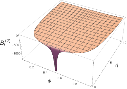


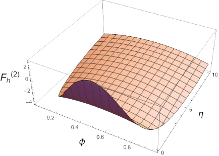
Here, , .
| - | - | - | - | |||
| - | - | |||||
| - | - | - | - | |||
| - | - | - | - | |||
| - | ||||||
| - | - | |||||
| - | - | - | ||||
| - | - | - | - | - | ||
| - | - | - | - | - | ||
| - | - | - | - | - |
Amplitudes – The Born term is shown in Eq.(3) of the Letter, reading as,
| (42) |
The results of the renormalized one- and the two-loop interference terms can be found in the Eqs.(15a,15b) of the Letter, as Laurent series in , hereby reported for conveninece,
| (43a) | |||||
| (43b) | |||||
Each term can be conveniently decomposed in gauge-invariant components, see Eqs.(16a,16b), as follows,
| (44a) | |||||
| (44b) | |||||
In Figs 1 and 2, we plot the finite parts of the individual form factors appearing in the decomposition of the one- and two-loop amplitudes, given in Eqs. (44). Finally, in Table 1, we showcase the numerical values of the coefficients in the massive-fermion pair production region at a particular phase-space point. Note that, upon accounting for a different definition of the Mandelstam variables, this benchmark point corresponds to the one used in Table 1 of Bärnreuther et al. 2014.
References
- Abi et al. (2021) B. Abi et al. (Muon g-2), Phys. Rev. Lett. 126, 141801 (2021), eprint 2104.03281.
- Bennett et al. (2002) G. W. Bennett et al. (Muon g-2), Phys. Rev. Lett. 89, 101804 (2002), [Erratum: Phys.Rev.Lett. 89, 129903 (2002)], eprint hep-ex/0208001.
- Bennett et al. (2004) G. W. Bennett et al. (Muon g-2), Phys. Rev. Lett. 92, 161802 (2004), eprint hep-ex/0401008.
- Bennett et al. (2006) G. W. Bennett et al. (Muon g-2), Phys. Rev. D 73, 072003 (2006), eprint hep-ex/0602035.
- Aoyama et al. (2020) T. Aoyama et al., Phys. Rept. 887, 1 (2020), eprint 2006.04822.
- Borsanyi et al. (2021) S. Borsanyi et al., Nature 593, 51 (2021), eprint 2002.12347.
- Abbiendi et al. (2017) G. Abbiendi et al., Eur. Phys. J. C77, 139 (2017), eprint 1609.08987.
- Carloni Calame et al. (2015) C. M. Carloni Calame, M. Passera, L. Trentadue, and G. Venanzoni, Phys. Lett. B746, 325 (2015), eprint 1504.02228.
- Abbiendi (2019) G. Abbiendi, Tech. Rep., CERN, Geneva (2019), URL https://cds.cern.ch/record/2677471.
- Abbiendi et al. (2020) G. Abbiendi et al., JINST 15, 01 (2020), eprint 1905.11677.
- Abbiendi et al. (2021) G. Abbiendi et al. (2021), eprint 2102.11111.
- Banerjee et al. (2020a) P. Banerjee et al., Eur. Phys. J. C 80, 591 (2020a), eprint 2004.13663.
- Berestetskii and Pomeranchuk (1956) V. Berestetskii and I. Pomeranchuk, JETP 2, 580 (1956).
- Nikishov (1961) A. Nikishov, JETP 12, 529 (1961).
- Eriksson (1961) K. E. Eriksson, Nuovo Cimento 19, 1029 (1961).
- Eriksson et al. (1963) K. E. Eriksson, B. Larsson, and G. A. Rinander, Nuovo Cimento 30, 1434 (1963).
- Van Nieuwenhuizen (1971) P. Van Nieuwenhuizen, Nucl. Phys. B28, 429 (1971).
- Kukhto et al. (1987) T. V. Kukhto, N. M. Shumeiko, and S. I. Timoshin, J. Phys. G13, 725 (1987).
- Bardin and Kalinovskaya (1997) D. Yu. Bardin and L. Kalinovskaya (1997), eprint hep-ph/9712310.
- Kaiser (2010) N. Kaiser, J. Phys. G37, 115005 (2010).
- Alacevich et al. (2019) M. Alacevich, C. M. Carloni Calame, M. Chiesa, G. Montagna, O. Nicrosini, and F. Piccinini, JHEP 02, 155 (2019), eprint 1811.06743.
- Bern et al. (2001) Z. Bern, L. J. Dixon, and A. Ghinculov, Phys. Rev. D 63, 053007 (2001), eprint hep-ph/0010075.
- Heinrich (2021) G. Heinrich, Phys. Rept. 922, 1 (2021), eprint 2009.00516.
- Torres Bobadilla et al. (2021) W. J. Torres Bobadilla et al., Eur. Phys. J. C 81, 250 (2021), eprint 2012.02567.
- Carloni Calame et al. (2020) C. M. Carloni Calame, M. Chiesa, S. M. Hasan, G. Montagna, O. Nicrosini, and F. Piccinini, JHEP 11, 028 (2020), eprint 2007.01586.
- Banerjee et al. (2020b) P. Banerjee, T. Engel, A. Signer, and Y. Ulrich, SciPost Phys. 9, 027 (2020b), eprint 2007.01654.
- Mastrolia et al. (2016a) P. Mastrolia, T. Peraro, and A. Primo, JHEP 08, 164 (2016a), eprint 1605.03157.
- Mastrolia et al. (2016b) P. Mastrolia, T. Peraro, A. Primo, and W. J. Torres Bobadilla, PoS LL2016, 007 (2016b), eprint 1607.05156.
- Mastrolia et al. (In preparation) P. Mastrolia, T. Peraro, A. Primo, J. Ronca, and W. J. Torres Bobadilla (In preparation).
- Argeri et al. (2014) M. Argeri, S. Di Vita, P. Mastrolia, E. Mirabella, J. Schlenk, U. Schubert, and L. Tancredi, JHEP 03, 082 (2014), eprint 1401.2979.
- Di Vita et al. (2014) S. Di Vita, P. Mastrolia, U. Schubert, and V. Yundin, JHEP 09, 148 (2014), eprint 1408.3107.
- Chetyrkin and Tkachov (1981) K. G. Chetyrkin and F. V. Tkachov, Nucl. Phys. B192, 159 (1981).
- Laporta (2000) S. Laporta, Int. J. Mod. Phys. A15, 5087 (2000), eprint hep-ph/0102033.
- Ablikim et al. (2017) M. Ablikim et al. (BESIII), Chin. Phys. C 41, 113001 (2017), eprint 1705.09722.
- Altmannshofer et al. (2019) W. Altmannshofer et al. (Belle-II), PTEP 2019, 123C01 (2019), [Erratum: PTEP 2020, 029201 (2020)], eprint 1808.10567.
- Smiljanić et al. (2021) I. Smiljanić, I. Božović-Jelisavčić, G. Kačarević, N. Vukašinović, T. Agatonović-Jovin, G. Milutinović-Dumbelović, J. Stevanović, and M. Radulović (CEPC), in International Workshop on Future Linear Colliders (2021), eprint 2105.06245.
- Blondel et al. (2019) A. Blondel et al. (2019), eprint 1909.12245.
- Catani (1998) S. Catani, Phys. Lett. B 427, 161 (1998), eprint hep-ph/9802439.
- Sterman and Tejeda-Yeomans (2003) G. F. Sterman and M. E. Tejeda-Yeomans, Phys. Lett. B 552, 48 (2003), eprint hep-ph/0210130.
- Aybat et al. (2006a) S. M. Aybat, L. J. Dixon, and G. F. Sterman, Phys. Rev. D 74, 074004 (2006a), eprint hep-ph/0607309.
- Aybat et al. (2006b) S. M. Aybat, L. J. Dixon, and G. F. Sterman, Phys. Rev. Lett. 97, 072001 (2006b), eprint hep-ph/0606254.
- Gardi and Magnea (2009a) E. Gardi and L. Magnea, JHEP 03, 079 (2009a), eprint 0901.1091.
- Gardi and Magnea (2009b) E. Gardi and L. Magnea, Nuovo Cim. C 32N5-6, 137 (2009b), eprint 0908.3273.
- Becher and Neubert (2009a) T. Becher and M. Neubert, Phys. Rev. Lett. 102, 162001 (2009a), [Erratum: Phys.Rev.Lett. 111, 199905 (2013)], eprint 0901.0722.
- Becher and Neubert (2020) T. Becher and M. Neubert, JHEP 01, 025 (2020), eprint 1908.11379.
- Becher and Neubert (2009b) T. Becher and M. Neubert, JHEP 06, 081 (2009b), [Erratum: JHEP 11, 024 (2013)], eprint 0903.1126.
- Penin (2005) A. A. Penin, Phys. Rev. Lett. 95, 010408 (2005), eprint hep-ph/0501120.
- Penin (2006) A. A. Penin, Nucl. Phys. B 734, 185 (2006), eprint hep-ph/0508127.
- Mitov and Moch (2007) A. Mitov and S. Moch, JHEP 05, 001 (2007), eprint hep-ph/0612149.
- Becher and Melnikov (2007) T. Becher and K. Melnikov, JHEP 06, 084 (2007), eprint 0704.3582.
- Bonciani et al. (2008a) R. Bonciani, A. Ferroglia, and A. A. Penin, Phys. Rev. Lett. 100, 131601 (2008a), eprint 0710.4775.
- Bonciani et al. (2008b) R. Bonciani, A. Ferroglia, and A. A. Penin, JHEP 02, 080 (2008b), eprint 0802.2215.
- Becher and Neubert (2009c) T. Becher and M. Neubert, Phys. Rev. D 79, 125004 (2009c), [Erratum: Phys.Rev.D 80, 109901 (2009)], eprint 0904.1021.
- Czakon (2008) M. Czakon, Phys. Lett. B 664, 307 (2008), eprint 0803.1400.
- Bonciani et al. (2008c) R. Bonciani, A. Ferroglia, T. Gehrmann, D. Maitre, and C. Studerus, JHEP 07, 129 (2008c), eprint 0806.2301.
- Bonciani et al. (2009) R. Bonciani, A. Ferroglia, T. Gehrmann, and C. Studerus, JHEP 08, 067 (2009), eprint 0906.3671.
- Bärnreuther et al. (2014) P. Bärnreuther, M. Czakon, and P. Fiedler, JHEP 02, 078 (2014), eprint 1312.6279.
- Badger et al. (2021) S. Badger, E. Chaubey, H. B. Hartanto, and R. Marzucca (2021), eprint 2102.13450.
- Fael and Passera (2019) M. Fael and M. Passera, Phys. Rev. Lett. 122, 192001 (2019), eprint 1901.03106.
- Fael (2019) M. Fael, JHEP 02, 027 (2019), eprint 1808.08233.
- Heller (2021) M. Heller (2021), eprint 2105.08046.
- Gnendiger et al. (2017) C. Gnendiger et al., Eur. Phys. J. C77, 471 (2017), eprint 1705.01827.
- Hahn (2001) T. Hahn, Comput. Phys. Commun. 140, 418 (2001), eprint hep-ph/0012260.
- Mertig et al. (1991) R. Mertig, M. Bohm, and A. Denner, Comput. Phys. Commun. 64, 345 (1991).
- Shtabovenko et al. (2016) V. Shtabovenko, R. Mertig, and F. Orellana, Comput. Phys. Commun. 207, 432 (2016), eprint 1601.01167.
- Shtabovenko et al. (2020) V. Shtabovenko, R. Mertig, and F. Orellana, Comput. Phys. Commun. 256, 107478 (2020), eprint 2001.04407.
- von Manteuffel and Studerus (2012) A. von Manteuffel and C. Studerus (2012), eprint 1201.4330.
- Maierhfer et al. (2018) P. Maierhfer, J. Usovitsch, and P. Uwer, Comput. Phys. Commun. 230, 99 (2018), eprint 1705.05610.
- Gehrmann and Remiddi (2000) T. Gehrmann and E. Remiddi, Nucl. Phys. B 580, 485 (2000), eprint hep-ph/9912329.
- Bonciani et al. (2003) R. Bonciani, P. Mastrolia, and E. Remiddi, Nucl. Phys. B 661, 289 (2003), [Erratum: Nucl.Phys.B 702, 359–363 (2004)], eprint hep-ph/0301170.
- Bonciani et al. (2004) R. Bonciani, P. Mastrolia, and E. Remiddi, Nucl. Phys. B 690, 138 (2004), eprint hep-ph/0311145.
- Di Vita et al. (2018) S. Di Vita, S. Laporta, P. Mastrolia, A. Primo, and U. Schubert, JHEP 09, 016 (2018), eprint 1806.08241.
- Mastrolia et al. (2017) P. Mastrolia, M. Passera, A. Primo, and U. Schubert, JHEP 11, 198 (2017), eprint 1709.07435.
- Becchetti et al. (2019) M. Becchetti, R. Bonciani, V. Casconi, A. Ferroglia, S. Lavacca, and A. von Manteuffel, JHEP 08, 071 (2019), eprint 1904.10834.
- Goncharov (1998) A. B. Goncharov, Math. Res. Lett. 5, 497 (1998), eprint 1105.2076.
- Broadhurst et al. (1991) D. J. Broadhurst, N. Gray, and K. Schilcher, Z. Phys. C 52, 111 (1991).
- Melnikov and van Ritbergen (2000) K. Melnikov and T. van Ritbergen, Nucl. Phys. B 591, 515 (2000), eprint hep-ph/0005131.
- Czakon et al. (2007) M. Czakon, A. Mitov, and S. Moch, Phys. Lett. B 651, 147 (2007), eprint 0705.1975.
- Hill (2017) R. J. Hill, Phys. Rev. D 95, 013001 (2017), eprint 1605.02613.
- Naterop et al. (2020) L. Naterop, A. Signer, and Y. Ulrich, Comput. Phys. Commun. 253, 107165 (2020), eprint 1909.01656.
- Vollinga and Weinzierl (2005) J. Vollinga and S. Weinzierl, Comput. Phys. Commun. 167, 177 (2005), eprint hep-ph/0410259.
- Duhr and Dulat (2019) C. Duhr and F. Dulat, JHEP 08, 135 (2019), eprint 1904.07279.
- Ferroglia et al. (2009) A. Ferroglia, M. Neubert, B. D. Pecjak, and L. L. Yang, JHEP 11, 062 (2009), eprint 0908.3676.